Article

Automated Negotiation Agents for Modeling Single-Peaked Bidders: An Experimental Comparison

by
Fatemeh Hassanvand
1,*,
Faria Nassiri-Mofakham
1,* and
Katsuhide Fujita
2,*
1
Faculty of Computer Engineering, University of Isfahan, Azadi Square, Isfahan 81746-73441, Iran
2
Institute of Global Innovation Research, Tokyo University of Agriculture and Technology, Tokyo 184-8588, Japan
*
Authors to whom correspondence should be addressed.
Information 2024, 15(8), 508; https://doi.org/10.3390/info15080508
Submission received: 23 July 2024 / Revised: 16 August 2024 / Accepted: 18 August 2024 / Published: 22 August 2024
(This article belongs to the Special Issue Intelligent Agent and Multi-Agent System)

Abstract

:
During automated negotiations, intelligent software agents act based on the preferences of their proprietors, interdicting direct preference exposure. The agent can be armed with a component of an opponent’s modeling features to reduce the uncertainty in the negotiation, but how negotiating agents with a single-peaked preference direct our attention has not been considered. Here, we first investigate the proper representation of single-peaked preferences and implementation of single-peaked agents within bidder agents using different instances of general single-peaked functions. We evaluate the modeling of single-peaked preferences and bidders in automated negotiating agents. Through experiments, we reveal that most of the opponent models can model our benchmark single-peaked agents with similar efficiencies. However, the accuracies differ among the models and in different rival batches. The perceptron-based P1 model obtained the highest accuracy, and the frequency-based model Randomdance outperformed the other competitors in most other performance measures.

1. Introduction

Negotiation, a seemingly mundane daily-life procedure, can turn numerous discords into accords. Negotiation is also the process by which devices and applications interact, cooperate, or compete for access to a particular resource in smart industries. For example, new generations of wireless networks (5G, 6G, and beyond) will enable the devices and applications in autonomous vehicles, autonomous industries, smart cities, and smart homes to interact with each other as independent entities. However, the tradeoff amongst the accuracy, delay, resource consumption, and other computational parameters must be properly balanced to deliver a high quality of service from each entity. This balance is akin to complex human negotiations, where multiple factors must be considered to reach a mutually beneficial agreement [1]. If the resources are limited, competition amongst these intelligent entities for a particular resource can engender severe discord and hinder all (or most) of the entities from accessing the resource. Automated negotiation, which has been extensively researched in multi-agent systems [2], coupled with distributed artificial intelligence could resolve such discord by allowing each party to authorize an autonomous agent to negotiate the resource exchange while retaining its preferences for single- or multi-issue alternatives that correspond with its owner’s preferences [3]. An agent can confront one rival (bilateral negotiation) or several rivals (multilateral negotiation).
Automated negotiation agents are useful for resolving conflicts in domains [4] such as task allocation [5], health care [6], urban planning [7], water resource management [8], and transportation [9] in which multiple stakeholders with different or opposing preferences must find a mutually acceptable solution.
The international Automated Negotiating Agents Competition (ANAC) [10] aims to establish efficient strategies and a common benchmark for negotiations. ANAC-participating agents are implemented in the bidding–opponent–acceptance (BOA) architecture [11], which comprises three components: (1) a bidding strategy that renders an offer when the agent’s turn approaches, (2) an opponent model that estimates the opponent’s trait(s), and (3) an acceptance strategy by which the agent accepts or rejects the opponent’s current offer. Unlike game theory [12], the preferences and utility spaces for possible alternatives are not common knowledge, and the agents negotiate with incomplete information. Consequently, to reach an effective agreement, every agent must create a model of its opponent’s preferences using exchanged offers. Such rarely known and gradually acquired partial information, along with an increasing volume of unlabeled data, encumber the learning preferences. Agents’ preferences over some issues are often single-peaked, meaning that the agent prefers a particular value over all other values. Estimating the peak point is essential for expediting the optimization of subsequent decisions. Despite the importance of arming the proper agents with preferences, cases with numerous agents with single-peaked preferences and whether the current agents can model single-peaked opponents have not been thoroughly investigated. We are aware of only two papers [13,14] focusing on the single-peaked preferences (e.g., [15]) of negotiating agents confronting single-peaked opponents. This paper advances the literature by exploring different representations of single-peaked preferences, including cardinal, ordinal, binary, and fuzzy structures. We delve into various utility functions, particularly the general triangular and skew normal distribution functions, to construct 18 distinct single-peaked preference profiles. By combining these utility functions with diverse time-dependent bidding strategies, we develop 162 single-peaked bidder agents. Furthermore, we conduct a comprehensive evaluation of the efficiency and accuracy of existing opponent models in capturing the behavior of these bidding agents. Our analysis identifies two perceptron-based opponent models [16] along with models extracted from ANAC’s agents during the 2010–2019 period as suitable for our research purposes. In addressing these contributions, the paper seeks to answer the following research questions:
  • What are the principal representations of single-peaked preferences across negotiation issues, and which representation is most suited to the context of automated negotiations?
  • How can single-peaked preferences be integrated into bidding agents?
  • How do current opponent models in negotiation agents accurately and efficiently model the behaviors of single-peaked bidding agents?
These questions aim to bridge the gap in the literature by providing a comprehensive analysis of single-peaked preferences within automated negotiations and their implications for agent design and opponent modeling.
Single-peaked preferences and opponent models are proposed as common benchmarks for agent strategy evaluations. Specifically, a single-peaked agent model is potentially more general and realistic than the popularly used weighted-sum and issue-based preference models. The remainder of this paper is structured as follows. Section 2 introduces bilateral multi-issue negotiation, and Section 3 discusses the concepts related to single-peaked preferences. Section 4 describes the research method and the construction of single-peaked agents. Section 5 describes the experiments and their evaluations. The results and key findings are discussed in Section 6, and Section 7 concludes the paper.

2. Bilateral Multi-Issue Negotiation

In automated negotiations, an issue is defined as a negotiable parameter with specific values to be reconciled by an agent. Issues range from contractual terms such as prices to logistical details such as delivery schedules. Each agent enters the negotiation with a set of preferences (ranked priorities or essential conditions) that it strives to achieve. These preferences are typically encoded in a utility function that assigns a numerical value to each potential outcome, aiding the attractiveness assessment of various proposals by the agent. The negotiation protocol outlines the structured process by which parties interact (including the offer exchange and decision-making processes) to ensure the orderly progression of the negotiation toward a potential agreement.

3. Single-Peaked Preferences

A preference structure represents the preferences of an agent from a set of alternatives that mainly appear as different features of a product or service. The four main structures of preference representations are outlined below [16]:
  • In the cardinal preference representation, the desirabilities of the alternatives are assigned within an outcome space X. The utility function is expressed as U : X Val , where Val is a set of quantitative or qualitative values.
  • In the ordinal preference representation, the alternatives share a binary relation ≼ (which is both reflexive and transitive).
  • In the binary preference representation, X is partitioned into a set of “good states” and “bad states”. This representation can be considered as a degenerate ordinal and cardinal preference structure.
  • In the fuzzy preference representation, a fuzzy relation in the form of ρ : X × X 0 , 1 where ρ x , y denotes the preference degree of x to y, is applied to X.
The present study utilizes a quantitative structure, which has been popularly applied as the preference representation in automated negotiations [17]. The utility function of a quantitative structure can be symmetric or asymmetric but must produce a single-peaked shape. In a symmetric utility function, the utility loss similarly deviates above and below the peak point [18], whereas asymmetric utility functions fall into one of two categories: shortfall avoidance (curve following the green squares in Figure 1) or excess avoidance (curve following the purple triangles in Figure 1). In shortfall avoidance, every alternative above the peak is preferred over its symmetric counterpart; that is, U e * d < U e * + d for all d, where d > 0 indicates the deviation from the peak, and U represents utility. Excess avoidance is characterized by the opposite behavior, with U e * d > U e * + d .
Representations of single-peaked preferences are generally expressed in the following three forms, each encompassing an inordinate number of single-peaked utility functions [18]:

3.1. Linex Loss Function

The Linex loss function, introduced by Varian [19], is commonly utilized in optimal forecasting [20] and in representations of policymakers’ preferences regarding output gaps and inflation [21]. The Linex loss function is formulated as
V ( x ) = exp α x * x + α x * x + 1 ,
where V x * = 0 , and α R . When α > 0 and α < 0 , the function represents shortfall and excess avoidance, respectively. Note that this function cannot represent every type of single-peaked preference.

3.2. Waud Function

The Waud function [22] is a piecewise function defined as
V ( x ) = λ f x * x x x * f x x * x > x *
where f is a strictly ascending and convex function with f ( 0 ) = 0 and λ > 0 . Here, λ < 1 and λ > 1 denote shortfall and excess avoidance, respectively. Like the Linex loss function, the Waud function cannot represent all types of single-peaked preferences.

3.3. Generalized Distance-Metric Utility Function

The generalized distance-metric utility function [18] is a distance-based representation of single-peaked preferences. It is defined as
V ( x ) = f x x * x 0 ,   x * f δ 1 x x * x x * , x ¯
where f denotes a continuous and strictly ascending distance function between the peak point x * and each desirable alternative x * . The distance function can be quadratic x x * 2 , the norm x x * , or any | x x * | λ for λ > 0 . To every deviation below the peak, the δ preference-bias function assigns the value above the peak for which the agent is indifferent. The reverse function δ 1 : R + R + determines the degree of asymmetry. Linear and nonlinear forms of δ 1 possess simple and intricate asymmetry, respectively.
In the present research, single-peaked preferences are represented and implemented using two instances of this general function.

4. Methodology

The present study assesses the accuracy and performance of modeling single-peaked preferences in bilateral multi-issue negotiations. To this end, we first create various single-peaked negotiating agents as benchmarks. Each benchmark single-peaked agent comprises two principal components: (1) a utility function that assigns a utility to each issue value and (2) a bidding strategy through which a negotiation proceeds. To generate a multitude of benchmark agents, we must combine various single-peaked utility functions with various bidding strategies. The configurations of the modeling and single-peaked agents are detailed below.

4.1. Single-Peaked Preference Profile

We first overview the single-peaked utility functions required for creating single-peaked agents.

4.1.1. Skew-Normal Distribution Function

This function can be symmetric or asymmetric [23] and is formulated as
f ( x , ω , p , α ) = 1 ω π e x p 2 2 ω 2 α x p ω e t 2 2 dt ,
where ω , p, and α denote the shape scale, peak point position, and skewness, respectively. The value of α determines whether the shape is symmetric or asymmetric, and an asymmetric shape can be right-skewed ( α > 0) or left-skewed ( α < 0). Unlike a previous paper that utilized symmetric shapes only [13], we utilize both symmetric and asymmetric forms of Equation (4). By varying the value of α as shown in Table 1, we generate six asymmetric shapes over a domain (cf. Section 5.2) with 1000 values (see Figure 2 for an example). Note that the values assigned to p are chosen such that the function generates the same shape in each desirable domain.

4.1.2. Gaussian Function

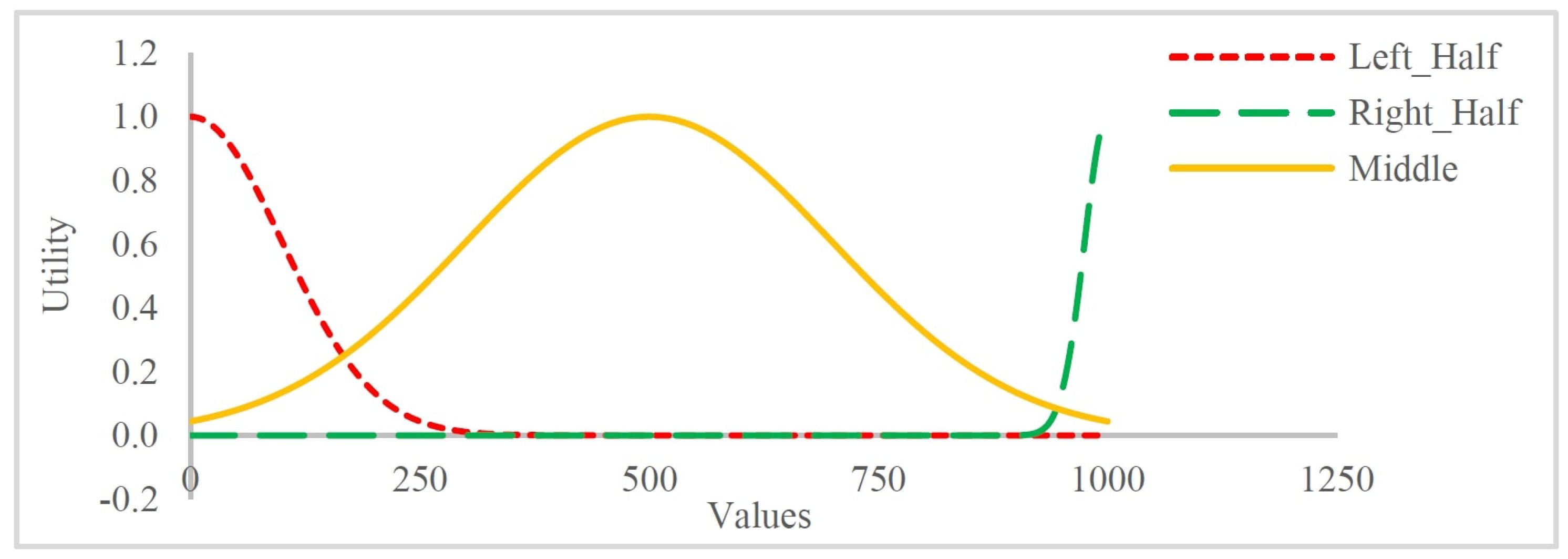
The Gaussian function is obtained by setting α = 0 in the skew-normal distribution given by Equation (4). This famous symmetric function is also called the normal distribution. Here, we utilize three symmetric shapes from a previous study [13] (see Table 2 for details and Figure 3 for a visual representation).

4.1.3. General Triangular Function

This function produces diverse symmetric and asymmetric shapes and is defined as
f ( x , L , R , p , λ , h ) = h 1 x p R p λ x < R h x L p L λ x < p 0 x < L
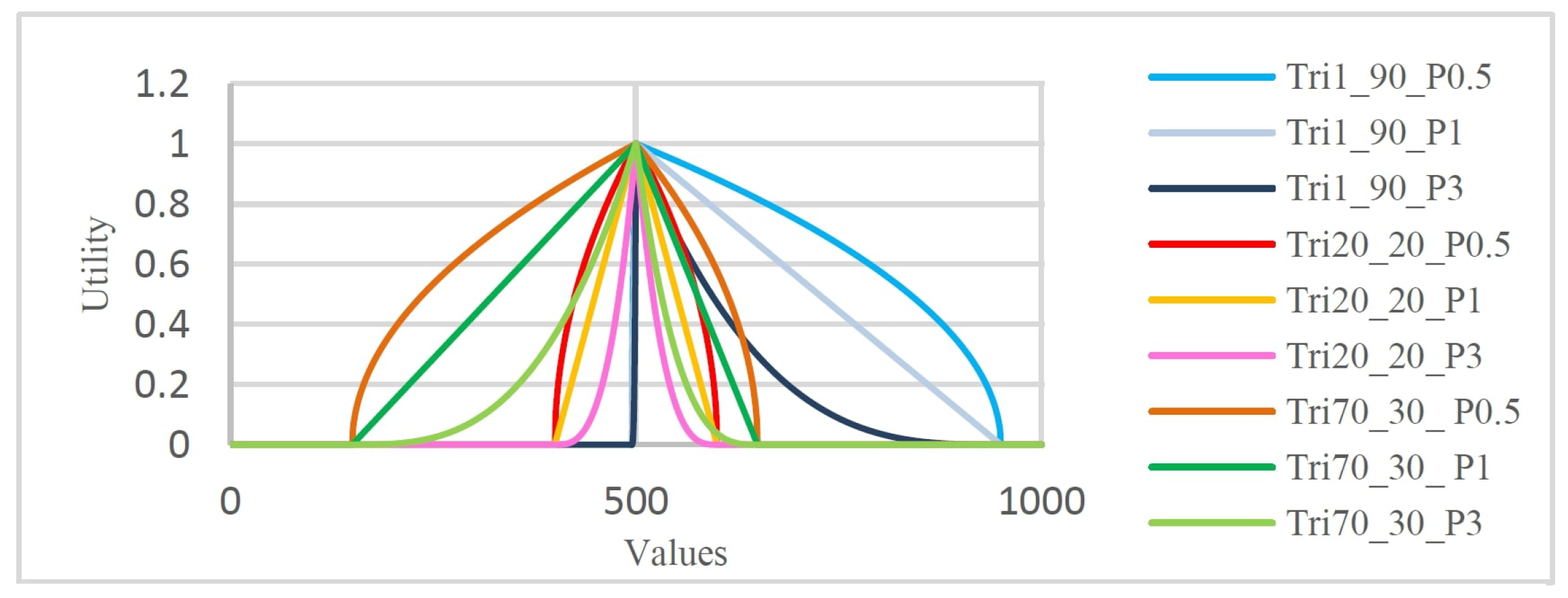
where L and R respectively denote the left and right minima (which meet the horizontal axis); p is a parameter that determines the peak position, and h is the height of the shape. The shape is symmetric if | p L | = | R p | , and it is asymmetric otherwise. With an extra parameter that determines the tightness of the peak’s shape, the general triangular function generates more diverse shapes than the previous two functions. More specifically, setting λ > 1 , λ = 1 , and 0 < λ < 1 will generate a narrow-peaked triangle, a standard triangle, and an embowed-peak triangle, respectively. In the present research, three symmetric and six asymmetric shapes were generated from the general triangular function. The chosen parameters are listed in Table 3, and their created shapes are plotted in Figure 4. For all shapes, we set h = 1 because the permittable utility range is [ 0 ,   1 ] ; that is, if the utility of one negotiation value exceeds 1, then all respective issue values must be normalized within [ 0 ,   1 ] . In addition, to avoid the scalability concerns of attaining similar shapes in all domains, we vary the percentages of L and R as shown in each column of Table 3. Consequently, we must calculate the exact position on the horizontal axis of Figure 4.

4.2. Constructing Single-Peaked Preference Profiles

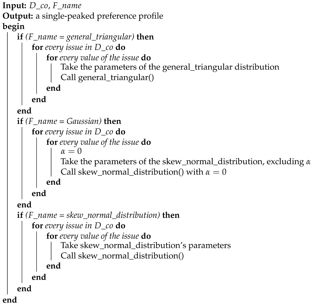
Single-peaked preference profiles are constructed by Algorithm 1. A copy of the negotiation domain is available to each negotiating agent. By invoking one of the single-peaked functions (cf. Section 4.1), a supposedly single-peaked agent creates its specific preference profile. For this purpose, the algorithm receives a copy of the domain plus the name of a single-peaked function: (1) general triangular, (2) Gaussian, or (3) skew-normal distribution. Proper parameter values of the selected single-peaked function must be passed for every negotiation issue. In other words, the chosen single-peaked function is applied to each issue in sequence. The algorithm executes lines 2–9 for calls to the general triangular distribution, lines 10–18 for calls to the Gaussian distribution, and lines 19–26 for calls to the skew-normal distribution. The pseudocodes of these functions are given in Algorithms 2 and 3. After passing these steps, the agent is ready to be armed with other components, such as a bidding strategy, acceptance strategy, and an opponent model, when required.
Algorithm 1 Creation of the single-peaked preference profile.
// The symbols: cf. Table 4
Information 15 00508 i001
Algorithm 2 General triangular function.
// The symbols, see Table 4
Information 15 00508 i002
Algorithm 3 Skew-normal distribution function.
// The symbols, cf. Table 4
Information 15 00508 i003

4.3. Configuration of the Single-Peaked Bidder Agent

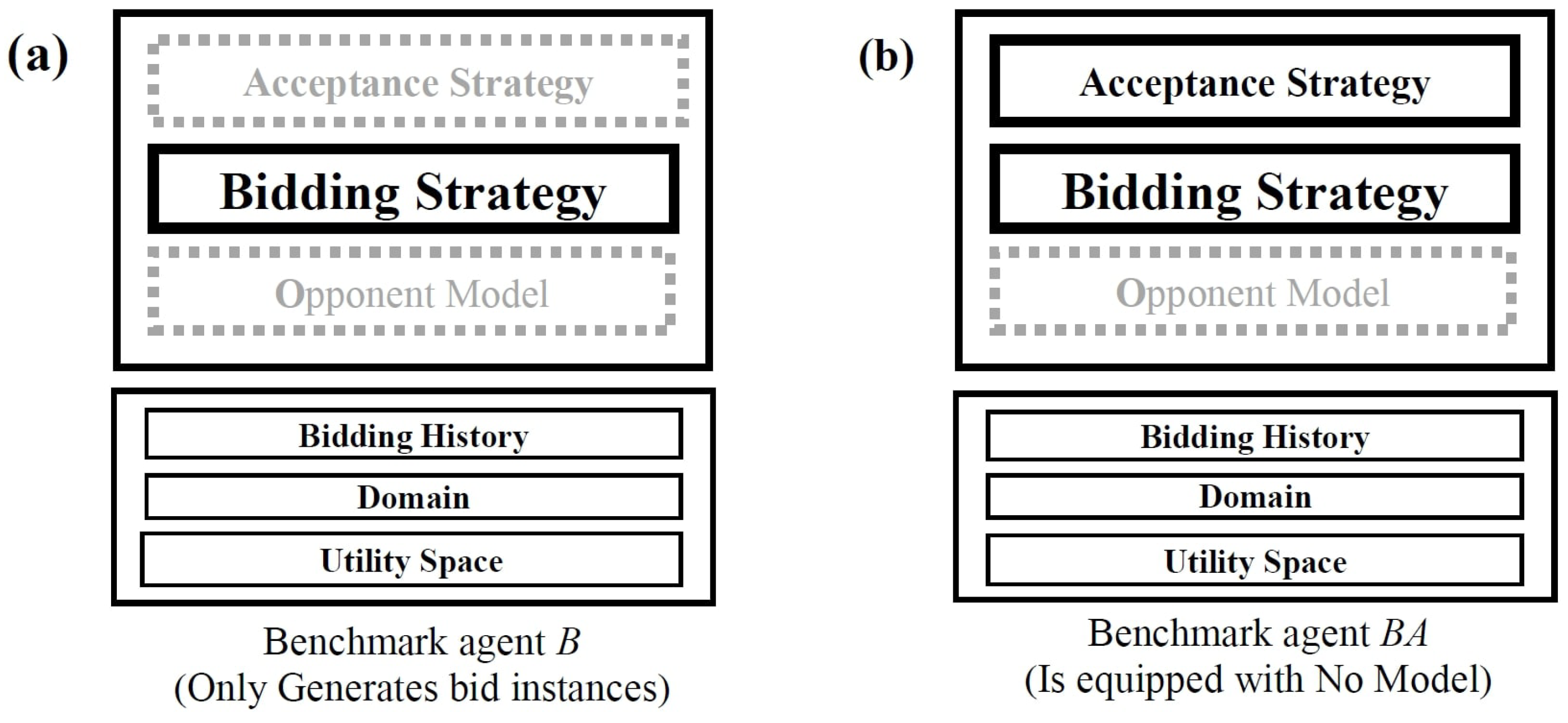
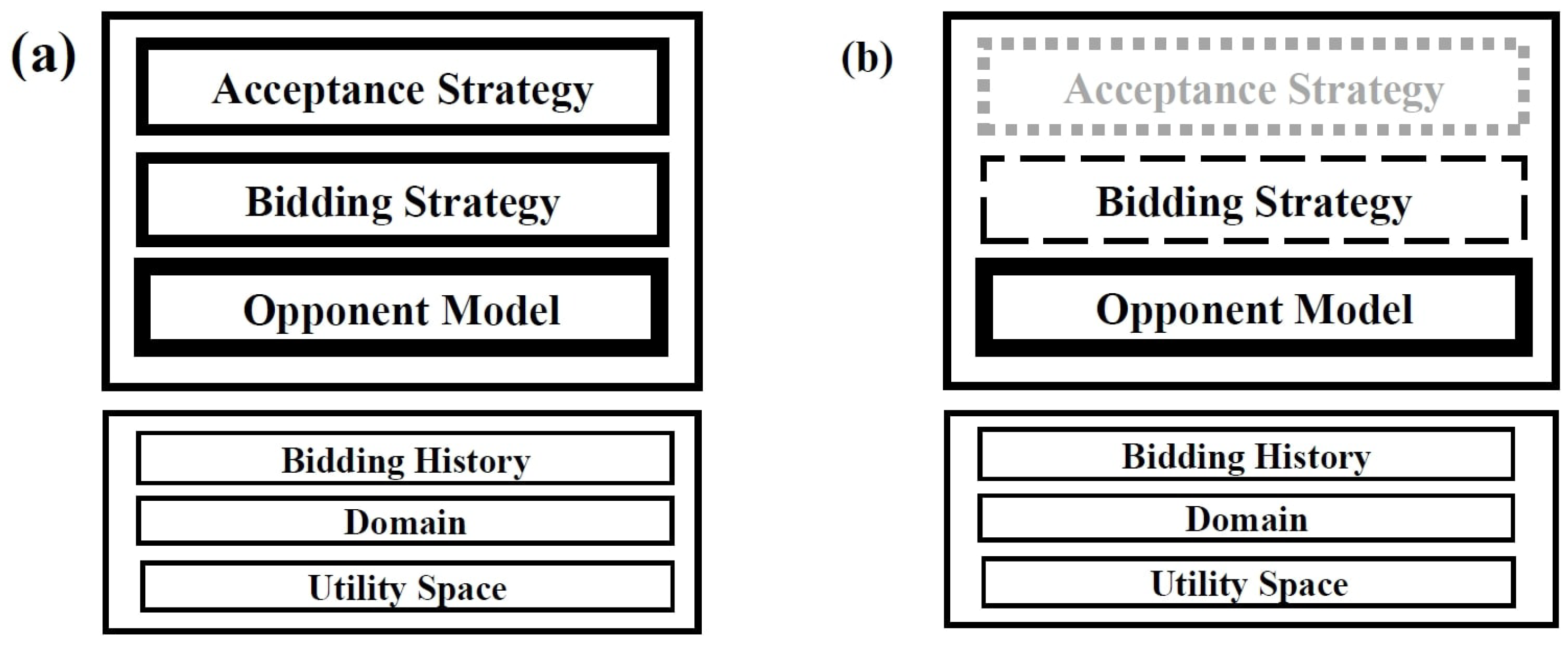
In an experimental analysis of modeling opponents, we require some benchmark agents that either (1) propose bids (B agents that assess the accuracy of the opponent model) or (2) propose bids while considering the acceptance or rejection of the opponent’s bids (BA agents that assess the performance of the opponent model). The latter benchmark agents can assess the performance of the agents once the negotiation ends. During the accuracy assessment, each benchmark agent has a B configuration comprising only a bidding strategy (see Figure 5a) and obeys a BA configuration comprising both a bidding strategy and an acceptance strategy (see Figure 5b); that is, the benchmark agent is devoid of an opponent model and must propose bids only to provide training data, which will be used by another agent analyzing an opponent model. It should be noted that both the bidding and acceptance strategies of the benchmark agent are affected by the selected single-peaked utility function.

4.3.1. Bidding Strategies of B and BA

To evaluate all opponent models under the same conditions, all models must be trained on the same set of bids. Thus, all benchmark agents must be armed with non-adaptive bidding strategies; otherwise, they will adapt to the behaviors of their opponents and violate the fairness of the experiments and their results. Following the POPPONENT experiments [24], the following three non-adaptive bidding strategies are utilized in this evaluation.
  • Concession strategies: In a concession strategy, the agent should start the negotiation with a bid having the highest utility and concede to a bid with the lowest utility (also called the reservation value). The target utility in a bidding concession strategy is calculated as
    U t = P max · 1 t 1 E ,
    where E is the concession rate and P max is the highest utility in the agent’s outlook. Here, we set E = 0.1 ,   1 ,   2 and P max = 1 .
  • Offset-based strategies: The target utility in an offset-based bidding strategy is calculated as described for a concession bidding strategy, but P max is not assigned with the highest utility. Here, we utilize a linear concession rate ( E = 1 ) and set P max = 0.7 ,   0.8 ,   0.9 .
  • Non-concession strategies: In a non-concession strategy, the agent starts the negotiation with a minimum utility P min and progress towards the highest utility P max = 1 over time. More specifically, the target utility in a non-concession bidding strategy is calculated as
    U t = P min + 1 P min · t ,
    where P min = 0.25 ,   0.5 ,   0.75 .

4.3.2. Acceptance Strategy of BA

To implement the acceptance strategy, we provide all benchmark agents with A C next , as popularly done in ANAC. Every agent armed with A C next accepts an opponent’s offer if the utility of that offer at least equals the utility of the benchmark agent’s ready-to-send bid. Note that any other rational acceptance strategy that gives more credit to higher utilities is also permitted.

4.4. Configuration of the Modeling Agent

The agents whose opponent models are under analysis receive their preference profiles from the utility function of the negotiation domain, as usually done in ANAC. All agents attend bilateral negotiations according to the Alternating Offers Protocol (AOP) [25]. Agents on both sides need a bidding strategy, by which they render a bid every time their turn approaches, and they obey the BO configuration illustrated in Figure 6a. During the evaluation, the agents on both sides lack an acceptance strategy, so all bilateral negotiations between the single-peaked and modeling agents progress until the deadline is reached. Consequently, the opponent models of the modeling agents are trained on the same number of bids, guaranteeing the fairness of both the training and comparison phases. After the negotiation, an agreement must be reached to obtain analyzable results for the performance analysis. These agents are configured as shown in Figure 6b.

4.4.1. Bidding Strategies of BO and BOA

The modeling agents must bid only to ensure the progress of the negotiations. What bids they render during the negotiations do not influence the analyses; accordingly, any bidding strategy is allowed. Moreover, as all BOA components compromise the agreement to some extent, we must deactivate the effect of the bidding and acceptance strategies on the performance measures. To this end, we simply set E = 0.1 ,   1 ,   2 (see Equation (6)).

4.4.2. Acceptance Strategy of BOA

Like the acceptance strategy of the BA agents (Section 4.3.2), the acceptance strategy of the BOA agents does not depend on the bids accepted by a modeling agent. So any rational acceptance strategy is acceptable. Here, we adopt A C next as the acceptance strategy of BOA agents.

5. Evaluation

This section evaluates whether the up-to-date opponent models can model the single-peaked opponents described in the previous section. We first describe the negotiation setting, negotiation domains, and opponent models under analysis. Finally, we specify the measures for evaluating the opponent models.

5.1. Negotiation Setting

The setting in this research is the prevailing setting of ANAC. Each year, the ANAC board adapts its rules to meet the intentions of the challenge. Accordingly, we use a selection of rules from the ANAC 2010–2019 challenge (see Table 5). The rules dictate the type of negotiation, deadline, domain, whether agents are allowed to learn in different sessions, and the value of the reservation. By aligning our research with the rules of ANAC, we ensure that our negotiation model is grounded in established principles and can be effectively compared with other state-of-the-art approaches in the field.

5.2. Negotiation Domains

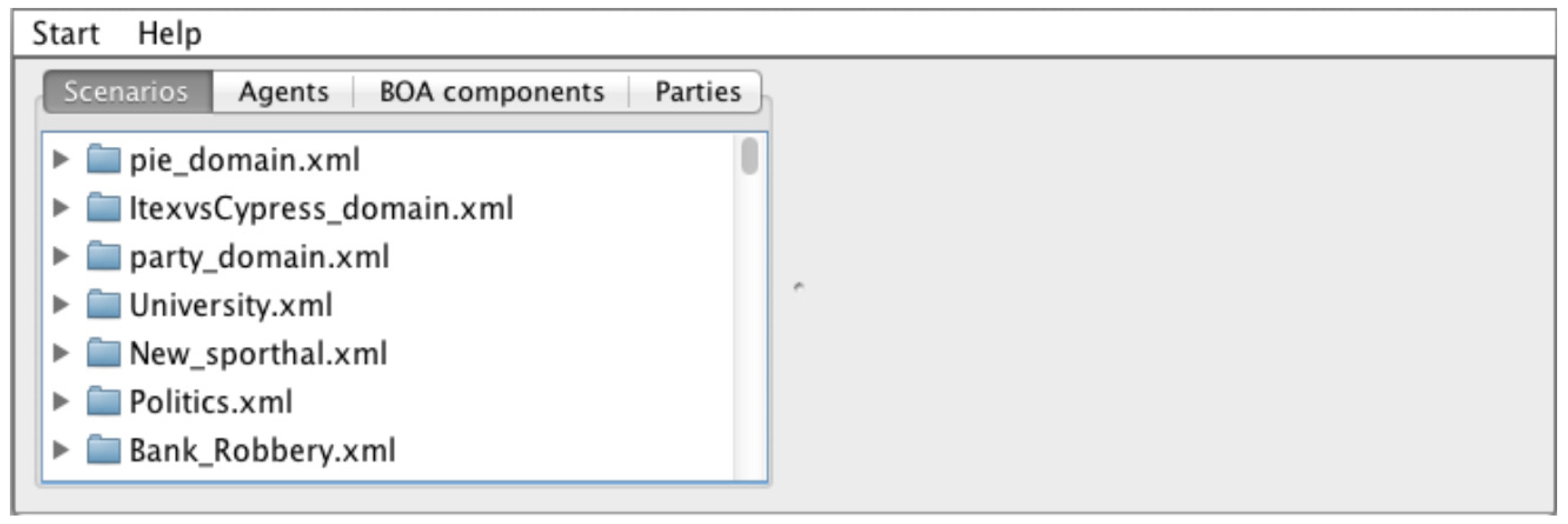
A negotiation domain includes all negotiation issues and their values. In this research, the domains are considered as common knowledge with variable sizes and subjects. Furthermore, the negotiation issues are linear; that is, they are independent and do not affect the utilities of each other. The single-peaked preferences are implemented as underlying utility functions that assign a proper utility to every negotiation item. To satisfy the definition and properties of single-peaked preferences, the issue(s) of the domains must be monotonic. For the present experiments, we extract seven domains with this property from the Genius repository [26]. Figure 7 presents a schematic representation of the GENIUS framework immediately following its initialization (refer to [27] for a comprehensive user guide for GENIUS). We also deactivate the discount factor’s effect ( D F = 1 ) and set R V = 0 . These seven domains are detailed below and are summarized in Table 6.
  • Barter: Within this small domain, specific amounts of three products (one with four values, one with five values, and another with four values) are exchanged. Therefore, 80 possible bids exist in this domain.
  • Itex vs. Cypress: Within this small domain, negotiations are made between the seller (a representative of the bicycle-component manufacturing firm Itex) and the buyer (Cypress). This domain consists of four issues: one with five values, one with four values, and two with three values. Thus, 180 bids are available in this domain.
  • Airport Site Selection: Within this medium-sized domain, the location of an airport is decided. This decision depends on three issues, one with ten values, one with seven values, and one with six values. The aggregate number of bids in this domain is 420.
  • Smart Energy Grid: Within this medium-sized domain, energy producers, consumers, and brokers engage in negotiations on four issues, each with five values. Therefore, 625 possible bids exist in this domain.
  • Pie: Within this medium-sized domain, negotiators consider the size of a piece of a pie. The number of possible bids equals the number of values in the issue (i.e., 1001).
  • Energy Small: Within this large domain, a representative of an electricity company negotiates with a representative of a wholesale buyer to reduce energy consumption during peak hours. This domain contains six issues with five values each, giving rise to 15625 available bids.
  • Energy: This domain resembles the Energy Small domain but is larger. More precisely, the Energy domain consists of eight issues, each with five values. Therefore, the aggregated number of bids is 390625.

5.3. Extracted Opponent Models

This paper estimates the preference profile (or utility function) of single-peaked opponents. Among the available opponent models, we strictly seek those that can estimate the preferences of opponents. Opponent models extracted from the Genius repository are of either the frequency or Bayesian category [28]. Bayesian models mainly generate a set of candidate preference profiles, which are gradually updated using the Bayes theorem under assumptions of the opponent’s bidding strategy. Finally, one of the preference profiles is acknowledged as the solution. Meanwhile, frequency-based opponent models estimate the opponent’s preference profile by calculating the frequency of issues and value changes in the received bids. We also evaluate two perceptron-based opponent models [24], which are claimed to be effective and accurate. The names, attendance dates, ranks, institutions, and countries of the selected opponent models are summarized in Table 7.

5.4. Evaluation Measures

The accuracy with which each opponent model can estimate its opponent’s preference profile was determined by the Pearson correlation. To evaluate the performances of the models, we employed five measures from ANAC [24]. These measures are described below.

5.4.1. Accuracy Measure

The Pearson correlation is a popular choice for accuracy evaluations of an opponent model. This measure calculates the similarity between the estimated utility and the real utility of a bid [24] as follows:
d p u OP , u OP = ω Ω u OP ω u OP ¯ u OP ω u OP ¯ ω Ω u OP ω u OP ¯ 2 ω Ω u OP ω u OP ¯ 2
where u OP and u OP denote the real and estimated preference profiles of the opponent, respectively, and u OP ω and u OP ω denote the actual and estimated utilities, respectively, of bid ω in the opponent’s preference profile. The Pearson correlation is a proper measure because it measures the accuracy of the opponent model in terms of the utility estimation of the bids from the opponent’s viewpoint (not the actual utilities).

5.4.2. Performance Measures

The performances of the opponent models are evaluated in terms of the following five ANAC measures.
  • The average individual utility [29] is calculated as
    AvgUtility A = i = 1 N utility A i N ,
    where N is the aggregate number of sessions, AvgUtility A denotes the average utility acquired by agent A during N negotiation sessions, and utility A i refers to the utility of agent A in session i.
  • The social welfare (also known as the average joint utility) of the agents is calculated as
    AvgJointUtility A , B = i = 1 N utility A i + utility B i 2 N ,
    where N is the total number of negotiation sessions, and AvgJointUtility A , B is the social welfare acquired by both agents during the N sessions. Moreover, utility A i and utility B i respectively denote the utilities of agents A and B in session i.
  • The average Nash distance of agreements [29] refers to the average distance of an agreement from the Nash point. It is calculated as follows:
    AvgNashDist A , B = i = 1 N NashDist A , B i N .
    In this expression,
    NashDist A , B i = utility A i NashUtility A i 2 + utility B i NashUtility B i 2 ,
    where AvgNashDist A , B is the average Nash distance of both opponents during the N negotiation sessions, NashDist A , B i denotes the Nash distance in session i, and NashUtility A i and NashUtility B i denote the utilities of agents A and B, respectively, at the Nash point within N sessions. Here, the Nash point is a unique point on the Pareto frontier where the multiplication of both agents’ utilities is maximized [30].
  • The average Pareto distance of agreements [29], which defines the smallest average distance between the achieved agreement and the Pareto frontier, is calculated as
    AvgParetoDist A , B = i = 1 N ParetoDist A , B i N .
    In Equation (13),
    ParetoDist A , B i = utility A i ParetoUtility A i 2 + utility B i ParetoUtility B i 2
    where AvgParetoDist A , B is the average distance of the acquired agreements of both opponents from the Pareto frontier within the N sessions, ParetoDist A , B i is the distance of the agreement from the Pareto frontier in session i, and ParetoUtility A i and ParetoUtility B i are the utilities of agents A and B, respectively, at their Pareto points in session i.
  • The average time to agreement determines the average time for reaching an agreement during N negotiation sessions. It is calculated as
    AvgTime = i = 1 N TimeOfAgreement i N ,
    where TimeOfAgreement i denotes the time for achieving an agreement in session i.

5.5. Experimental Settings

Experiments were conducted in two settings taken from POPPONENT’s experiments [24]. The agents were configured as illustrated in Figure 5 and Figure 6, and their components are summarized in Table 8. Briefly, 9 bidding strategies are combined with 18 single-peaked preference profiles to engender 162 single-peaked agents: 54 conceders, 54 offset-based agents, and 54 non-conceder agents. Conceder agents are predictable because they start the negotiation with their best bid, concede during the negotiation, and produce unique set bids. The other two categories are unpredictable because they neither initiate with their best bid nor concede. Among 33 opponent models (Table 7), 31 models (19 frequency-based, 8 Bayesian, and 4 classic models) were extracted from the Genius repository. The remaining two agents are perceptron-based. All four classic models (the No Model, Opposite Model, Perfect Model, and Worst Model) were utilized in the performance assessment experiment, but the Perfect and Worst models were excluded from the accuracy assessment because their accuracies invariably equal 1 and 1 , respectively.

5.6. Interactions of the Agents

The interactions among the modeler and single-peaked agents are shown in Figure 8. During the accuracy experiment, 31 modeler agents negotiated with 162 single-peaked agents. All opponent models were trained on seven scenarios (Section 5.2). Therefore, the number of executed negotiation sessions required for training each opponent model in 5000 rounds was 7 × 162 = 1134 . Each round consisted of two bids: (1) the offer of the modeler agent and (2) the counter-offer of the benchmark agent in response to the modeler agent. Therefore, 1134 × 5000 = 5,670,000 training bids were made by each opponent model. As 31 opponent models were employed in the experiment, there were 31 × 5,670,000 = 175,770,000 executed rounds and 2 × 175,770,000 = 351,540,000 exchanged offers.
During the performance experiment, 33 modeler agents negotiated on both sides (played two roles) in front of the single-peaked agents. This negotiation pattern avoids partiality in the results and (consequently) in the analyses. Hence, in 1000 rounds, each opponent model executed 7 × 2 × 162 = 2268 negotiation sessions. As each opponent model was armed with three bidding strategies, the total number of negotiation sessions was 2268 × 33 × 3 = 224,532 .

6. Results

We comprehensively analyzed the results of automated negotiations comprising 351540000 offers in the accuracy experiments and 449064000 offers in the performance experiments. The performance measures were those discussed in Section 5.4.1 and Section 5.4.2.

6.1. Experimental Results for Accuracy

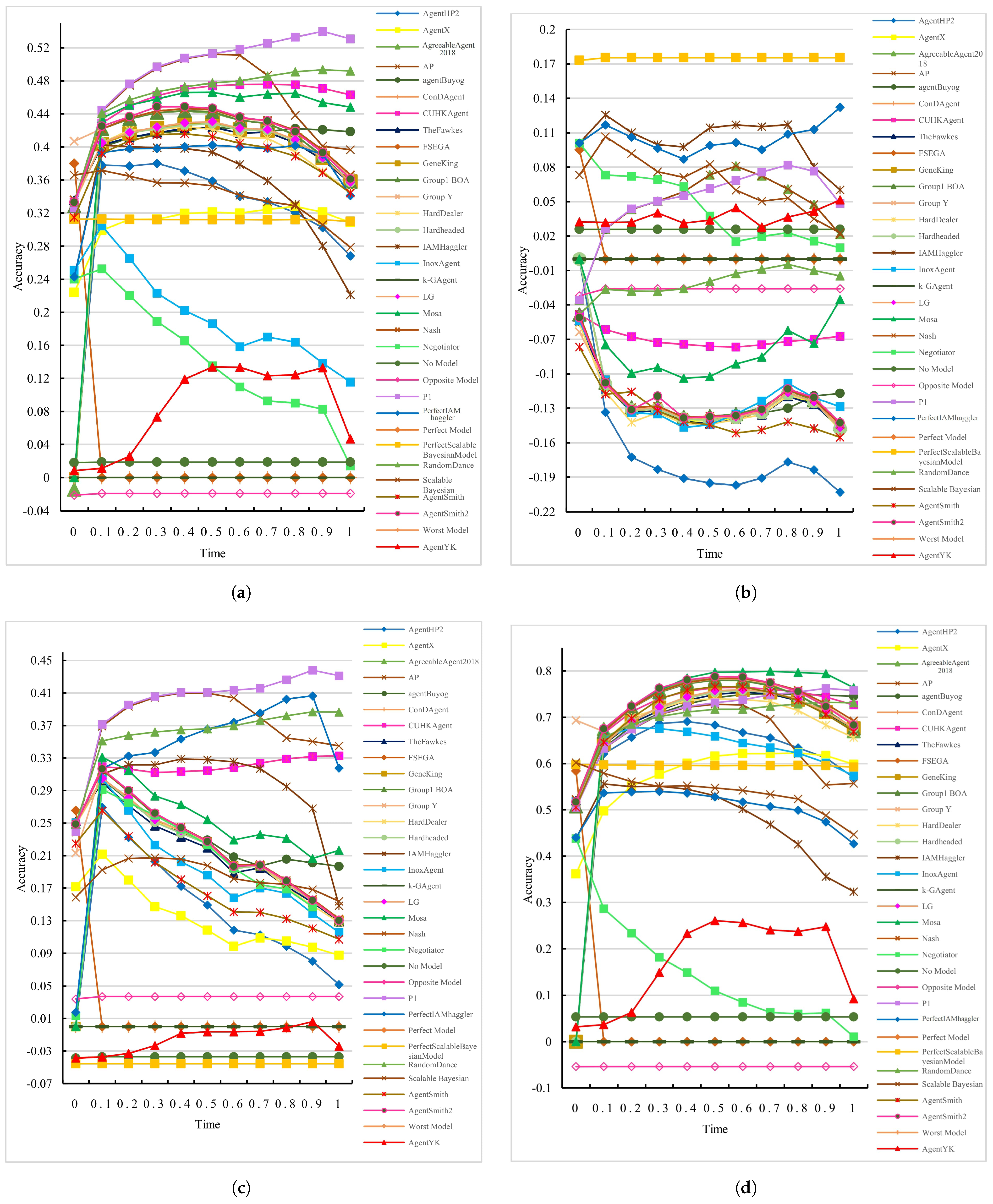
Our experimental analysis is delineated into two primary categories: (1) the utility function types utilized by the bidding agents—namely, Gaussian, skew-normal, and triangular—and (2) the domain sizes, which are classified as small, medium, and large. The empirical findings are depicted through a series of figures, each illustrating a distinct aspect of the analysis. Figure 9a aggregates the accuracy data across all utility functions and domain sizes, offering a consolidated perspective of the opponent models’ capabilities. Subsequently, Figure 9b–d focus on the models’ interactions with bidding agents employing Gaussian, skew-normal, and triangular utility functions, respectively. In parallel, we examine the influence of domain size on model accuracy, with Figure 10a representing small domains, Figure 10b for medium domains, and Figure 10c,d providing insights into the performance within large domains.
To evaluate the accuracy of each opponent model, we calculated the Pearson correlation between the estimated and actual utilities, splitting the normalized negotiation deadline into 11 equal intervals. The FSEGA and AgentSmith opponent models could not be executed in the Energy domain. The perceptron-based model P1 achieved the highest accuracy, which also increased over time (Figure 9a). The other perceptron-based model AP achieved the second-highest accuracy, which increased up to t = 0.5 . Obviously, t = 0.5 was a critical time at which the accuracy of most opponent models either continued to increase or began to decline. It was concluded that models with decreasing accuracy did not properly use their last received bids. This behavior tended to prevail in the Bayesian opponent models, which rely on hypotheses regarding the opponent’s bidding strategy. Indeed, Figure 9b shows that none of the opponent models performed satisfactorily when confronting the Gaussian opponents, and most of the models exhibited fluctuating accuracy. The functionality improved in the Bayesian models and was weakest in the frequency models.
When faced with skew-normal opponents, P1 and AP (to some extent) were the most accurate models (Figure 9c). Comparing the results of Figure 9b,c, one observes that skew-normal opponents greatly improved the functionalities of the opponent models. However, the accuracies of the opponent models usually decreased over time. Meanwhile, when the opponent models confronted general triangular opponents (Figure 9d), their accuracies were largely improved in general and from those of the previous categories. This is probably because the triangular function’s piece-wise linearity implies a simpler structure, which may inherently facilitate more accurate estimation. Conversely, the Gaussian function, despite its regularity, has a continuous curvature that can introduce complexities in estimation, especially if the estimation method is not specifically tailored to capture such nuances. The most- and least-accurate opponent models were the frequency and Bayesian models, respectively.
The accuracies of the opponent models over seven domains of different sizes are presented in Figure 10a–d. As shown in Figure 10a, the opponent models confronting the benchmark opponents performed more accurately on large domains than on medium and small domains. Moreover, the accuracy on medium domains exceeded that on small domains. The numerous possible bids on large domains provide more opportunities for convergence to an accurate preference profile by each opponent model. When confronting Gaussian opponents, the opponent models performed most accurately on medium-sized domains and least accurately on small domains (Figure 10b). Confronted with skew-normal opponents, the opponent models showed similar accuracies on the large and medium domains and lower accuracies on the small domains (Figure 10c). On the contrary, when confronting general triangular opponents, the accuracies of the opponent models were quite similar on the small, medium, and large domains (Figure 10d) but were nonetheless highest on the large domain and weakest on the medium domain. The most accurate model in each category is summarized in Table 9.

6.2. Experimental Results for Performance

Under the setting of the performance experiment (Section 4.4 and Section 5.4.2), all 33 opponent models were negotiated in front of 162 opponents, and their performances were evaluated in terms of average individual utility, social welfare, Nash distance, Pareto distance, and agreement-reaching time. As the FSEGA and CondAgent opponent models could not be executed in the Energy domain, they were evaluated in six domains. The performance results of the opponent models confronting all, Gaussian, skew-normal, and general triangular opponents are compared in Figure 11a–d. The opponent models achieving the highest performance measures against these four categories of benchmark bidding agents are summarized in the first, second, third, and fourth parts of Table 10, respectively. The individual utility and social welfare performances of the opponent models were highest against Gaussian opponents, followed by skew-normal and general triangular opponents (Figure 11a–d). Conversely, the Nash distance performances of the opponent models were maximized against general triangular opponents, followed by skew-normal and Gaussian opponents. The Pareto distance and temporal metrics data showed no discernible patterns, and the outcomes were comparable among the models.

6.3. Key Findings

The findings for the accuracy as well as performance experiments on 31 opponent models are summarized below.
  • Let A i be the accuracy of the opponent models in category i, and let Gaussian, Skew, and Triangular represent the Gaussian, skew-normal, and triangular benchmark agents, respectively. Referring to Figure 9b–d, we can see that the accuracies of the opponent models in modeling the utility function (underlying the preference profile) of the benchmark single-peaked agents are as follows:
    A Triangular > A Skew > A Gaussian
    This suggests that the opponent models are more accurate at estimating utility functions that are simpler and less complex, as represented by the triangular distribution, compared to the more complex skew-normal and Gaussian distributions. This leads to the following proposition:
    Proposition 1
    (Total Accuracy). Raising the degree of the benchmark agents’ utility function (from triangular to skew-normal to Gaussian) encumbers the accurate estimation of the utility function by the opponent models and reduces their accuracies.
  • Let A i be the accuracy of an opponent model in a size-i domain, and let S, M, and L denote small, medium, and large domains, respectively.
    The accuracies of the opponent models in modeling the utility functions of all benchmark agents (Figure 10a) decrease as the domain size increases. Specifically, the accuracy is highest in large domains, followed by medium domains, and it is lowest in small domains:
    A L > A M > A S
    Separating the benchmark agents into Gaussian, skew-normal, and general triangular and referring to Figure 10b–d, respectively, the accuracies A i j of the opponent models confronting all benchmark agents of type i in a size-j domain are ordered as follows:
    A = A i M > A i L > A i S , i = Gaussian A i L > A i M > A i S , i = Skew A i L > A i S > A i M , i = Triangular
    This does not show any specific association between the degree of the utility function and the size of the domain it is negotiating on.
  • Now suppose that I U i , S W i , and N D i respectively signify the individual utility, social welfare, and Nash distance of the opponent models in category i, and that Gaussian, Skew, and Triangular correspond to the Gaussian, skew-normal, and triangular benchmark agents, respectively. From Figure 11a–c, it follows that the performances of the opponent models in each category is as follows:
    I U Gaussian > I U Skew > I U Triangular ,
    S W Gaussian > S W Skew > S W Triangular ,
    N D Triangular > N D Skew > N D Gaussian ,
    leading to the following proposition:
Proposition 2
(Performance Metrics). When the degree of the utility function increases (from triangular to skew-normal to Gaussian), the individual utility and social welfare of the opponent models do not decrease; instead, they increase. This indicates that despite the increased complexity of the utility function, it does not impede the opponent models from reaching agreements that enhance their individual utility and social welfare. However, this increased complexity results in a worsening of the Nash distance.
Table 11 states the total number of top performances achieved by each opponent model in each performance category. Randomdance most commonly maximized the social welfare, Pareto efficiency, and Nash distance, whereas CUHKAgent and P1 outperformed the other opponents on individual utility and agreement-reaching time, respectively.

7. Conclusions

In automated negotiation, agents offer bids to complete tasks that satisfy the attitudes and strategies of their owners. Each agent constructs an opponent model to estimate information on the opponent and to hence raise its chance of success. However, despite their omnipresence, single-peaked preferences have received little attention in automated negotiations. We analyzed the efficacy and accuracy of opponent models in front of various single-peaked agents. All opponent models were extracted from agents in the Genius repository and were equipped with proper components for negotiating with single-peaked benchmark agents. In the accuracy assessment, the perceptron-based models P1 and AP outperformed the other opponent models, but their accuracy was deficient in some categories. In the performance evaluation, the frequency opponent model Randomdance surpassed the other models in social welfare, Pareto efficiency, and Nash distance, whereas CUHKAgent was the top performer in individual utility, and P1 improved the time-to-agreement in most categories.
The created single-peaked agents are suitable benchmarks for future studies. The opponent models were much less accurate against Gaussian benchmark agents than against skew-normal and triangular benchmark agents. Therefore, Gaussian benchmark agents should be meticulously investigated to understand why they degrade the accuracy of their opponents. For instance, one could evaluate the accuracies of the opponent models after dividing the benchmark agents into categories based on their symmetries or asymmetries. A new opponent model with resilience against different opponents with different bidding strategies might also yield superior results.
Finally, when modeling single-peaked opponents, the most successful agents can provide insights into forecasting peaks in financial markets.

Author Contributions

Conceptualization, F.H. and F.N.-M.; Data curation, F.H. and F.N.-M.; Formal analysis, F.H., F.N.-M., and K.F.; Investigation, F.H.; Methodology, F.H. and F.N-M.; Software, F.H. and F.N-M.; Supervision, F.N.-M. and K.F.; Validation, F.N.-M. and K.F.; Visualization, F.H. and F.N.-M.; Writing—original draft, F.H.; Writing—review and editing, F.N.-M. and K.F. All authors have read and agreed to the published version of the manuscript.

Funding

This research received no external funding.

Institutional Review Board Statement

Not applicable.

Informed Consent Statement

Not applicable.

Data Availability Statement

All domains and all preference profiles utilized in the present research are available in the Genius repository version 9.11 [31]. All 162 benchmark agents produced in this study are available at https://github.com/hsnvnd/Benchmark_Agents (accessed on 22 July 2024). The details of the automated negotiations comprising 351540000 and 449064000 offers exchanged in the accuracy and performance experiments, respectively, are available at https://github.com/hsnvnd/Performance_and_Accuracy_logs (accessed on 22 July 2024).

Conflicts of Interest

The authors declare no conflicts of interest.

References

  1. Bazerman, M.H.; Curhan, J.R.; Moore, D.A.; Valley, K.L. Negotiation. Annu. Rev. Psychol. 2000, 51, 279–314. [Google Scholar] [CrossRef] [PubMed]
  2. Paliwal, P.; Webber, J.L.; Mehbodniya, A.; Haq, M.A.; Kumar, A.; Chaurasiya, P.K. Multi-agent-based approach for generation expansion planning in isolated micro-grid with renewable energy sources and battery storage. J. Supercomput. 2022, 78, 18497–18523. [Google Scholar] [CrossRef]
  3. Faratin, P.; Sierra, C.; Jennings, N.R. Negotiation decision functions for autonomous agents. Robot. Auton. Syst. 1998, 24, 159–182. [Google Scholar] [CrossRef]
  4. Shields, D.J.; Tolwinski, B.; Kent, B.M. Models for conflict resolution in ecosystem management. Socio-Econ. Plan. Sci. 1999, 33, 61–84. [Google Scholar] [CrossRef]
  5. Yang, M.; Zhang, A.; Bi, W.; Wang, Y. A resource-constrained distributed task allocation method based on a two-stage coalition formation methodology for multi-UAVs. J. Supercomput. 2022, 78, 10025–10062. [Google Scholar] [CrossRef]
  6. Gao, J.; Wong, T.; Wang, C. Coordinating patient preferences through automated negotiation: A multiagent systems model for diagnostic services scheduling. Adv. Eng. Inform. 2019, 42, 100934. [Google Scholar] [CrossRef]
  7. Benatia, I.; Laouar, M.R.; Eom, S.B.; Bendjenna, H. Incorporating the negotiation process in urban planning DSS. Int. J. Inf. Syst. Serv. Sect. (IJISSS) 2016, 8, 14–29. [Google Scholar] [CrossRef]
  8. Nassiri-Mofakham, F.; Huhns, M.N. Role of culture in water resources management via sustainable social automated negotiation. Socio-Econ. Plan. Sci. 2023, 86, 101465. [Google Scholar] [CrossRef]
  9. Luo, J.; Wang, G.; Li, G.; Pesce, G. Transport infrastructure connectivity and conflict resolution: A machine learning analysis. Neural Comput. Appl. 2022, 34, 6585–6601. [Google Scholar] [CrossRef]
  10. ANAC. Available online: http://ii.tudelft.nl/negotiation/node/7 (accessed on 22 July 2024).
  11. Dirkzwager, A. Towards Understanding Negotiation Strategies: Analyzing the Dynamics of Strategy Components. Master’s Thesis, Delft University of Technology, Delft, The Netherlands, 2013. [Google Scholar]
  12. Fatima, S.; Kraus, S.; Wooldridge, M. The Negotiation Game. IEEE Intell. Syst. 2014, 29, 57–61. [Google Scholar] [CrossRef]
  13. Hassanvand, F.; Nassiri-Mofakham, F. Experimental analysis of automated negotiation agents in modeling Gaussian bidders. In Proceedings of the 2021 12th International Conference on Information and Knowledge Technology (IKT), Babol, Iran, 14–16 December 2021; pp. 197–201. [Google Scholar]
  14. Hassanvand, F.; Nassiri-Mofakham, F. Automated Negotiation Agents in Modeling Gaussian Bidders. AUT J. Model. Simul. 2023, 55, 3–16. [Google Scholar]
  15. Ito, T.; Klein, M. A multi-issue negotiation protocol among competitive agents and its extension to a nonlinear utility negotiation protocol. In Proceedings of the fifth International Joint Conference on Autonomous Agents and Multiagent Systems, Hakodate, Japan, 8–12 May 2006; pp. 435–437. [Google Scholar]
  16. Booth, R.; Chevaleyre, Y.; Lang, J.; Mengin, J.; Sombattheera, C. Learning conditionally lexicographic preference relations. In Proceedings of the ECAI, Amsterdam, The Netherlands, 4 August 2010; Volume 10, pp. 269–274. [Google Scholar]
  17. Chari, K.; Agrawal, M. Multi-issue automated negotiations using agents. INFORMS J. Comput. 2007, 19, 588–595. [Google Scholar] [CrossRef]
  18. Martínez-Mora, F.; Puy, M.S. Asymmetric single-peaked preferences. BE J. Theor. Econ. 2012, 12, 0000101515193517041941. [Google Scholar] [CrossRef]
  19. Varian, H.R. A Bayesian approach to real estate assessment. Stud. Bayesian Econom. Stat. Honor. Leonard Savage 1975, 195–208. [Google Scholar]
  20. Christoffersen, P.F.; Diebold, F.X. Optimal prediction under asymmetric loss. Econom. Theory 1997, 13, 808–817. [Google Scholar] [CrossRef]
  21. Surico, P. The Fed’s monetary policy rule and US inflation: The case of asymmetric preferences. J. Econ. Dyn. Control 2007, 31, 305–324. [Google Scholar] [CrossRef]
  22. Waud, R.N. Asymmetric policymaker utility functions and optimal policy under uncertainty. Econom. J. Econom. Soc. 1976, 53–66. [Google Scholar] [CrossRef]
  23. Marchenko, Y.V.; Genton, M.G. A suite of commands for fitting the skew-normal and skew-t models. Stata J. 2010, 10, 507–539. [Google Scholar] [CrossRef]
  24. Zafari, F.; Nassiri-Mofakham, F. Popponent: Highly accurate, individually and socially efficient opponent preference model in bilateral multi issue negotiations. Artif. Intell. 2016, 237, 59–91. [Google Scholar] [CrossRef]
  25. Rubinstein, A. Perfect equilibrium in a bargaining model. Econom. J. Econom. Soc. 1982, 97–109. [Google Scholar] [CrossRef]
  26. Hindriks, K.; Jonker, C.M.; Kraus, S.; Lin, R.; Tykhonov, D. Genius: Negotiation environment for heterogeneous agents. In Proceedings of the 8th International Conference on Autonomous Agents and Multiagent Systems-Volume 2, Budapest, Hungary, 10–15 May 2009; pp. 1397–1398. [Google Scholar]
  27. Baarslag, T.; Pasman, W.; Hindriks, K.; Tykhonov, D. Using the Genius Framework for Running Autonomous Negotiating Parties. 2019. Available online: https://ii.tudelft.nl/genius/sites/default/files/userguide.pdf (accessed on 22 July 2024).
  28. Nazari, Z.; Lucas, G.M.; Gratch, J. Opponent modeling for virtual human negotiators. In Proceedings of the Intelligent Virtual Agents: 15th International Conference, IVA 2015, Delft, The Netherlands, 26–28 August 2015; Proceedings 15. Springer: Berlin/Heidelberg, Germany, 2015; pp. 39–49. [Google Scholar]
  29. Hindriks, K.; Jonker, C.M.; Tykhonov, D. Negotiation dynamics: Analysis, concession tactics, and outcomes. In Proceedings of the 2007 IEEE/WIC/ACM International Conference on Intelligent Agent Technology (IAT’07), Silicon Valley, CA, USA, 2–5 November 2007; pp. 427–433. [Google Scholar]
  30. Weiss, G. Multiagent systems: A modern approach to distributed artificial intelligence. Int. J. Comput. Intell. Appl. 2001, 1, 331–334. [Google Scholar]
  31. ANAC. Genius. Available online: https://tracinsy.ewi.tudelft.nl/pub/svn/Genius/ (accessed on 22 July 2024).
Figure 1. Representations of shortfall (curve fitted to the green squares) and excess avoidance (curve fitted to the purple triangles).
Information 15 00508 g001
Figure 2. Skew-normal utility functions applied in this paper, plotted over the Pie domain.
Information 15 00508 g002
Figure 3. Gaussian utility functions used in this paper, plotted over the Pie domain.
Information 15 00508 g003
Figure 4. General triangular utility functions used in this paper, plotted over the Pie domain.
Information 15 00508 g004
Figure 5. Configuration for evaluating the opponent model of a rival: (a) B benchmark agent for accuracy assessment; (b) BA benchmark agent for performance assessment [13].
Information 15 00508 g005
Figure 6. Configuration of the rivals: (a) BO agent for the accuracy assessment and (b) BOA agent for the performance assessment [13].
Information 15 00508 g006
Figure 7. Initial interface of GENIUS, showcasing the components panel on the left and the status panel on the right [27].
Information 15 00508 g007
Figure 8. Interactions between the modeling agents (Side 1) and benchmark agents (Side 2) during (a) the performance assessment and (b) the accuracy assessment [13].
Information 15 00508 g008
Figure 9. Accuracies of the opponent models in front of (a) all benchmark agents; (b) Gaussian agents; (c) skew-normal agents; (d) general triangular agents.
Information 15 00508 g009
Figure 10. Accuracies of the opponent models for different domain sizes in front of (a) all benchmark agents; (b) Gaussian agents; (c) skew-normal agents; (d) general triangular agents.
Information 15 00508 g010
Figure 11. Performance results of the opponent models confronting all benchmark agents (black), Gaussian agents (cyan), skew-normal agents (green), and general triangular agents (red): (a) Individual utility; (b) Social welfare; (c) Nash distance; (d) Pareto distance; (e) Time to agreement.
Information 15 00508 g011
Table 1. Parameters of the skew-normal agents.
Type123456
Name S_Left_HalfNeg S_Left_HalfS_MiddleNeg S_MiddleS_Right_HalfNeg S_Right_Half
Parameter ω 0.010.010.0050.0050.040.04
pFirst valueFirst valueMedianMedianLast valueLast value
α + 10 10 + 20 20 15 + 15
Table 2. Parameters of the Gaussian agents.
Type123
NameLeft_HalfRight_HalfMiddle
Parameter ω 0.010.040.005
pFirst valueLast valueMedian
Table 3. Parameters of the general triangular agents.
Type123456789
NameTri70_30_P3Tri70_30_P1Tri70_30_P0.5Tri20_20_P3Tri20_20_P1Tri20_20_P0.5Tri1_90_P3Tri1_90_P1Tri1_90_P0.5
ParameterL707070202020111
R303030202020909090
pMedianMedianMedianMedianMedianMedianMedianMedianMedian
λ 303030202020909090
h111111111
Table 4. Notations used in Algorithms 1–3.
NotationDescription
IssuesAll issues in the domain
issueOne issue in Issues
D_coCopy of the domain
F_nameFunction name selected by user
vAn issue value
pPeak
ω Scale
α Shape
hShape height
RRight minimum
LLeft minimum
λ Power
Table 5. Summary of the rules of encounter adopted in the present study.
Negotiation TypeMulti-Issue Bilateral
DeadlineCommon Knowledge and Round-Based
Domain TypeLinear
Learning Between SessionsNo
Reservation Value1
Table 6. Summary of the domains used in the present paper.
Domain NameDomain Size (Issues, Bids)
BarterSmall (3, 80)
Itex vs. CypressSmall (4, 180)
Airport Site SelectionMedium (3, 420)
PieMedium (1, 1001)
Smart Energy GridMedium (4, 625)
Energy SmallLarge (6, 15, 625)
EnergyLarge (8, 390, 625)
Table 7. Details of the opponent models extracted from ANAC 2010–2019.
#Agent NameCountryInstitutionYearRankOpponent
Model Type
1Perfect IAMHaggler----Bayesian
2Nash----Frequency
3Scalable Bayesian----Bayesian
4Perfect Scalable Bayesian----Bayesian
5AgentSmithThe NetherlandsTU Delft20107F 1Frequency
6IAMHagglerEnglandUniversity of Southampton20104FBayesian
7HardheadedThe NetherlandsTU Delft20111FFrequency
8CUHKAgentChinaThe University of Hong Kong20121FFrequency
9AgentLGIsraelBar-Ilan University20122FFrequency
10AgentXThe NetherlandsTU Delft201213Q 2Frequency
11NegotiatorThe NetherlandsTU Delft20123FBayesian
12TheFawkesThe NetherlandsTU Delft20131FFrequency
13InoxAgentThe NetherlandsTU Delft20136QFrequency
14k-GAgentJapanTokyo University of Agriculture and Technology20147FFrequency
15AgentYKJapanShizuoka University20148FFrequency
16APIranUniversity of Isfahan2014-Perceptron
17P1IranUniversity of Isfahan2014-Perceptron
18RandomDanceJapanTokyo University of Agriculture and Technology20153FFrequency
19agentBuyogSingaporeNanyang Technological University20155FFrequency
20AgentHP2JapanTokyo University of Agriculture and Technology201610FFrequency
21AgentSmith2The NetherlandsTU Delft201616FFrequency
22GeneKingJapanNagoya University20176FFrequency
23MosaUSASouthwest University20177FFrequency
24AgreeableAgent2018IranUniversity of Tehran20181FFrequency
25Group YTurkeyOzyegin University20186FFrequency
26ConDAgentGreeceUniversity of Crete20188FBayesian
27FSEGARomaniaBabeş–Bolyai University20192FBayesian
28Group1 BOA--201911FFrequency
29HardDealer--20195FBayesian
30No Model----Classic
31Perfect Model----Classic
32Worst Model----Classic
33Opposite Model----Classic
1 F: final round; 2 Q: qualifying round
Table 8. Components of the modeler (rival) and bidder (benchmark) agents in the accuracy and performance experiments.
ExperimentComponents/
Negotiating Agent
Single-Peaked
Preference Profile
Bidding
Strategy
Acceptance
Strategy
Opponent
Model
AccuracyModeler
Bidder
PerformanceModeler
Bidder
Table 9. Most accurate model for each domain size when faced with different benchmark agents.
Benchmark AgentDomain SizeThe Most Accurate ModelAccuracy
AllSmallPerfect Scalable Bayesian0.386888
MediumCUHKAgent0.488432
LargeCUHKAgent0.608656
GaussianSmallPerfect Scalable Bayesian0.268901
MediumIAMhaggler Bayesian0.216265
LargePerfect Scalable Bayesian0.269562
Skew-NormalSmallPerfect IAMhaggler Bayesian0.188162
MediumP10.455543
LargeCUHKAgent0.577745
General TriangularSmallRandomdance0.762287
MediumGroupy0.680891
LargeGroupy0.835907
Table 10. Top-performing models in each performance category when confronting single-peaked bidding agents.
Top Model *Measure
Opponent Individual Utility Social Welfare Pareto Distance Time Nash Distance
(1) 0.796499:
FSEGA
1.518985:
CondAgent
0.010909:
FSEGA
0.130557:
P1
0.238543:
Randomdance
(1) 0.794041:
CUHKAgent
1.518306:
Randomdance
0.017778:
Randomdance
0.130557:
P1
0.238543:
Randomdance
(2) 0.886457:
AP, P1
1.741716:
AP, P1
0.011423:
FSEGA
0.047787:
P1
0.128945:
Randomdance
(2) 0.886457:
AP, P1
1.741716:
AP, P1
0.013247:
Randomdance
0.047787:
P1
0.128945:
Randomdance
(3) 0.829467:
CUHKAgent
1.591632:
CondAgent
0.014377:
FSEGA
0.083414:
P1
0.187083:
Randomdance
(3) 0.829467:
CUHKAgent
1.589593:
Randomdance
0.016933:
Randomdance
0.083414:
P1
0.187083:
Randomdance
(4) 0.741977:
CUHKAgent
1.399601:
CondAgent
0.008426:
FSEGA
0.189577:
P1
0.309383:
Randomdance
(4) 0.741977:
CUHKAgent
1.397974:
Randomdance
0.017757:
AgentX, Group1, HardDealer, Hardheaded, IAMhaggler Bayesian, Inox, LG, Negotiator, Opposite Model, Perfect IAMhaggler Bayesian, Perfect Model, Perfect Scalable Bayesian, Scalable Bayesian, Smith1, Smith2, Worst Model
0.189577:
P1
0.309383:
Randomdance
* (1) All benchmark, (2) Gaussian, (3) skew-normal, and (4) general triangular bidding agents. exclusion of FSEGA and CondAgent (FSEGA and CondAgent could not be executed in the Energy domain).
Table 11. Total number of top performances of each model in each performance category.
#Agent NameNash
Distance
Average
Time
Pareto
Distance
Social
Welfare
Individual
Utility
1Perfect IAMHaggler201027
2Nash20927
3Scalable Bayesian40914
4Perfect Scalable Bayesian201027
5AgentSmith211027
6IAMHaggler50937
7Hardheaded201027
8CUHKAgent308312
9AgentLG201027
10AgentX201017
11Negotiator30937
12TheFawkes10101
13InoxAgent201027
14k-GAgent11000
15AgentYK00001
16AP34595
17P1430595
18RandomDance22014169
19agentBuyog60321
20AgentHP242321
21AgentSmith2201027
22GeneKing63443
23Mosa60321
24AgreeableAgent63321
25Group Y64322
26ConDAgent60351
27FSEGA201322
28Group1 BOA201027
29HardDealer201027
30No Model42321
31Perfect Model201127
32Worst Model201025
33Opposite Model30938
Disclaimer/Publisher’s Note: The statements, opinions and data contained in all publications are solely those of the individual author(s) and contributor(s) and not of MDPI and/or the editor(s). MDPI and/or the editor(s) disclaim responsibility for any injury to people or property resulting from any ideas, methods, instructions or products referred to in the content.