Abstract
SimRank is a widely used metric for evaluating vertex similarity based on graph topology, with diverse applications such as large-scale graph mining and natural language processing. The objective of the single-source and top-k SimRank query problem is to retrieve the kvertices with the largest SimRank to the source vertex. However, existing algorithms suffer from inefficiency as they require computing SimRank for all vertices to retrieve the top-k results. To address this issue, we propose an algorithm named HitSimthat utilizes a branch and bound strategy for the single-source and top-k query. HitSim initially partitions vertices into distinct sets based on their shortest-meeting lengths to the source vertex. Subsequently, it computes an upper bound of SimRank for each set. If the upper bound of a set is no larger than the minimum value of the current top-k results, HitSim efficiently batch-prunes the unpromising vertices within the set. However, in scenarios where the graph becomes dense, certain sets with large upper bounds may contain numerous vertices with small SimRank, leading to redundant overhead when processing these vertices. To address this issue, we propose an optimized algorithm named HitSim-OPT that computes the upper bound of SimRank for each vertex instead of each set, resulting in a fine-grained and efficient pruning process. The experimental results conducted on six real-world datasets demonstrate the performance of our algorithms in efficiently addressing the single-source and top-k query problem.
1. Introduction
In various real-world scenarios, the measurement of similarity between entities is often crucial. For instance, in recommendation systems, predicting potential friendships based on the similarity between individuals in a social network [1,2]; or recommending items to users based on their behavior and preferences [3]. In security systems, analyzing email similarity to detect spam messages [4]; or analyzing account similarity to identify fraudulent transactions [5]. Among existing similarity computation methods, those based on entity linkage relationships are most commonly employed. Among these, SimRank is a widely used model for computing vertex similarity based on the directed graph topology. SimRank was introduced by Jeh and Widom [6] in 2002, and it is formulated based on two intuitive statements: (1) If two entities (vertices) are referenced by similar entities (i.e., in a directed graph, if the in-neighbors of two different vertices are similar or identical), then those two entities are also considered similar, and (2) an entity is most similar to itself. The classical algorithm, named power method [6], along with its variations [7], serves as the foundation for computing SimRank between each two vertices. However, these algorithms suffer from the time and space complexity of , where n represents the total number of vertices in the graph G, as there exist vertex pairs in G. To tackle this challenge, Ref. [8] proposed the single-source and top-k query problem. This problem focuses on efficiently retrieving the k vertices with the largest SimRank to a specific source vertex. Existing approaches [8,9,10,11,12,13,14,15,16] for the single-source and top-k query problem primarily utilize the random walk method, resulting in notable improvements in both time and space efficiency. Ref. [10] proposed two heuristic algorithms employing truncated random walk and prioritized propagation strategies. Ref. [11] devised an index for SimRank computation based on -walk, despite the notable overhead in terms of space and preprocessing. Ref. [12] proposed an index-free algorithm named ProbeSim that outperforms the index-based approaches. The state-of-the-art algorithm CrashSim [13] improves the computational efficiency of SimRank in ProbeSim by truncating walk lengths.
Challenges. In the single-source and top-k query problem, existing approaches require computing the SimRank for all the vertices and subsequently sorting the top-k results in descending order based on their SimRank. However, computing SimRank for vertices requires sampling a large number of random walks, which is a time-consuming operation. Moreover, in real-world applications, the desired result scale k specified by users is often much smaller than the vertex scale n of the network. Therefore, computing SimRank for vertices with negligible SimRank value is redundant.
Our approach. Motivated by the above observations, we propose a novel algorithm called HitSim for the single-source and top-k query problem, which employs a branch and bound strategy. Specifically, by leveraging the inherent property that the SimRank of a vertex will decrease as its meeting length increases, HitSim partitions vertices into distinct sets based on their shortest-meeting lengths (Definition 5) and computes the upper bound of SimRank for each set. To reduce the redundant computation for the vertices with negligible SimRank, HitSim preferentially processes the vertices within the set with a larger upper bound. If the upper bound of a set is less than the minimum SimRank of the current results, the vertices within the set can be efficiently pruned in batch.
However, in scenarios where the graph becomes dense, the number of vertices within the same set can grow rapidly. This may result in a scenario where vertices with the same shortest-meeting lengths but significantly different SimRank are partitioned into the same set. Consequently, the efficiency will decrease since the algorithm may preferentially process the vertices with the shortest-meeting lengths but with a small SimRank. To address this issue of inefficient pruning in HitSim, we propose an optimized algorithm called HitSim-OPT. HitSim-OPT computes the upper bound of SimRank for each vertex, allowing for fine-grained pruning of vertices. Similar to HitSim, HitSim-OPT maintains the minimum SimRank of the current top-k results and prunes unpromising vertices by comparing their upper bounds with the minimum value. Our contributions are as follows:
- We propose an efficient algorithm, named HitSim, based on a branch and bound strategy to answer the single-source and top-k query. HitSim can efficiently prune the unpromising vertices within a set in batch, reducing redundant computation and improving overall efficiency.
- We further propose an optimized algorithm, named HitSim-OPT. By computing the upper bound of SimRank for each vertex, HitSim-OPT performs a fine-grained pruning strategy, resulting in further improvements in efficiency.
- We conduct experiments on six real-world datasets. The experimental results show that our algorithms can efficiently answer the single-source and top-k query.
Organization. The rest of this paper is summarized as follows. Section 2 provides some preliminaries. In Section 3, we give a review of existing works. In Section 4, we propose an efficient algorithm based on a branch and bound strategy for the single-source and top-k query. In Section 5, we further propose an optimized algorithm. Section 6 shows the experimental results. Section 7 concludes this paper.
2. Preliminaries
In this section, we formally introduce the notation and definitions. Mathematical notations used throughout this paper are summarized in Table 1.

Table 1.
Summary of notation.
Definition 1
(SimRank). Given two vertices u and v in directed graph , the SimRank of u and v, denoted as , is defined as
where denotes the set of in-neighbors of u, and is a decay factor [12,13].
For example, in of Figure 1, if the decay factor , according to Equation (1), we have . The SimRank between and is Similarly, , , , and the SimRank between other vertex pairs is 0.
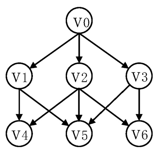
Figure 1.
Directed graph .
Definition 2
(Reverse random walk). Given vertex u in directed graph G, a reverse random walk from u is a sequence of vertices , such that is selected uniformly at random from the in-neighbors of .
Definition 3
(-walk [11]). Let c denote the decay factor, a -walk in G is defined such that (1) in each step of the reverse random walk, we have probability of stopping; (2) for the remaining probability, one of the in-neighbors of the current vertex is selected uniformly at random as the next step. We denote a -walk starting from u as , where .
According to Definition 3, Ref. [11] also defined the SimRank estimation as the total probability that -walk starting from u meets -walk starting from v, i.e., .
Definition 4
(First-meeting probability [12]). Given a reverse path -walk starting from and , the first-meeting probability of v with respect to is defined as
where is a random -walk starting from .
According to Definition 3 and 4, Ref. [12] defined as the total probability that -walk starting from u and -walk starting from v first meet at each vertex , i.e.,
Definition 5
(Shortest-meeting length). Given any two -walks starting from and starting from , and , the shortest-meeting length t between u and v is defined as the least t such that the probability of meeting after t steps is nonzero.
For example, in Figure 1, any two -walks starting from and starting from may first meet at or with walking one step, at with walking two steps. Then, the shortest-meeting length between them is 1.
Definition 6
(Approximate single-source SimRank query). In the graph , given source u, the average absolute error ε allowed in SimRank computation, and the failure probability δ, for any vertex , of an approximate single-source SimRank query returns an estimated SimRank to the ground-truth SimRank , which satisfies
Problem Statement. (Approximate single-source and top-k query) In graph , given source vertex u, decay factor c, and integer k, return the top-k vertices with the largest SimRank.
3. Related Works
In this section, we review the state-of-the-art algorithms for the single-source and top-k query problem, which are based on the widely used random walk method.
Ref. [11] first proposed the SLING algorithm, which utilizes the -walk to compute SimRank. Subsequently, several studies [9,11,14] adopted the Monte Carlo (MC) method to sample -walks for each vertex v and source u a certain number of times. By counting the number of times they meet () out of the total number of walks sampled (), the SimRank is obtained as . After computing the SimRanks with source u for all vertices and sorting them in descending order, the algorithms return the top-k results. Ref. [15] proposed the TSF algorithm based on the MC method. TSF constructs an index comprising one-way graphs that contain the coupling of random walks of length T from each vertex. This approach helps reduce storage space requirements. To address the computational cost of simulations, Ref. [16] proposed an index-based algorithm called READS. The index consists of compressed -walks, which significantly improves the efficiency of queries. In the case of MC-based algorithms, there is a problem that when the SimRank of many vertices is negligible, resulting in the -walks within a limited length not meeting the path of the source u, then the processing of these vertices is redundant. To tackle this issue, an index-free algorithm called ProbeSim was proposed by Ref. [12]. Instead of sampling -walks from each vertex v to determine whether v and source u can meet at any within the -walk from u, ProbeSim conducts a graph traversal from each to identify vertices that have a non-negligible probability of walking to . This process is repeated for iterations to obtain results with approximate guarantees. By avoiding the processing of unpromising vertices, this approach significantly reduces computational overhead. However, it requires generating a large number of probing trees to determine whether can meet every v at each step of the -walk starting from u.
To overcome the mentioned issue, Ref. [13] proposed an improved algorithm called CrashSim that builds upon the principles of ProbeSim. The main idea behind CrashSim is to consider the SimRank as the average probability of two -walks meeting within a limited length. CrashSim first computes a reverse reachable tree of source vertex u with a limited length of -walk, denoted as . It then iteratively generates a -walk for each vertex v and determines whether it can meet the limited -walk path from u with a non-negligible probability. This process is repeated for iterations to obtain approximate results with certain guarantees. By traversing the reverse reachable tree for only the source vertex u instead of exploring the entire graph for each vertex , CrashSim significantly reduces redundant computations.
However, the above mentioned algorithms require computing the SimRank for each vertex , sorting them in descending order, and returning the top-k results. Such a method results in significant redundant computational overhead when querying for a small value of k, considering that k is typically much smaller than the total number of vertices n in real-world applications.
4. HitSim
Although the state-of-the-art algorithm CrashSim reduces redundant computation by traversing the reverse reachable tree for only source vertex u, it still generates -walks for each vertex v to determine whether it can meet the -walks from u within a limited length. However, since the parameter k is typically much smaller than the total number of vertices n, processing unpromising vertices with negligible SimRank values is redundant. To overcome this issue, we propose an efficient algorithm called HitSim. It utilizes a branch and bound strategy to batch-prune unpromising vertices to avoid the redundant processing. The algorithm is implemented in three steps, as follows.
Step 1: Computing the reverse reachable tree U. In the first step of HitSim, we perform the same approach as CrashSim [13]. This involves computing the reverse reachable tree from the source vertex u and generating a matrix U. Each element in the matrix represents the probability of the -walk stopping at vertex v by walking steps.
Example 1.
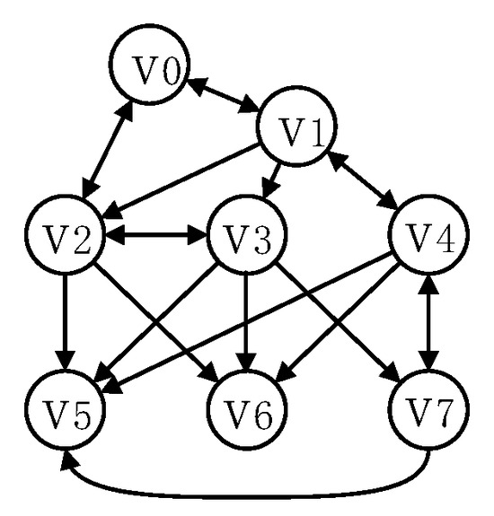
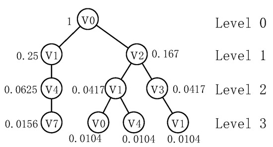
We illustrate the computation of the reverse reachable tree U using the graph shown in Figure 2. Given the source , we set the limited length of -walk to 4 and decay factor c to 0.25 (). The algorithm computes the reverse reachable tree of , which is shown in Figure 3. Note that the in-neighbor of vertex v that is equal to the parent of v is ignored to avoid recomputing the probability due to the cycle in the graph [13]. Simultaneously, it computes the probability of the -walk stopping at different vertices with different lengths. For level 0, it sets the probability . Next, for level 1, , . Similarly, for level 2, , and for level 3, .

Figure 2.
Directed graph .

Figure 3.
Reverse reachable tree of .
Step 2: Partitioning vertices. Based on CrashSim, assuming the xth sampling, if a -walk starting from v, i.e., , first meets the -walk starting from source u at , then
Lemma 1.
Given a graph and a source vertex u, if there exists a vertex , and its shortest-meeting length is , then the upper bound of SimRank for v, denoted as , is , where represents the maximum probability in level l of the reverse reachable tree of the source u.
Proof of Lemma 1.
Since the shortest-meeting length of v is , any -walk ) starting from v will not meet the -walk starting from source u before . Then, we have
Furthermore, is the maximum probability in level l of the reverse reachable tree of source u. Then,
Based on Equations (5)–(7), for any -walk ) starting from v, we have
Since , then . The average value after trials is
Thus, for any vertex v, the upper bound of SimRank is , where t is the shortest-meeting length, i.e., Lemma 1 holds. □
According to Lemma 1, for any two different vertices v and , if the shortest-meeting length of v and w are and , respectively, then and . If , then . From the above analysis, we have Observation 1 as follows:
Observation 1.
For any vertex v, the smaller the shortest-meeting length, the larger the upper bound.
According to Lemma 1, vertices with the same shortest-meeting length share the same upper bound. By partitioning the vertices into distinct sets based on their shortest-meeting lengths, we ensure that vertices within the same set share the same upper bound, i.e., for any vertex v in the same set M, , where is the upper bound of SimRank for set M. If we identify a set M satisfying , where is the minimum SimRank value of the current results, we can safely prune these unpromising vertices within M batches. According to Observation 1, we should preferentially process sets with smaller shortest-meeting lengths. Such preprocessing allows the algorithm to preferentially compute SimRank for vertices with a larger SimRank upper bound, leading to the effective pruning of unpromising vertices.
Step 3: Computing and maintaining the top-k results. Following step 2, HitSim generates -walks and computes the SimRank only for the vertices within the sets whose upper bounds exceed . Simultaneously, HitSim maintains the top-k results and the current minimum SimRank by sorting the results based on their SimRank in descending order.
Since step 1 is identical to CrashSim, we will omit its detailed description. The detailed descriptions of steps 2 (Section 4.1) and 3 (Section 4.2) are as follows.
4.1. Partitioning Vertices
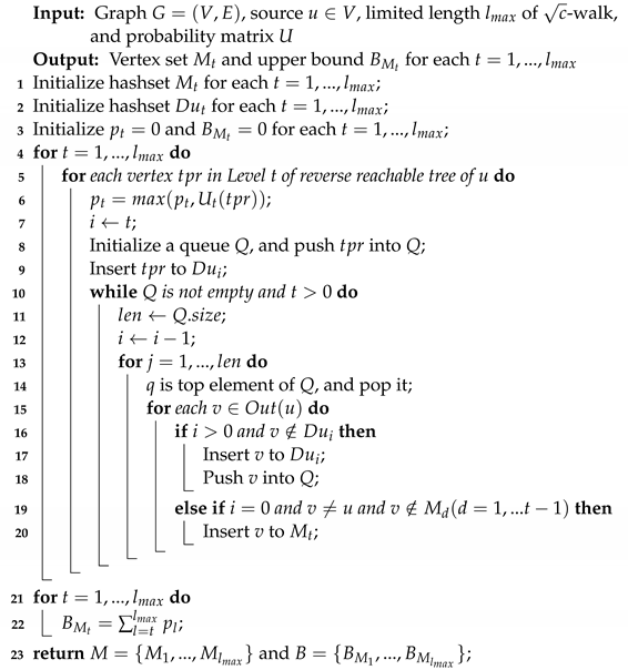
We now describe the ParVer algorithm, which is used to partition vertices into distinct sets based on their shortest-meeting lengths with the source vertex. Given a graph , a source vertex , a limited length of -walk, and a probability matrix U, ParVer returns a vertex set and the upper bound of SimRank for each , where t is the shortest-meeting length of the vertices within . Notably, does not include any vertices from the set .
The pseudo-code of ParVer is depicted in Algorithm 1. It initializes a hashset for each to store the vertices with shortest-meeting lengths equal to t (line 1). To avoid revisiting vertices of the same level, it requires a hashset for each to store the visited vertices (line 2). The probabilities and are initialized to store the maximum value of and the upper bound of SimRank of for each (line 3). To identify all the vertices within for each , it iterates over each vertex in level t of the reverse reachable tree of source u (lines 4 to 20). For each vertex in level t of the reverse reachable tree of source u, it records the current maximum probability in level t (line 6). Then, it performs forward walks of t steps from to obtain each vertex v whose shortest-meeting length is t (lines 7 to 20). Specifically, it first initializes a queue Q to store the vertices that visits in t-step forward walks. Then, it puts into Q and , where i represents the current level. Next, it forward walks from the vertex and records the size of Q. With each iteration, the step i is reduced by 1. Then, it visits Q and pops the top element q of Q. For each out-neighbor v of q, if the step of the current forward walk does not exceed the maximum walk length i and v has not been visited before, then v is inserted directly into and Q. If v does not exist in any set that stores vertices with shortest-meeting lengths from 0 to and , it is added to . Then, all the vertices within for each are obtained. Afterward, it computes the upper bound based on Lemma 1 (lines 21 to 22). Finally, ParVer returns the vertex set and its upper bound for each (line 23).
| Algorithm 1: ParVer |
 |
Example 2.
Considering the graph shown in Figure 2, we illustrate step 2, which involves the partitioning of vertices. Assume that the source vertex is . For simplicity, we set and the decay factor . In step 1, it computes the reverse reachable tree U, as shown in Example 1. Continuing from Example 1, in step 2, it partitions vertices of into distinct sets based on their shortest-meeting lengths with source . Starting with level 1 of the reverse reachable tree, it forward walks 1 step from the first vertex . Consequently, it inserts ’s out-neighbors , and into set . It omits since is the source vertex. Next, it forward walks one step from the second vertex in level 1. It inserts ’s out-neighbors and into set and omits since is already in . Thus, we have , and the maximum probability is . Moving to level 2, it forward walks 2 steps from , and , respectively. This leads to }. Note that, , and are not inserted into since they are already in . The maximum probability is computed as = 0.0625. Lastly, in level 3, it forward walks three steps from , and , respectively. As a result, , indicating that no new vertices are added to . The maximum probability is computed as . Finally, according to Lemma 1, the SimRank upper bounds of set and are computed as and , respectively.
4.2. Computing and Maintaining the Top-k Results
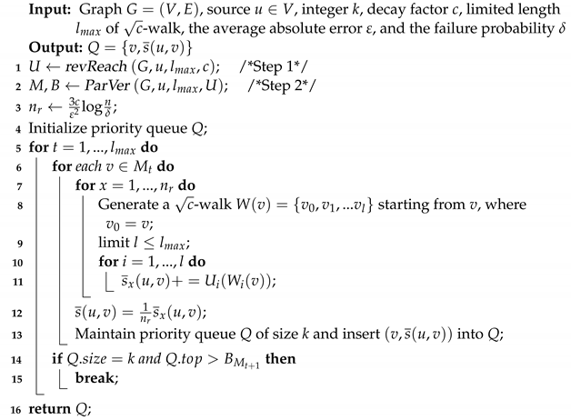
The complete pseudo-code of HitSim is illustrated in Algorithm 2. Given a graph , a source , an integer k, a decay factor c, a limited length of -walk, an average absolute error , and a failure probability , HitSim returns the queue Q of the top-k results. It first invokes the revReach algorithm (referenced as CrashSim) to construct the reverse reachable tree of source u and return a matrix U (line 1). Then, it invokes the ParVer algorithm (referenced as Algorithm 1) to partition vertices into distinct sets (line 2). Step 3, which involves computing and maintaining the top-k results, starts from line 3 of Algorithm 2.
In step 3, the algorithm initializes a priority queue Q to store the results (line 4). Based on Observation 1, for any vertex v, a smaller shortest-meeting length corresponds to a larger . Thus, HitSim processes the sets in ascending order of their shortest-meeting lengths t in order to obtain the top-k results as early as possible (lines 5 to 20). Specifically, for each vertex v in , it runs independent trials (lines 6 to 16). The computation of , which represents the minimum number of iterations that guarantees an error less than with at least , is defined by [13]. During each iteration, it generates a -walk starting from v and limits the length of the walk to (lines 8 to 9). Then, for the -walk with length i, where , it accumulates the total first-meeting probability of this walk meeting the -walk starting from u at the ith element of (lines 10 to 12). After completing the trials, it computes the average of the results to obtain the final SimRank and inserts into Q (lines 14 to 15). When the size of the current results is k, it checks whether the upper bound of the next set to be processed is larger than . If it is, HitSim continues generating -walks for the vertices within . Otherwise, it terminates and returns the current top-k results (lines 17 to 19).
| Algorithm 2: HitSim |
 |
Example 3.
Continuing from Example 2, we set k to 1; the objective of
HitSim
is to return the top-1 result. The algorithm begins by processing the first vertex within the set and . Suppose that at the xth trial, it generates a -walk starting from . It computes the SimRank as . After conducting a total of iterations, it computes the average value of . Once all the vertices in have been processed, it compares the minimum value of SimRank with the upper bound of the set . If , HitSim batch-prunes all the vertices in .
The SimRanks between and any other vertices are listed in Table 2, and they have been computed by [6] within a error. From Table 2 we can see that, due to the branch and bound strategy, HitSim is able to efficiently batch-prune vertices such as and within , whose SimRanks are notably less compared to the rest.

Table 2.
SimRank with respect to .
4.3. Analysis
The time and space complexity of HitSim can be analyzed in steps 1, 2, and 3.
- Step 1 (computing the reverse reachable tree U): In the worst case, it requires traversing each edge once and storing each vertex, resulting in a time complexity of and the space complexity is .
- Step 2 (partitioning vertices): This step involves traversing each vertex of the reverse reachable tree and storing all the vertex sets. The worst case is that we need to traverse every edge in the graph by visiting the out-neighbors of each vertex, and the worst-case time complexity is . The space complexity is .
- Step 3 (computing and maintaining the top-k results): In the worst case, it requires running trials of generating a -walk for each vertex, with a limited length of . Additionally, it requires maintaining a priority queue Q of size k. Thus, the time complexity is , and space complexity is .
In summary, the total time complexity of HitSim is , and the total space complexity is .
5. Optimization
The batch-pruning method employed in HitSim aims to prune unpromising vertices within the sets whose upper bounds of SimRank are less than the minimum SimRank of the current results. However, in certain cases, such as Example 3, where k is set to 2, the batch-pruning strategy may fail. In the example, after computing the SimRank for all vertices in , the current top-2 results are and , with a minimum SimRank of approximately 0.074, as shown in Table 2. Comparing with the upper bound , HitSim continues to compute the SimRank for vertices and within , indicating a failure of the batch-pruning method.
The reason for this failure is that in dense graphs, vertices may have a large number of in-neighbors. Vertices with the same shortest-meeting length but significantly different SimRanks can be partitioned into the same set, leading to imprecise pruning. For instance, in , the reverse reachable tree of (shown in Figure 4) reveals that cannot meet source at in level 2, where is the maximum value in level 2. Similarly, cannot meet source at in level 3, where is the maximum value in level 3. Consequently, although is partitioned into , its upper bound , computed by accumulating the maximum values from level 2 and level 3, significantly exceeds its actual upper bound . When processing such sets (e.g., ), it becomes inevitable to compute the SimRank for the vertices with a small SimRank (e.g., ), leading to the batch pruning being ineffective.
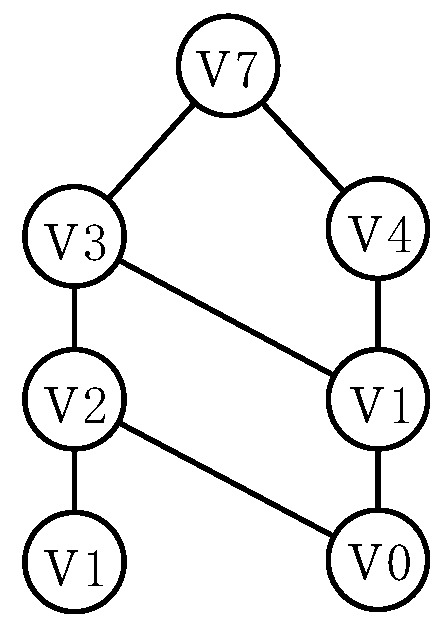
Figure 4.
Reverse reachable tree of .
To address the issue, we propose an optimized algorithm called HitSim-OPT. HitSim-OPT aims to perform fine-grained and effective vertex pruning by computing a tighter upper bound of SimRank for each individual vertex, instead of that for each set. The optimized algorithm consists of the following three steps.
Step 1: Computing the reverse reachable tree U. The details of this step are omitted as they are the same as step 1 of HitSim.
Step 2: Computing the upper bound of SimRank for each vertex. According to Lemma 1, the upper bound of SimRank for any vertex v is computed by , where t represents the shortest-meeting length and denotes the maximum probability in level l of the reverse reachable tree of u. To refine the upper bound , we introduce a modification by replacing with , which represents the maximum probability in level l of the reverse tree of v. Since each vertex in the reverse reachable tree of v is the potential vertex within the -walks starting from v, provides a more precise bounding than .
By utilizing the inequality , we can ensure . Consequently, we can carefully modify the upper bound for each vertex v as
Step 3: Maintaining the top-k results. Similar to step 3 of HitSim, HitSim-OPT maintains the top-k results and the current minimum SimRank by sorting the results based on their SimRank in descending order. For each vertex v, HitSim-OPT determines whether to further compute its actual SimRank by comparing with . If is less than , HitSim-OPT prunes v.
Since step 1 is identical to that of HitSim, we will omit its detailed description. The detailed descriptions of the algorithms in steps 2 (Section 5.1) and 3 (Section 5.2) are as follows.
5.1. Computing Upper Bound of SimRank for Each Vertex
A straightforward approach is to construct a reverse reachable tree for each vertex v and compute the maximum probability of v meeting the source vertex u at each level of u’s reverse reachable tree, as computed by Equation (10). Taking from Figure 2 as an example, we construct the reverse reachable tree of , as shown in Figure 4. At level 1, the maximum probability is 0 because cannot meet the source vertex with one step (see the reverse reachable tree of source in Figure 3). In level 2, the maximum probability is 0.0417 as can meet at with two steps. Similarly, in level 3, the maximum probability is 0.0104 as can meet at either or with three steps. By accumulating the maximum probabilities of the three levels, we obtain .
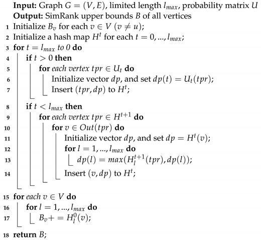
However, constructing a reverse reachable tree for each vertex in the straightforward approach suffers from significant challenges in terms of time and space complexity. To address this challenge, we further propose a more efficient method called UBV (Upper Bound of Vertex) based on dynamic programming to compute the upper bound of SimRank for each vertex v. It utilizes an array of length for each potential meeting point w to store the maximum probabilities at levels 0 to . Such processing allows the algorithm to only traverse source u’s reverse reachable tree once instead of constructing a reverse reachable tree for each vertex. For each potential meeting point w in level , represents the maximum probability that v can meet u at level i. UBV dynamically computes for each w starting from the bottom of u’s reverse reachable tree. By the end of the traversal of level 0, a set of values can be obtained, where the vertices w in level 0 are those that can meet u within steps. The upper bounds of SimRank for these vertices are computed as .
Lemma 2.
For each potential meeting point w, the state array in level t is computed by the following equation.
where is the probability of source u traversing and stopping at vertex w, and is the in-neighbor of vertex w.
Proof of Lemma 2.
(1) When , the -walk starting from w at level t cannot meet any vertex at level i in the reverse reachable tree of source vertex u, thus ; (2) When , the -walk starting from w at level t happens to meet w itself, thus ; (3) When , the -walk starting from w at level t must pass through one of its in-neighbors, denoted as . In this case, is equal to the maximum probability among its in-neighbors meeting at level i, i.e., . □
The pseudo-code of UBV is illustrated in Algorithm 3. UBV initializes an array for each in the reverse reachable tree of source vertex u from the bottom to the top (lines 4 to 9). Subsequently, it updates for each out-neighbor of based on Equation (11) (lines 10 to 20). Note that the vertices v at level 0 represent the vertices that can meet u within steps, and denotes the upper bounds of SimRank (lines 22 to 26).
| Algorithm 3: UBV |
 |
Example 4.
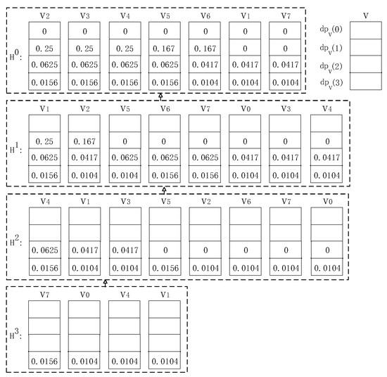
We use in Figure 2 to illustrate step 2 ofHitSim-OPT, i.e., the computation of the SimRank upper bound for each vertex. Given source , for simplicity, we set and the decay factor . Continuing with Example 2,HitSim-OPTcomputes the upper bound of SimRank for each vertex. Specifically,UBVinitializes a hash map for each level t to store the array’s . Starting from the bottom of u’s reverse reachable tree, it sets , and based on Equation (11). After the first iteration , the result is shown in Figure 5. When ,UBVfirst sets , , and . Then,UBVcomputes for all the out-neighbors of each . After this iteration, is obtained. Similarly, when and 0, and can be obtained. Finally,UBVcomputes for each . The upper bounds of all vertices are .

Figure 5.
Array of each vertex.
5.2. Maintaining the Top-k Results
To obtain the top-k results, the algorithm requires computing SimRank for vertices whose upper bounds of SimRank are larger than the current minimum SimRank . However, the computation of SimRank involves a large number of iterations for generating -walks to obtain an average value. Ref. [13] defines the minimum number of iterations, denoted as , that guarantees an error less than with at least . However, when increases, the number of iterations for generating -walks also increases. This can lead to significant time consumption when computing SimRank for the vertices with negligible SimRank. Here, we introduce an effective method to avoid the redundant generation for such vertices. Based on Lemma 3, at the xth iteration, we assume that the SimRanks of the remaining iterations are all computed as the upper bound , if the average value of total iterations is not larger than the current minimum SimRank ; then, we can safely skip the computation of the remaining iterations and prune this vertex. This enables us to reduce computational overhead and improve efficiency.
Lemma 3.
During the computation of SimRank for vertex v, at the xth iteration for generating a -walk, if
then the remaining iterations can be safely skipped.
Proof of Lemma 3.
Since is the upper bound of the SimRank of v, for any yth trial, we have
Furthermore,
Then, we have
The complete pseudo-code of HitSim-OPT is illustrated in Algorithm 4. It first invokes the revReach algorithm (referenced as CrashSim [13]) to construct the reverse reachable tree of source u and return a matrix U (line 1). Subsequently, it invokes the UBV algorithm to compute the upper bound for each vertex v (line 2).
| Algorithm 4: HitSim-OPT |
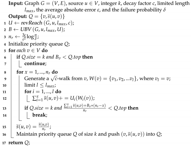 |
In step 3, it maintains a priority queue Q of size k to store the top-k results (lines 4 to 22). Specifically, it determines whether to prune v to avoid generating -walks for v by comparing with the top element in Q. If , v can be pruned (lines 6 to 8). If v is not pruned, the algorithm generates a -walk for trials to compute for v (lines 9 to 20). During the trials, if the current satisfies Lemma 3, the generation process breaks (lines 15 to 17).
5.3. Analysis
The time and space complexity of HitSim-OPT can be analyzed in steps 1, 2, and 3.
- Step 1 (computing the reverse reachable tree U). It is the same as step 1 of HitSim.
- Step 2 (computing the upper bound of SimRank for each vertex). Computing an array of for all vertices is essential, resulting in a time complexity of and a space complexity of .
- Step 3 (maintaining the top-k results). It is the same as step 3 of HitSim.
Based on the above analysis, the total time complexity of HitSim-OPT is , and space complexity is .
6. Experiments
6.1. Experimental Setup
We conduct extensive experiments to evaluate the performance of our algorithms. The algorithms evaluated in our experiments are summarized as follows:
- MC [14];
- CrashSim [13];
- HitSim: Algorithm 2;
- HitSim-OPT: Algorithm 4.
We conduct all the experiments on an Ubuntu machine with Intel(R) Core(TM) i7-12700 CPU 2.10 GHz and 64 G memory. All of the algorithms are implemented in C++.
Datasets. We used six datasets to evaluate the performance of all the algorithms. The dataset soc-Epinions (http://konect.cc/networks/ (accessed on 20 September 2022)) represents the trust network from the online social network Epinions; emai-EuAll (http://snap.stanford.edu/data/ (accessed on 1 December 2021)) is the email communication network of a large European institution; amazon (http://konect.cc/networks/ (accessed on 20 September 2022)) is the network of items on Amazon; wiki-topcats (http://snap.stanford.edu/data/ (accessed on 1 December 2021)) is a web graph of Wikipedia hyperlinks; soc-LiveJournal (http://snap.stanford.edu/data/ (accessed on 1 December 2021)) is a free online community with almost 10 million members; wikipedia-link-en (http://konect.cc/networks/ (accessed on 20 September 2022)) consists of the wikilinks of Wikipedia in the English language. These datasets represent relevant knowledge in various fields. Detailed statistics of these datasets are summarized in Table 3, where , , and denote the number of vertices, the number of edges, and the average of degrees.

Table 3.
Statistics of datasets.
Parameters. Consistent with previous studies [3,7,13,17], we set the decay factor c to 0.6 and to 5. To evaluate the performance under different error guarantees, we vary the parameter to achieve overall absolute error guarantees of 0.1, 0.05, 0.025, and 0.0125, while maintaining a failure probability of .
Metrics. For evaluating the quality of results for each single-source and top-k query from the source vertex u, we employ two metrics: and . The metric, representing the average absolute error, is computed as , where is the true SimRank score between vertices u and v, and is the SimRank estimation. The metric measures the proportion of correctly identified results among the top-k results. It is computed as , where represents the list of top-k vertices returned by the algorithm being evaluated, and represents the ground-truth top-k results.
6.2. Performance of Algorithms
Absolute error in querying (AE@50). In this experiment, we set k to 50 and vary from 0.1 to 0.05, 0.025, and 0.0125. Figure 6 illustrates the trade-offs between and the query time of each algorithm. We can observe that as decreases the value of decreases. However, the query time increases for each algorithm. The curves in the graph show a near-linear relationship, suggesting that the algorithms achieve a faster query time when is large.
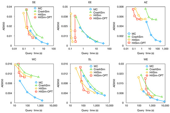
Figure 6.
The performance of .
Additionally, when comparing algorithms with the same parameters, both HitSim and HitSim-OPT demonstrate similar average values compared to CrashSim, while requiring less query time. This can be attributed to the fact that CrashSim computes SimRank for all vertices to obtain the top-k results, whereas HitSim only computes SimRank for vertices within sets whose upper bounds of SimRank exceed , and HitSim-OPT computes SimRank only for vertices with larger upper bounds.
It is worth noting that the results of MC may be unstable when (the number of iterations) is not sufficiently large, as MC requires generating a large number of -walks for each vertex v to determine if it meets source u.
Precision in querying (Precision@50). In this experiment, we fix the value of k to 50 and vary the parameter from 0.1 to 0.05, 0.025, and 0.0125. The trade-off between and query time is illustrated in Figure 7. We observe that, as decreases, both and the query time increase. When , all algorithms achieve a precision of nearly 1. The curves in the graph show a near-linear relationship, indicating that algorithms achieve a faster query time when is large.
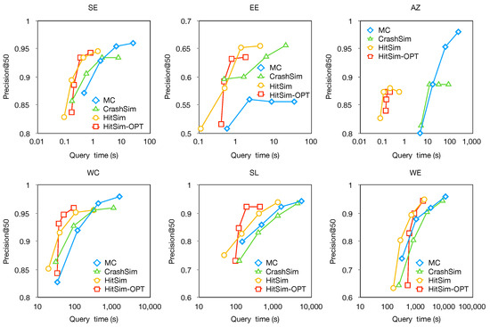
Figure 7.
The performance of .
Moreover, when comparing algorithms with the same parameters, both HitSim and HitSim-OPT demonstrate similar precision values compared to CrashSim, while requiring less query time. The reason is the same as the last experiment. The results of MC may be unstable when (the number of iterations) is not sufficiently large.
Running time. In this experiment, we compare the running time of querying the top-250 results using the same parameters for each algorithm. Figure 8 shows the running time of each algorithm. The results demonstrate that on all datasets HitSim and HitSim-OPT exhibit faster performance compared to MC and CrashSim. Specifically, HitSim is approximately 7 times faster than MC on average and 3 times faster than CrashSim. Similarly, HitSim-OPT is approximately 30 times faster than MC on average and 11 times faster than CrashSim.
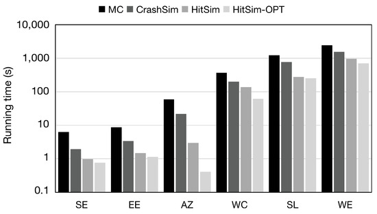
Figure 8.
Running time of top-250 results query under the same parameters.
The main reason is that CrashSim processes all vertices, whereas HitSim only processes the vertices within sets whose upper bounds of SimRank exceed , and HitSim-OPT processes only vertices with larger upper bounds. As mentioned in the previous analysis, the running time of generating -walks for vertices dominates the overall performance. Therefore, processing fewer vertices results in less time cost for HitSim and HitSim-OPT compared to MC and CrashSim.
To validate the correctness, we also test the number of vertices processed by each algorithm, as shown in Table 4. The results confirm that MC and CrashSim process all the vertices, while HitSim and HitSim-OPT process significantly fewer vertices due to their batch-pruning methods. Additionally, the number of vertices processed by MC or CrashSim is approximately 4 times more than HitSim on average and 16 times more than HitSim-OPT. The results demonstrate that HitSim and HitSim-OPT can efficiently return the single-source and top-k query.

Table 4.
The number of vertices processed. The column total represents the total number of vertices processed by HitSim-OPT, while the column iteration represents the number of vertices that completed all iterations of -walks.
Performance of HitSim and HitSim-OPT. In this experiment, we compare the performance of the preprocessing and query steps of HitSim and HitSim-OPT under the parameters and . As described in Section 4, HitSim and HitSim-OPT return the top-k results in three steps. We consider the first two steps as preprocessing and the third step as the query phase.
Figure 9 illustrates the performance comparison between the preprocessing and query steps of HitSim and HitSim-OPT on all datasets. The results indicate that Hitsim-OPT outperforms HitSim. Notably, the preprocessing step of HitSim-OPT is slower than that of HitSim. This is attributed to the fact that HitSim-OPT requires constructing arrays of length for all vertices on the reverse reachable tree to obtain their SimRank upper bounds, whereas HitSim only requires visiting all vertices on the reverse reachable tree. The query performance of HitSim-OPT demonstrates a significant improvement over HitSim. This enhancement can be attributed to the finer-grained pruning rules of HitSim-OPT, allowing it to achieve efficiency by processing fewer vertices. However, in large-scale dense graphs such as SL and WE, many vertices’ upper bounds may be quite similar, resulting in a large number of vertices meeting the processing condition (upper bound ). Nonetheless, during the processing phase, HitSim-OPT leverages its efficient pruning rule (Lemma 3) to early-terminate -walks, which is the most time-consuming operation. As a result, many vertices do not need to complete all the iterations of -walks, thereby reducing the computational overhead. For instance, on SL, only 597 vertices complete all iterations of -walks, while 3,841,961 − 597 = 3,841,364 vertices execute 1 to iterations of -walks. Similarly, on WE, only 849 vertices complete all iterations of -walks, while 5,147,351 − 849 = 5,146,502 vertices execute 1 to iterations of -walks.
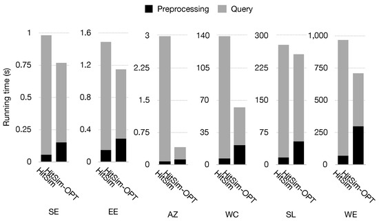
Figure 9.
Preprocessing and query of HitSim and Hitsim-OPT.
Scalability. In this experiment, we test the scalability of HitSim and HitSim-OPT. We generate four subgraphs by randomly sampling 20–80% of the edges from the WE dataset. We test the running time of HitSim and HitSim-OPT on WE with fixed parameters , and . Figure 10 shows the results of the scalability test. We can see that both HitSim and HitSim-OPT show near-scalability as the number of edges increases from 20% to 100%, and as the value of k ranges from 20 to 2000. Additionally, we note that as k increases, the running time of both HitSim and HitSim-OPT also increases. This is because the batch-pruning strategy is triggered later as k increases.
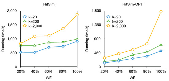
Figure 10.
Scalability tests of HitSim and HitSim-OPT by varying from 20% to 100% and k from 20 to 2000 on WE.
7. Conclusions
In this paper, we study the single-source and top-k SimRank query problem. We first propose an efficient algorithm called HitSim that utilizes a branch-and-bound strategy. HitSim partitions vertices into distinct sets based on their shortest-meeting lengths to the source vertex. Subsequently, it computes the upper bound of SimRank for each set. By batch-pruning vertices within the same set whose upper bound is less than the minimum SimRank of the current results, HitSim significantly enhances computational efficiency. Furthermore, we propose an optimized algorithm called HitSim-OPT, which employs a fine-grained pruning strategy. HitSim-OPT computes the upper bound of SimRank for each vertex, thereby improving pruning efficiency. Our experimental results on six real-world datasets demonstrate that, while maintaining comparable precision and absolute error to CrashSim, HitSim achieves an average speedup of 3 times compared to CrashSim, and HitSim-OPT achieves an average speedup of 11 times.
Author Contributions
Conceptualization, J.B. and J.Z.; methodology, J.B. and M.M.; software, M.M. and S.C.; validation, J.B. and J.Z.; formal analysis, M.D. and M.M.; investigation, J.B., M.M. and S.C.; data curation, J.B.; writing—original draft preparation, M.M. and J.B.; writing—review and editing, J.B. and J.Z.; supervision, J.Z., M.D. and Z.C.; funding acquisition, J.Z. All authors have read and agreed to the published version of the manuscript.
Funding
This research was funded by grants from the Natural Science Foundation of China (No.: 62372101, 61873337, 62272097).
Institutional Review Board Statement
Not applicable.
Informed Consent Statement
Not applicable.
Data Availability Statement
The data that support the findings of this study are available on request from the first author upon reasonable request.
Conflicts of Interest
The authors declare no conflicts of interest.
References
- Jin, R.; Lee, V.E.; Hong, H. Axiomatic ranking of network role similarity. In Proceedings of the 17th ACM SIGKDD International Conference on Knowledge Discovery and Data Mining, San Diego, CA, USA, 21–24 August 2011; pp. 922–930. [Google Scholar] [CrossRef]
- Liben-Nowell, D.; Kleinberg, J.M. The link-prediction problem for social networks. J. Assoc. Inf. Sci. Technol. 2007, 58, 1019–1031. [Google Scholar] [CrossRef]
- Antonellis, I.; Garcia-Molina, H.; Chang, C. Simrank++: Query rewriting through link analysis of the click graph. Proc. VLDB Endow. 2008, 1, 408–421. [Google Scholar] [CrossRef]
- Spirin, N.; Han, J. Survey on web spam detection: Principles and algorithms. SIGKDD Explor. 2011, 13, 50–64. [Google Scholar] [CrossRef]
- Rothe, S.; Schütze, H. CoSimRank: A Flexible & Efficient Graph-Theoretic Similarity Measure. In Proceedings of the 52nd Annual Meeting of the Association for Computational Linguistics, ACL 2014, Baltimore, MD, USA, 22–27 June 2014;: Long Papers; Volume 1, pp. 1392–1402. [Google Scholar] [CrossRef]
- Jeh, G.; Widom, J. SimRank: A measure of structural-context similarity. In Proceedings of the Eighth ACM SIGKDD International Conference on Knowledge Discovery and Data Mining, Edmonton, AB, Canada, 23–26 July 2002; pp. 538–543. [Google Scholar] [CrossRef]
- Lizorkin, D.; Velikhov, P.E.; Grinev, M.N.; Turdakov, D. Accuracy estimate and optimization techniques for SimRank computation. VLDB J. 2010, 19, 45–66. [Google Scholar] [CrossRef]
- Tao, W.; Yu, M.; Li, G. Efficient Top-K SimRank-based Similarity Join. Proc. VLDB Endow. 2014, 8, 317–328. [Google Scholar] [CrossRef]
- Fogaras, D.; Rácz, B. Scaling link-based similarity search. In Proceedings of the 14th International Conference on World Wide Web, WWW 2005, Chiba, Japan, 10–14 May 2005; pp. 641–650. [Google Scholar] [CrossRef]
- Lee, P.; Lakshmanan, L.V.S.; Yu, J.X. On Top-k Structural Similarity Search. In Proceedings of the IEEE 28th International Conference on Data Engineering (ICDE 2012), Washington, DC, USA, 1–5 April 2012; pp. 774–785. [Google Scholar] [CrossRef]
- Tian, B.; Xiao, X. SLING: A Near-Optimal Index Structure for SimRank. In Proceedings of the 2016 International Conference on Management of Data, SIGMOD Conference 2016, San Francisco, CA, USA, 26 June–1 July 2016; pp. 1859–1874. [Google Scholar] [CrossRef]
- Liu, Y.; Zheng, B.; He, X.; Wei, Z.; Xiao, X.; Zheng, K.; Lu, J. ProbeSim: Scalable Single-Source and Top-k SimRank Computations on Dynamic Graphs. Proc. VLDB Endow. 2017, 11, 14–26. [Google Scholar] [CrossRef]
- Li, M.; Choudhury, F.M.; Borovica-Gajic, R.; Wang, Z.; Xin, J.; Li, J. CrashSim: An Efficient Algorithm for Computing SimRank over Static and Temporal Graphs. In Proceedings of the 36th IEEE International Conference on Data Engineering, ICDE 2020, Dallas, TX, USA, 20–24 April 2020; pp. 1141–1152. [Google Scholar] [CrossRef]
- Liu, Y.; Zou, L.; Ge, Q.; Wei, Z. SimTab: Accuracy-Guaranteed SimRank Queries through Tighter Confidence Bounds and Multi-Armed Bandits. Proc. VLDB Endow. 2020, 13, 2202–2214. [Google Scholar] [CrossRef]
- Shao, Y.; Cui, B.; Chen, L.; Liu, M.; Xie, X. An Efficient Similarity Search Framework for SimRank over Large Dynamic Graphs. Proc. VLDB Endow. 2015, 8, 838–849. [Google Scholar] [CrossRef]
- Jiang, M.; Fu, A.W.; Wong, R.C.; Wang, K. READS: A Random Walk Approach for Efficient and Accurate Dynamic SimRank. Proc. VLDB Endow. 2017, 10, 937–948. [Google Scholar] [CrossRef]
- Wei, Z.; He, X.; Xiao, X.; Wang, S.; Liu, Y.; Du, X.; Wen, J. PRSim: Sublinear Time SimRank Computation on Large Power-Law Graphs. In Proceedings of the 2019 International Conference on Management of Data, SIGMOD Conference 2019, Amsterdam, The Netherlands, 30 June–5 July 2019; pp. 1042–1059. [Google Scholar] [CrossRef]
Disclaimer/Publisher’s Note: The statements, opinions and data contained in all publications are solely those of the individual author(s) and contributor(s) and not of MDPI and/or the editor(s). MDPI and/or the editor(s) disclaim responsibility for any injury to people or property resulting from any ideas, methods, instructions or products referred to in the content. |
© 2024 by the authors. Licensee MDPI, Basel, Switzerland. This article is an open access article distributed under the terms and conditions of the Creative Commons Attribution (CC BY) license (https://creativecommons.org/licenses/by/4.0/).