Abstract
Rationale. Object tracking has significance in many applications ranging from control of unmanned vehicles to autonomous monitoring of specific situations and events, especially when providing safety for patients with certain adverse conditions such as epileptic seizures. Conventional tracking methods face many challenges, such as the need for dedicated attached devices or tags, influence by high image noise, complex object movements, and intensive computational requirements. We have developed earlier computationally efficient algorithms for global optical flow reconstruction of group velocities that provide means for convulsive seizure detection and have potential applications in fall and apnea detection. Here, we address the challenge of using the same calculated group velocities for object tracking in parallel. Methods. We propose a novel optical flow-based method for object tracking. It utilizes real-time image sequences from the camera and directly reconstructs global motion-group parameters of the content. These parameters can steer a rectangular region of interest surrounding the moving object to follow the target. The method successfully applies to multi-spectral data, further improving its effectiveness. Besides serving as a modular extension to clinical alerting applications, the novel technique, compared with other available approaches, may provide real-time computational advantages as well as improved stability to noisy inputs. Results. Experimental results on simulated tests and complex real-world data demonstrate the method’s capabilities. The proposed optical flow reconstruction can provide accurate, robust, and faster results compared to current state-of-the-art approaches.
1. Introduction
The method presented in the current paper addresses medical applications where the strategic goal is to provide better medical care through real-time detection, warning, prevention, diagnosis, and treatment. The specific task is to detect seizures in people who have epilepsy.
Epilepsy is a neurological disease whose symptoms are sudden transitions from normal to pathological behavioral states called epileptic seizures, often accompanied by rhythmic movements of body parts. Some of these seizures may lead to life-threatening conditions and ultimately cause Sudden Unexplained Death in Epilepsy (SUDEP).
Therefore, medical treatment involves continuous observation of individuals for long periods to obtain sufficient data for an adequate diagnosis and to plan therapeutic strategies. Some people, especially those with untreatable epileptic conditions, may need long-term care in specialist units to allow early intervention that prevents complications.
We have developed and implemented an earlier method that detects motor seizures in real time using remote optical sensing by video camera. Human video surveillance is used successfully for monitoring patients, but it poses certain societal burdens and costs and creates ethical issues related to privacy. Epilepsy patients are sick people who are often stigmatized and sensitive to privacy issues. Therefore, it is necessary to use only remote sensing devices (i.e., no contact with the subject) such as video cameras and automated video processing.
The method was published [1], and its modification is currently used in medical facilities with validated detection success. It uses a spectral modification of the classical optical flow algorithms with an original, efficient algorithm (GLORIA) to reconstruct global optical flow group velocities. These quantities also provide input for detecting falls and non-obstructive apnea [2,3]. However, the technique only works in static situations, for example, during night observations when the patient lies in bed. When the patient changes position, for example, during daytime observation, the operator has to adjust either the camera’s field of view with PTZ (pen-tilt zoom) or the region of interest (ROI). Here, we address the challenge of developing and embedding patient-tracking functionality in our system. We approach this task using the same group velocities provided by the GLORIA algorithm. This way, we avoid introducing extra computational complexity that may prevent the system from being used in real-time. To the best of our knowledge, this is a novel video-tracking approach and constitutes the main contribution of this work. Below, we acknowledge other works related to video tracking, but none of them can directly utilize the group velocities that also provide input for our convulsive seizure detection algorithm.
Real-time automated tracking of moving objects is a technique with a wide range of applications in various research and commercial fields [4]. Examples include self-driving cars [5,6], automated surveillance for incident detection and criminal activity [7], traffic flow control [8,9], interfaces for human–computer interactions and inputs [10,11,12], and patient care, including intensive care unit monitoring and epileptic seizure alerts [1,13].
Generally, there are different requirements and limitations when one attempts to track a moving object, such as noise in the video data, complex object movement, occlusions, illumination changes between frames, and processing complexity. Many object-tracking methods involve particular tracking strategies [14,15,16,17], including frame difference methods [18], background subtraction [19], image segmentation, static and deep learning algorithms [20,21], and optic flow methods. All the methods have advantages and disadvantages, and the choice depends on the specific task.
In the current work, we propose a method based on direct global motion parameter reconstruction from optical camera frame sequences. As noted above, the main reason for focusing on such a method is that it uses already calculated quantities as part of the convulsive seizure detection system. This method avoids intensive pixel-level optic flow calculation and thus provides computationally efficient and content-independent tracking capabilities. Tracking methods that use the standard pixel-based optic flow reconstruction [22,23] suffer from limitations caused by relatively high computational costs and ambiguities due to the absence of sufficient variation of the luminance in the frames. We propose a solution to these limitations using the multi-spectral direct group parameter reconstruction algorithm GLORIA, developed by our group and introduced in [24]. The GLORIA algorithm offers the following advantages compared to other optic flow-based tracking techniques: (A) It directly calculates the rates of group transformations (such as, but not limited to, translations, rotation, dilatation, and shear) of the whole scene. Thus, it avoids calculating the velocity vector fields for each image point, lowering computational requirements. (B) Unlike the standard intensity-based algorithms, we apply a multi-channel method directly using co-registered data from various sources, such as multi-spectral and thermal cameras. This early fusion of sensory data features increases accuracy and decreases possible ambiguities of the optic flow inverse problem.
Our objective for the particular application here is to track a single object that moves within the camera’s field of view. We introduce a rectangular region of interest (ROI with a specific size around the object we plan to track). This GLORIA method then further accurately estimates how the object moves. Subsequently, the novel algorithm proposed here adjusts the ROI accordingly. Using an ROI also helps reduce the size of the images for optical flow estimation and limits the adverse effects of any areas with high levels of brightness change outside the ROI. It also automatically disregards movements of no interest to us outside the specified area. In short, our approach reduces the tracking problem to a dynamic ROI steering algorithm.
The present work is part of a more extensive study on autonomous video surveillance of epilepsy patients. Tracking how a patient moves can further improve results related to seizure detection from video data [1]. The proposed method, however, is not limited to use only in health care but can successfully apply to other scenarios related to automated remote tracking. The term “remote” here (as well as throughout the rest of this paper) relates to “remote sensing” and is used to indicate that the optical sensor (camera) used for object tracking is positioned remotely (i.e., not attached to the object of interest).
The rest of the paper is organized as follows. The next section introduces the proposed original tracking method. Then, we present our results from both simulated and real-world image sequences. We also apply the novel method to a sequence from a publicly available dataset (LaSoT). The outcome from all the examples provides quantitative validation of the algorithm’s effectiveness and qualitative illustrations. Finally, in the Discussion section, we comment on the features, possible extensions, and limitations of the proposed approach to tracking.
2. Methods
2.1. Optic Flow Reconstruction Problem
The algorithm presented in the current work uses motion information reconstructed from the optic flow in video sequences. Optical flow reconstruction is a general technique that enables determining the spatial velocities of a vector field from changes in luminance spectral intensities between sequential observed scenes (frames). Here, we briefly introduce optic flow methods, leaving the details to the dedicated literature [25,26,27,28,29,30,31,32,33].
We denote the pixel content in a multi-spectral image frame as , where are the spatial coordinates and the time, and is the spectral index, most commonly labeling the R, G, and B channels. Assuming that all changes in the image content in time are due to scene deformation and defining the local vector velocity (rates of deformation) vector field as , the corresponding image transformation is:
In Equation (1), is the vector field operator, are the two-dimensional spatial coordinates in each frame, and is the time or frame number. The velocity field can determine a large variety of object motion properties such as translations, rotations, dilatations (expansions and contractions), etc. In the current work, however, we do not need to calculate the velocity vector field for each point, as we can directly reconstruct global features of the optic flow, considering only specific aggregated values associated with it. In particular, we are interested in the global two-dimensional linear non-homogeneous transformations consisting of translations, rotations, dilatations, and shear transformations. Therefore, we use the Global Optical-flow Reconstruction Iterative Algorithm “GLORIA”, which was developed previously by our group [3]. The vector field operator introduced in Equation (1) takes the following form:
The Equation (2) representation can be helpful when decomposing the transformation field as a superposition of known transformations. If we denote the vector fields corresponding to each transformation generator within a group as , and the corresponding parameters as , then:
With Equation (3) one may define a set of differential operators for the group of transformations that form a Lie algebra:
As a particular case, we apply Equation (4) to the group of three general linear non-homogeneous transformations in two-dimensional images that preserve the orientation of the axes and the ratio between their lengths:
Here, denotes the commutator between two operators. The last two lines of Equation (5) give the commutation relations between the group generators that form a Lie algebra.
In particular, the action of the group described by Equation (5) on the spatial coordinates is ).
It is obvious that the above transformation preserves the aspect ratio and orientation of the image axes. This property of the generating Lie algebra is important for the specific target applications, as discussed in the next section.
2.2. Region of Interest (ROI) Transformations
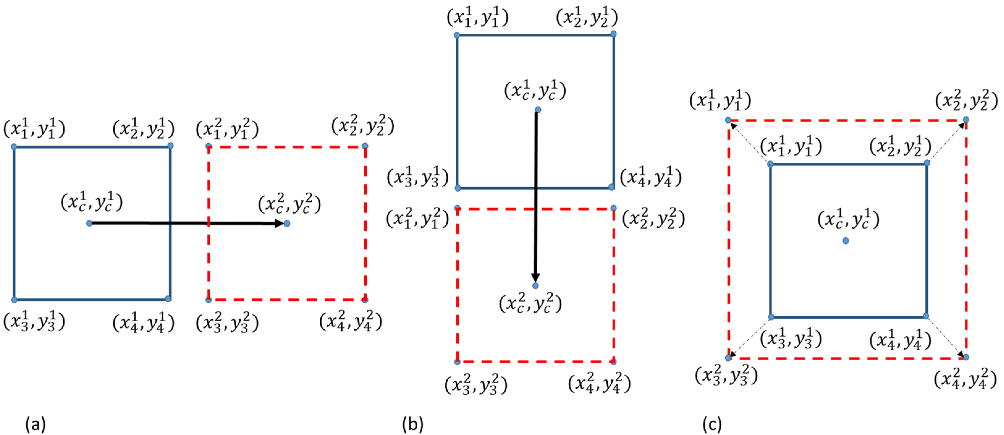
Using GLORIA, the amplitudes for each of the three transformation vector fields are the solution to the global transformation optic flow inverse problem. These amplitudes represent the rate of each type of movement as defined by Equation (4). These amplitudes, along with the coordinates of the initial region R1 of interest (corner and center points), can be used to determine iteratively the coordinates of the subsequent region of interest R2. Figure 1 illustrates the changes in ROI due to the impact of each group transformation.
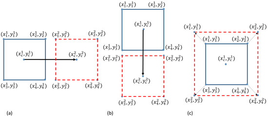
Figure 1.
ROI evolution, based on the values of the global transformation parameters. The figure shows the three elementary motions of the points of the ROI—corner points for ; center coordinates of the ROI . (a) Translation along the x-axis. (b) Translation along the y-axis. (c) Dilatation or “scaling” of the ROI.
The movement of an object can be followed using the values of the group transformations reconstructed from the GLORIA algorithm by updating the ROI after each (or a set number of) frame(s). The general process can be summarized in the following steps: initial region of interest selection, calculation of global motion parameters for each two consecutive frames, and update of the ROI’s position based on the calculation results.
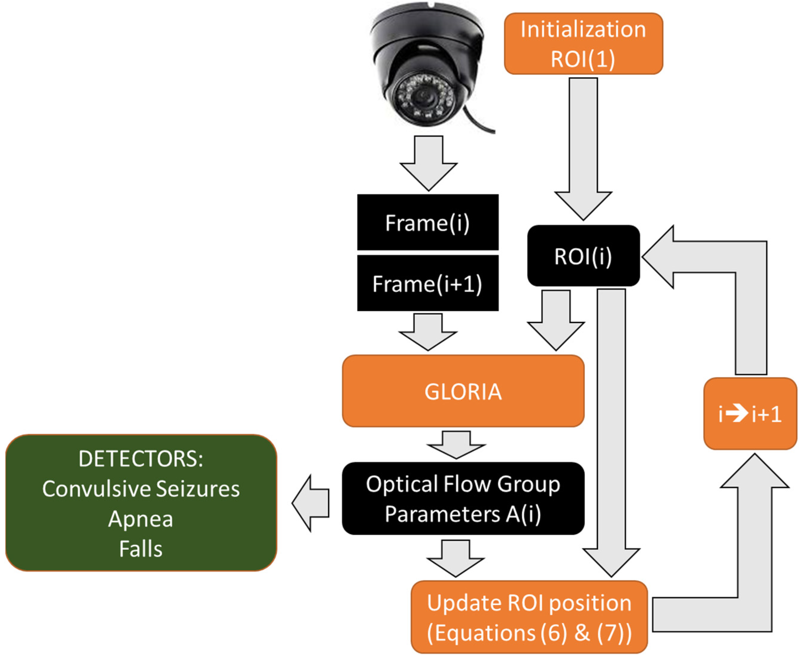
The diagram presented in Figure 2 outlines the entire tracking process. A camera is used to acquire the video feed. Objects of interest in the field of view are singled out through ROI selection (or PTZ control of the camera). Optic flow information from their specific movement is acquired and used to update the ROI iteratively for each subsequent pair of video frames, realizing the tracking of a person or an object of interest. The tracking algorithm is specifically designed to be lightweight so that it can run in parallel with detectors in a medical (or patient monitoring) setting, such as epileptic seizure detection, apnea detection, and more. This can be computationally efficient as such detectors also rely on optic flow analysis. While we note that the sharing of optic flow information for the simultaneous running of multiple patient monitoring detectors is a possible future direction, such discussion goes beyond the scope of the present work.

Figure 2.
Diagram of the tracking process. The black boxes represent data, and the orange ones the processing steps. The initial region of interest (RoI) is specified in the first frame by an operator. Following the selection of center coordinates and size of the RoI, global motion parameters are calculated for each two consecutive frames, and the RoI is updated for the next frame based on the calculation results. The calculated optical flow group transformation rates can then be used to track a person’s movement. This method can run in parallel, serving as a pre-processing module, to various detectors, such as the ones enlisted in the green box.
The method in this work can be applied to any group of transformations. Our choice here is on the two translation rates and the dilatation (a global scale factor quantity) that are provided by the first three generators from Equation (5). We mark them as and for the translations and for the dilatation, where indicates which two consecutive frames were used for the calculation. We restrict the current method to only these three transformations because we do not intend to rotate the ROI with the tracked object nor change the ratio between the ROI dimensions. In this way, our method is directly applicable to a situation where pan, tilt, and zoom (PTZ) hardware actuators are affecting the camera field of view that corresponds to the two translations (pen and tilt) and the dilatation (the zoom). Next, we define the values that will parametrize the extent of our ROI. These values, related to the rectangular ROI in Figure 3, are its width and length .
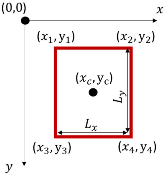
Figure 3.
Coordinates and size of rectangular ROI. The center point of the ROI has coordinates while the corner points are marked as for i = 1–4.
They relate to the corner points of the ROI by Equation (6):
The first step of our algorithm then becomes the selection of the coordinates of the center ) and the width and length of a region of interest R1 from the initial frame in the video sequence or live feed.
Using the same region of interest in the next frame, we calculate the global rates of translation and the dilatation D1 by applying the GLORIA algorithm between the two frames. The center and sizes of the subsequent region of interest R2 are then defined by the elements of the initial frame, and the values are calculated by GLORIA according to the following set of equations:
Equation (7) allows us to track an object by adjusting the ROI containing the object with each following frame. In particular, if a PTZ steerable camera is used, the changes in the ROI’s center coordinates in the and direction would require pan and tilt actions to re-center the scene, and changes in the ROI’s size due to the dilatation would translate into a zoom-in or zoom-out action. This process is repeated for all subsequent frames, updating the ROI’s elements along the way.
2.3. Evaluation of the ROI Tracking Performance
We introduce several quantities to assess the proposed method’s accuracy and working boundaries. The first one reflects a combination of the absolute difference between the center coordinates of the moving object and the calculated values of the center coordinates of the ROI, as well as the absolute differences between the true and calculated values of the dimensions of the ROI:
We use these values to determine the maximum velocities of moving objects that can be registered with the method. They only apply when the ROI’s ground truth coordinates and sizes are known, for example, when dealing with synthetic test data. To assess the average deviation between the true position of the moving object and the detected one for a given tracking sequence, we define the following quantity:
In Equation (9), is the total number of frames, and the values in brackets are the summed values of Equation (8) for the corresponding number of frames. Equation (9) represents the average values of Equation (8) for frames. We apply the measure in Equation (9) to explore the influence of the background image contrast on the accuracy of our tracking algorithm. Image contrast is defined, following [34], as the root-mean-square deviation of the pixel intensity from the mean pixel intensity for the whole frame, divided by the mean pixel intensity for the entire frame. Each color channel has a specific background contrast value. It can affect the optical flow reconstruction quality and, accordingly, the quality of the ROI tracking.
Initial ROI placement also affects the accuracy of the method. To determine the optimal size of the initial ROI, we define the ratio between the ROI area and object area Equation (10):
If one wants to verify that the ROI tracks the object accurately but does not have access to the true ROI center position dimensions (as in Equation (8)), we introduce the relative mismatch :
In Equation (11), is the image in the ROI in the frame, resampled to the pixel size of the initial ROI, is the initial image from the initial ROI in the first frame, is the index of the current frame, and is a summation index over all the pixels of and . In our tests, we will show that the quantities and are highly correlated using two correlation measures—the Pearson correlation coefficient and the nonlinear association index , developed in [35]. This would mean one might use the relative mismatch to give a qualitative measure of the accuracy of the method in real-world data where the true positions and sizes of moving objects are unknown.
The precision value is a measure used in the literature for tracking performance evaluation. It is defined as the ratio between the number of frames in which the center location is below some threshold and the total number of frames in the sequence:
Another measure is the success rate, which also considers the ROI box’s size and compares it to ground truth. It is defined as the relative number of frames where the area of intersection between the tracked ROI with the ground truth bounding box divided by the area of the union between the two is larger than some threshold
Here, is the intersection-over-union between the tracking region of interest of the frame and the ground truth region of interest. The function is an indicator which returns a value of “1” if is above the current threshold , and “0” otherwise.
We note the last two quantifiers of tracking quality, like the ones defined by Equations (8) and (9), depend on the existence of “unequivocal” ground truth. For a general assessment of tracking quality, the quantity introduced by Equation (11) applies to complex objects and scenes.
3. Results
3.1. Tracking Capabilities
To show the feasibility of our method, we started by creating simple simulated test cases with only a single moving object. Initially, we made tests of movements comprised of only one of the primary generators in Equation (5). The test methodology goes as follows:
- Generate an initial image, in our case, a Gaussian spot with a starting size and coordinates on a homogenous background;
- Specify the coordinates and size of the first region of interest, R1;
- Transform the initial image with any number of basic movement generators, as described in Figure 1, to arrive at an image sequence;
- Using the GLORIA algorithm, calculate the transformation parameters;
- Update the ROI according to Equation (7);
- Compare properties of regions of interest—coordinates and size.
3.2. Tests with Simulated Data
For translations in only the or direction, the method proved to be very effective.
Figure 4a shows the Gaussian “blob” moving horizontally with a speed of two pixels per frame to the right in the first row, while in the second row, the object’s velocity is one pixel per frame, vertically. Figure 4b shows how much the calculated values deviated from the original. Although there is some spread, the final region of interest selection uses integer values for pixel coordinates, meaning that those computed values are rounded up. After rounding the values calculated by GLORIA and applying Equations (8) and (11), both and show a positive linear correlation with a Pearson coefficient value of 1. Therefore, the complete positive linear correlation between the two measures of tracking precision shows that can be used instead of for translational motion tracking assessment.
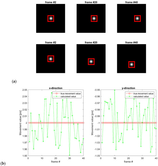
Figure 4.
(a) Demonstration of ROI tracking in the case of translational movement. The top row displays an example of translational movement in the x-direction. The moving object is a Gaussian “blob” at different moments in time—frames #2, #20, and #40. Similarly, the bottom row shows the translational movement of a Gaussian blob in the y-direction. The selected moments in time are again at frames #2, #20, and #40. The rectangular region of interest successfully follows the moving object in both tests. (b) Comparison between the calculated and actual values of the moving objects depending on the current frame. Red circular markers show the actual movement values, while green star markers show the calculated values. The maximum deviations are ±0.05 pixels per frame change, less than 5% for the y-direction and 2.5% for the x-direction. The ROI that tracks the object is displayed in red.
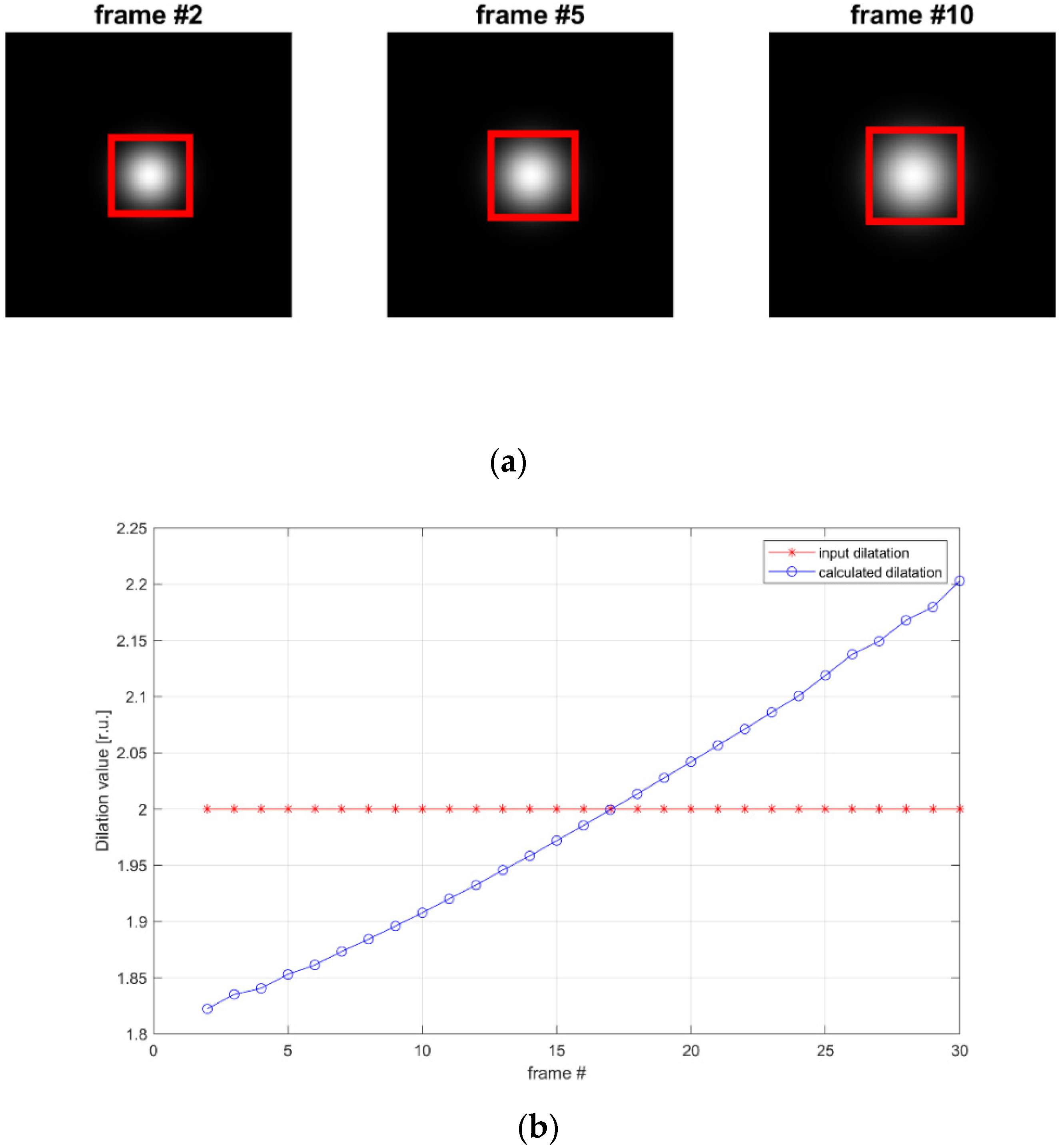
Further, we demonstrate the usefulness of the GLORIA algorithm when estimating the dilatational transformation rate (see Figure 5). In this test, the size of the observed object is increased by a fixed amount with each frame. The algorithm successfully detected the scaling of the object.
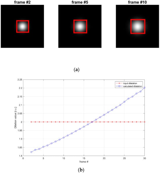
Figure 5.
Scaling of an object and its detection. (a) An object-gaussian “blob” is increasing, and the corresponding ROI tracks those changes. The object is displayed in specific moments in time—frames #2, #5, and #10. (b) Comparison between the calculated and actual values of the object depending on the current frame. Some differences in the range of 10% of the reconstructed parameter can be observed. The ROI that tracks the object is displayed in red.
The mismatch values and are calculated again. However, this time, they only exhibit a partial linear correlation. We provide their scatter plot in Figure 6.
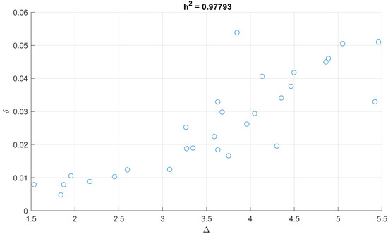
Figure 6.
Scatter plot of values and for the tests with tracking scaling (dilatation). The h2 nonlinear association index value is provided in the title.
The nonlinear association index h2 value shows that and have a high nonlinear correlation. The variance of values obtained by Equation (8) can be explained by the variance of values obtained by Equation (11) for dilatational movements.
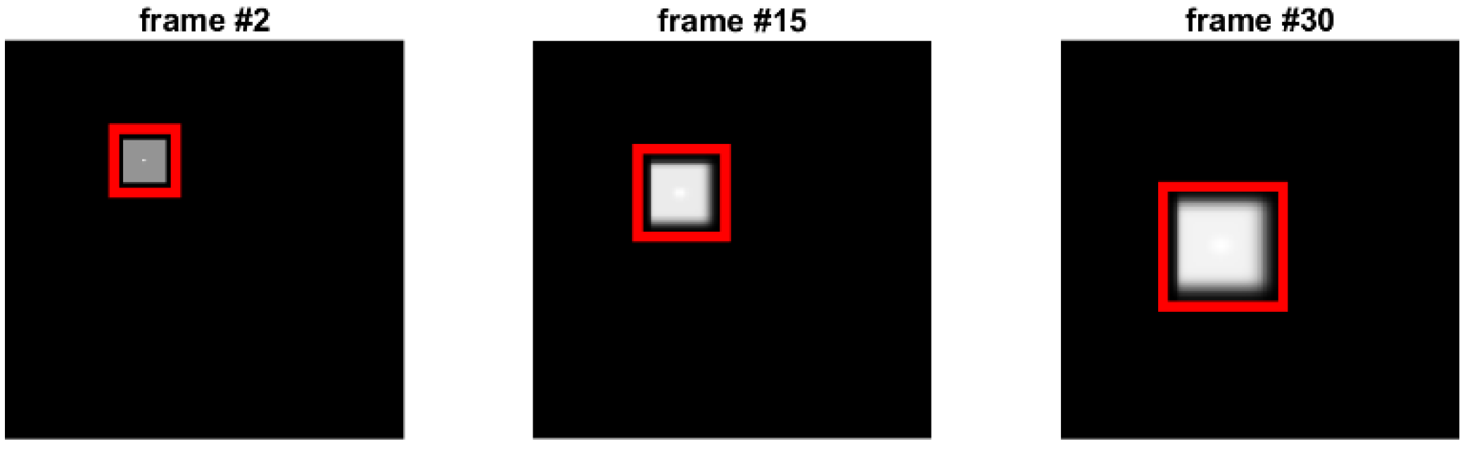
The next step is to show the tracking capabilities of our method when multiple types of movement are involved, as illustrated in Figure 7. We have prepared a test where both translations and dilatation are present.
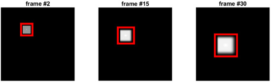
Figure 7.
A test with translational and dilatational movements present. Here, the moving object is a rectangle. It is shown in different moments in time—frames #2, #15, and #30. The object moves simultaneously to the left and downwards while increasing in size. The tracking ROI is shown in red.
We applied both Equations (8) and (11) to this test to show that both measures are highly correlated, and the relative mismatch can be used for cases where no ground truth is available. The linear correlation between the measures and is much lower than the nonlinear association index which accounts for arbitrary functional relations. The measured between the two mismatch measures , and is 0.8103. In other words, the variance of the values given by Equation (8) can be explained by the variance of the values given by Equation (11), and this fact, alongside the results from Figure 4 and Figure 6, allows using the relative mismatch for real-world data.
3.3. Influence of the Background
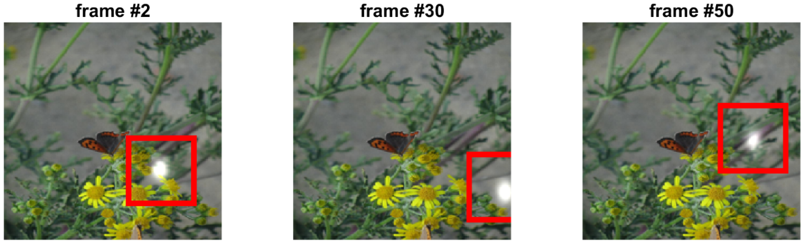
In Figure 8, we combined different types of movement and changed the scene’s background. We tested both low-contrast and high-contrast backgrounds. Our method works both with grayscale and RGB data.

Figure 8.
Tracking a moving object on a complex RGB background. The object is a Gaussian “blob” shown in different moments in time—frames #2, #30, and #50. The ROI that tracks the object is displayed in red.
3.4. Tests with Real-World Data
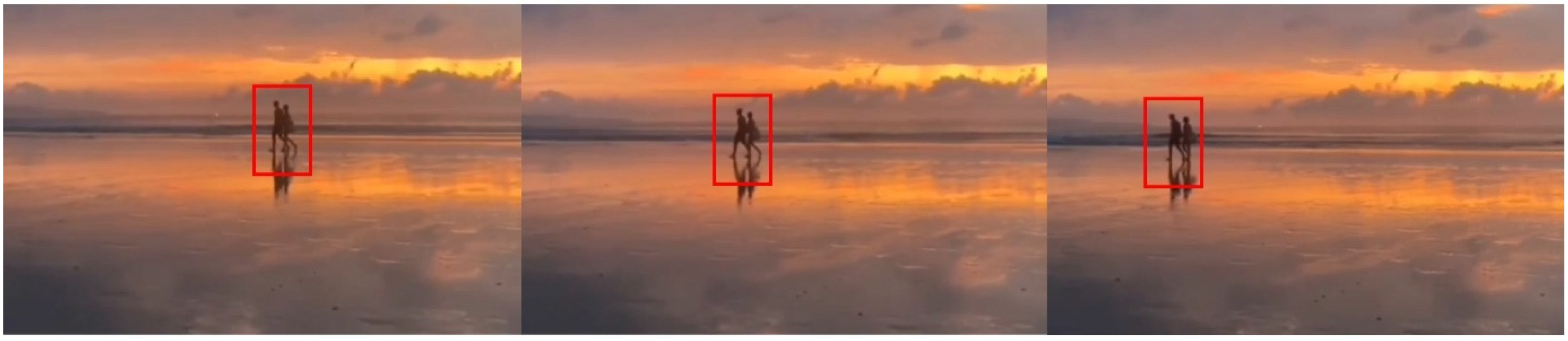
After the initial tests, we tried applying it to various real-world tracking scenarios, which showed accurate tracking results as well. We started with a video sequence that contained only one moving party to track with a relatively static background (see Figure 9). The method successfully estimated a proper region of interest around the moving objects.

Figure 9.
Tracking in a real-world scenario. A video of a couple walking on a beach. The background is static. The ROI tracking the moving people is shown in red.
Finally, we tested a dynamic scene (see Figure 10) with multiple moving objects and a high-contrast background.
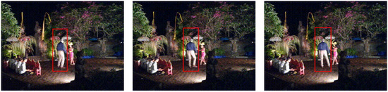
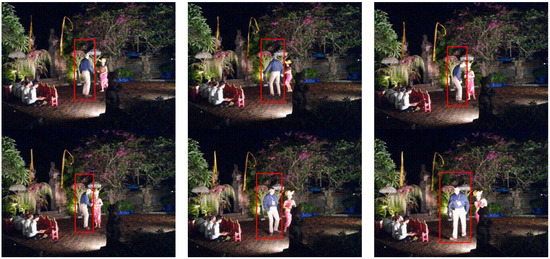
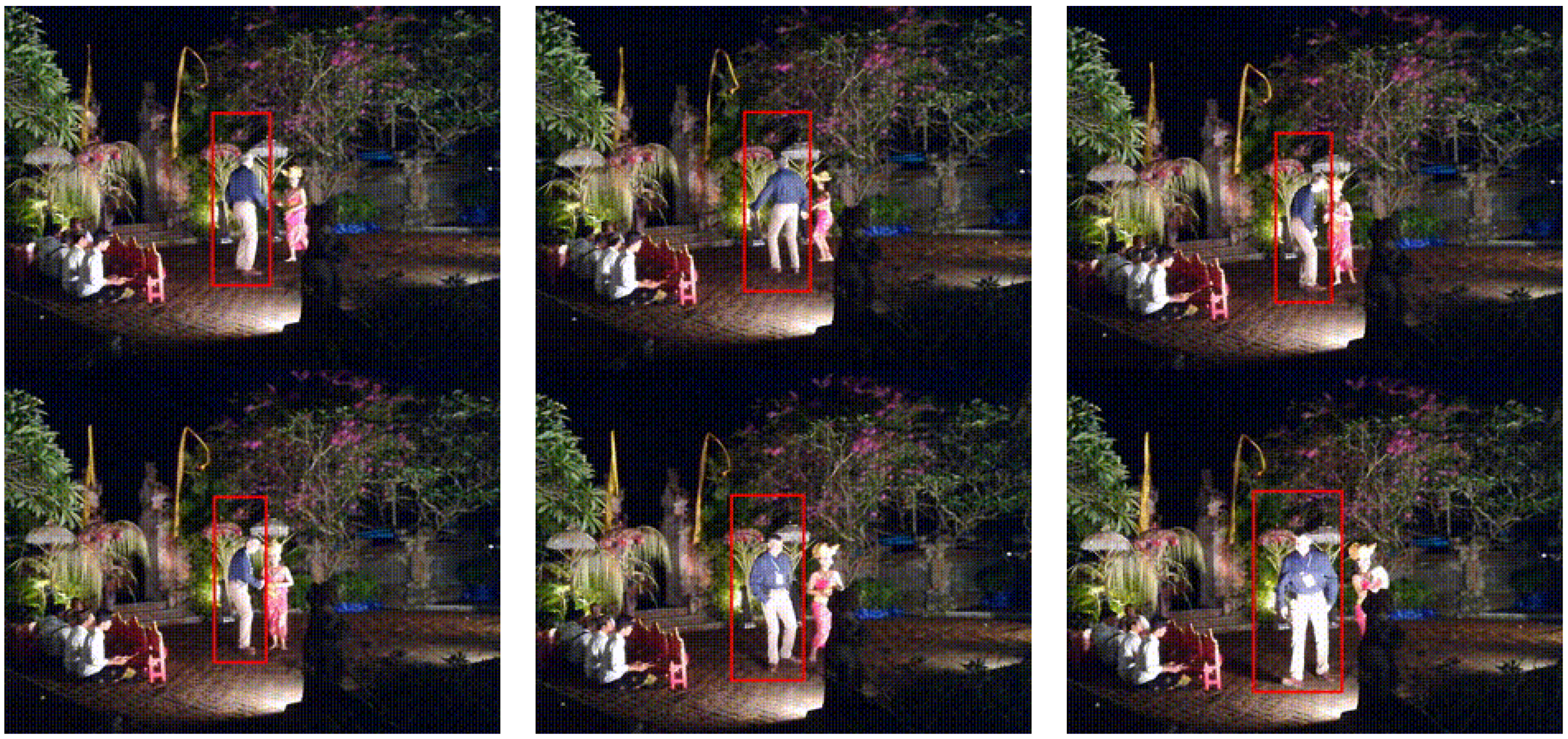
Figure 10.
Tracking a dancing man. Nine frames from the video are provided, with frame order from top to bottom and from left to right. The background is dynamic, with other moving objects in the frame. The ROI is shown in red.
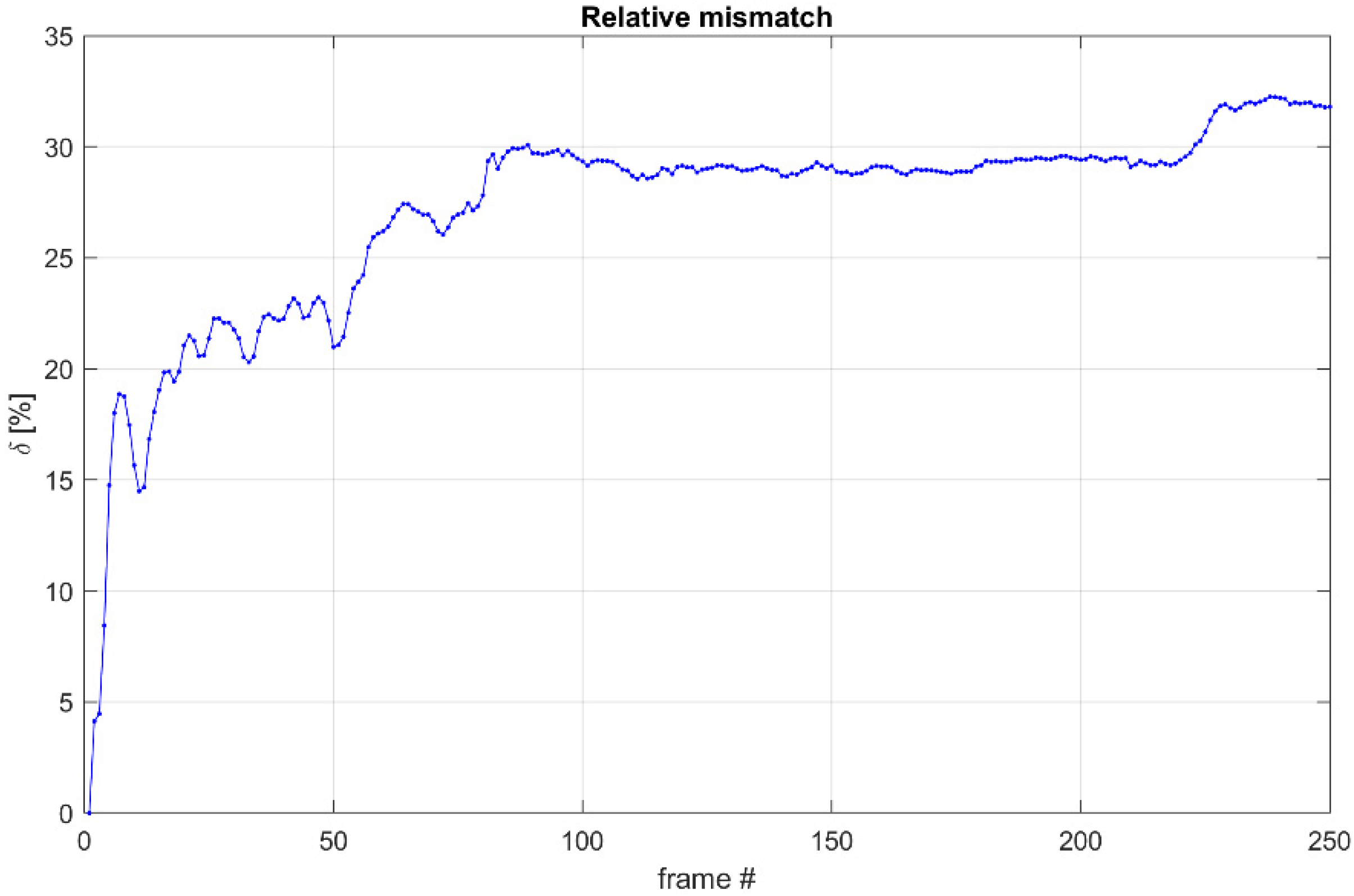
The results in Figure 10 show the benefits of the proposed method. It can easily track the person in the ROI throughout the frames. Although the background is complex and there are other moving objects, the ROI stays centered around the man and changes size accordingly based on the distance to the camera (which can be observed in the last presented frame). The relative mismatch for the video sequence in Figure 10 is shown in Figure 11.
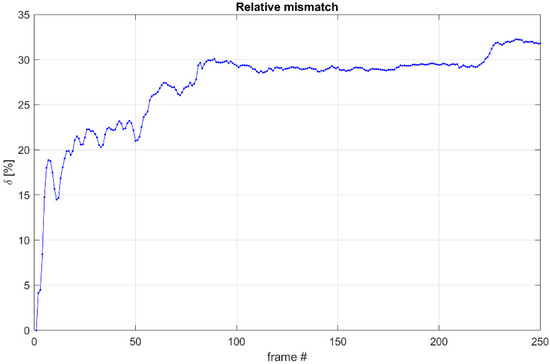
Figure 11.
Relative mismatch throughout the different frames from the video sequence. The mean value for is 27% for all 250 frames. The y-axis shows the value of , while the x-axis shows the frame number.
3.5. Tests on the Public Database LaSOT
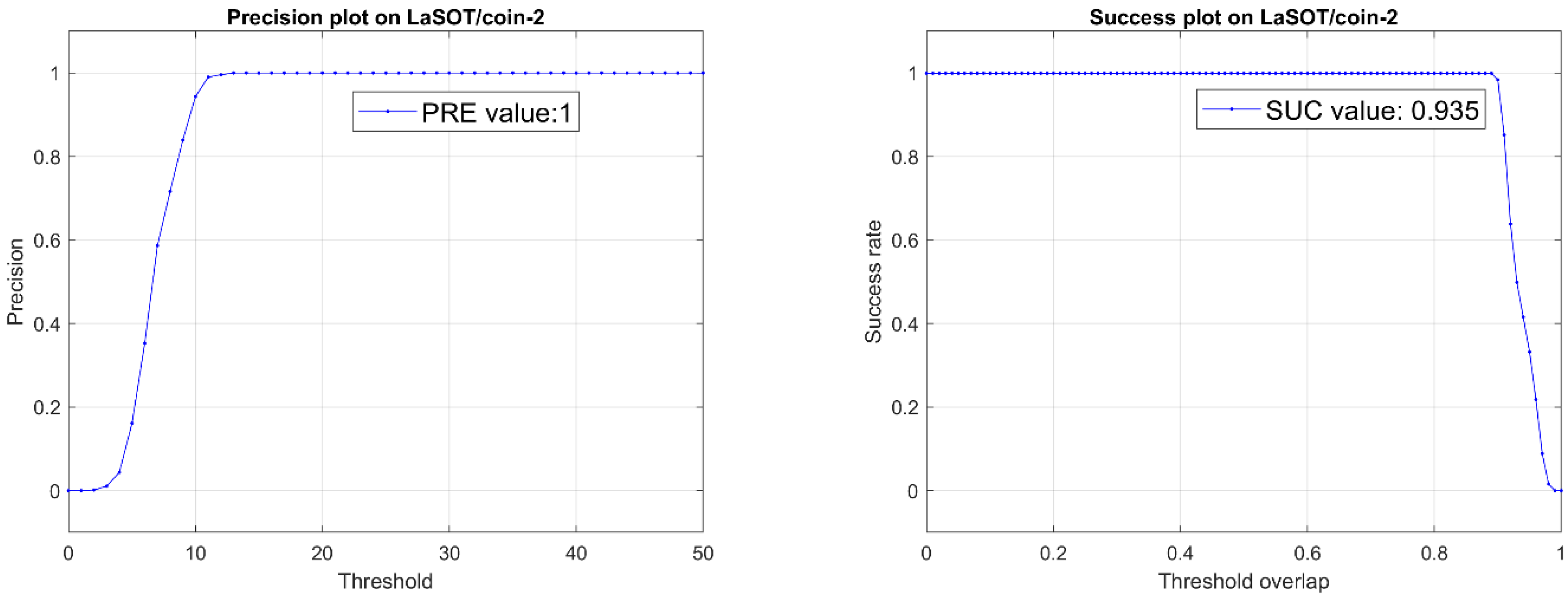
To test the performance of our method with test data provided for the evaluation of tracking methods [20], we have applied it to a sample of image sequences from the LaSOT dataset [36]. We provide the precision (Equation (12)) and success (Equation (13)) plots in Figure 12. The initial ROI for our method is the same as the RoI from the first image in the specific LaSOT image sequence.
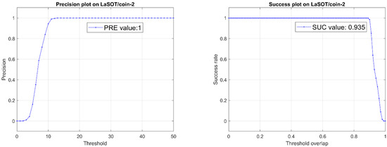
Figure 12.
The precision graph (left) and success graph (right) on the coin-2 image sequence from the LaSOT dataset. The PRE value displayed in the legend in the left frame is the precision at a threshold of 20 pixels. The SUC value in the plot legend to the right is the area under the success curve. Both PRE = 1 and SUC = 0.935 values are very high compared to other methods tested on the LaSOT database. Again, we note that the values in the figure are for the specific coin-2 example.
The achieved processing speeds are 14 FPS on the CPU and 63 FPS on the GPU for an ROI with a size of 550 × 550 pix2. More information on computational time speed is available in the following section on tracking limitations. Our method shows higher precision and success values in this example than the dataset’s averaged performance of any of the other tested methods [34]. This is certainly not a conclusive comparison, but it still indicates that the proposed technique provides promising tracking abilities. Comparisons such as these may not be adequate due to the differences in scope and requirements specific to the relevant use cases. The intended specific application of the current method is the real-time tracking of patients. In this context, the use of machine learning methods can be problematic, as they require a significant amount of data for model training. Such information is very sensitive due to ethical and privacy considerations. Our method uses the video feed to extract relevant optic flow data (in the form of three global motion parameters) and uses it to update the position of a region of interest. No patient video data needs to be stored. Other differences include the contents of the public video datasets—they are not representative of the conditions and specifics of the patient tracking task. It is also worth noting that in the context of patient monitoring, it is beneficial for a tracking algorithm to be parallelizable. This way, the algorithm may run smoothly alongside detection or alarming algorithms.
3.6. Multi-Spectral vs. Mono-Spectral Results
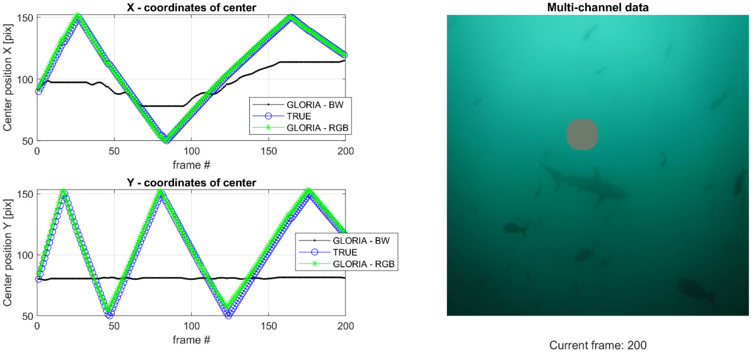
Our method works significantly better when multi-spectral data are used. This is a consequence of the GLORIA algorithm, which provides an early fusion of all spectral components and reduces any contrast-related ambiguities for the group parameter reconstruction. We have prepared an example demonstrating the importance of multi-channel data (in our case, the use of colored image sequences). The test is presented in Figure 13. We have prepared a moving object (circle) on a shallow contrast background image. The moving object is not trackable in greyscale but is successfully tracked when the video has all three color channels.

Figure 13.
On the left side: true (blue circle markers) and measured (green star markers for RGB data, black dot markers for greyscale (BW) data) positions of the center of the moving object. The current frame is displayed on the x-axis. The top graph displays the X-coordinate of the object’s center, while the bottom graph displays the Y-coordinate of the object’s center. The measured positions acquired from colored videos overlap almost entirely with the actual positions of the object. On the right side is a snapshot from the video of the moving circle; the background is low in contrast.
3.7. Tracking Limitations
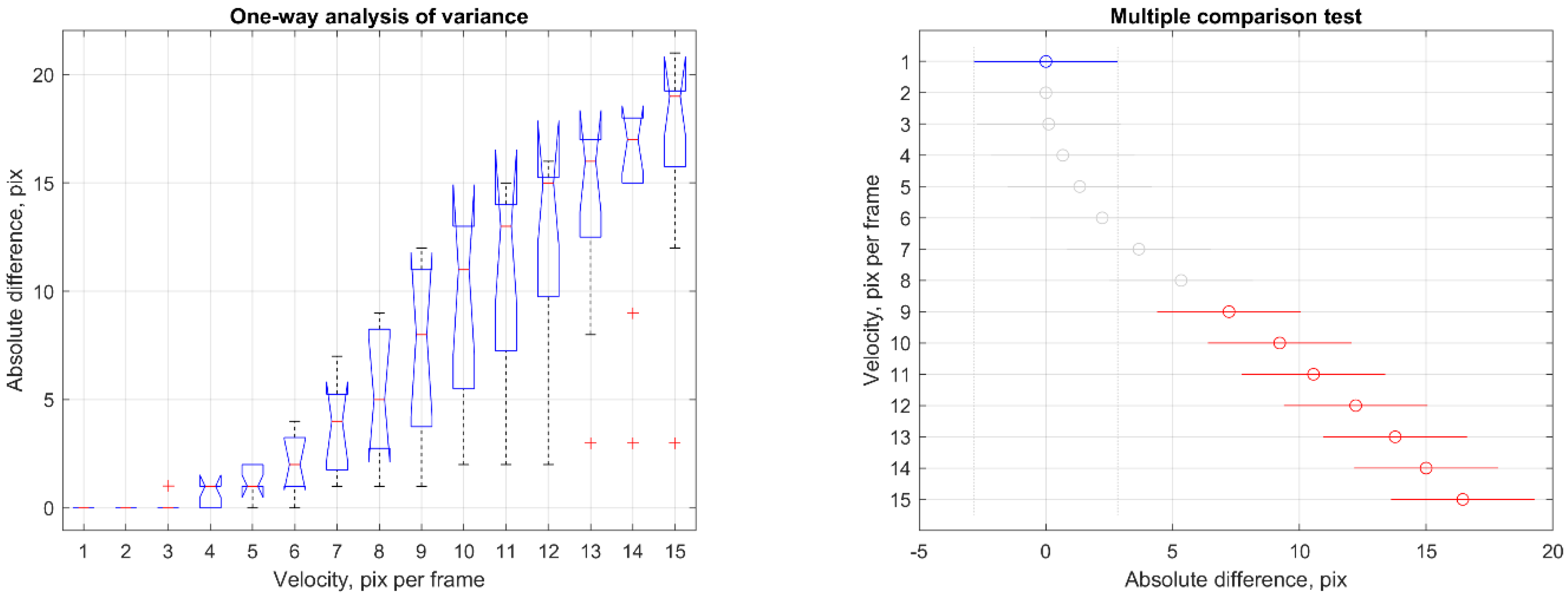
Several limitations apply when using the method presented in the current work. One is the maximum speed with which an object can move and be tracked by our method. To find the extent of this limitation, we made numerous simulations of a moving circular spot on a homogenous background with varying speeds. We use Equation (8) to compare the method’s accuracy for varying object velocities. The means of the quantities of Equation (8) were analyzed for movement spread out in twenty consecutive positions (frames), and a one-way analysis of variances test can summarize the results (see Figure 14).
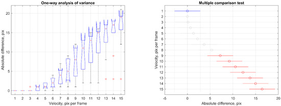
Figure 14.
Analysis of variance (left) and multiple comparison tests (right) for maximum velocity estimation. The velocity in pixels per frame is given on the x-axis of the ANOVA graph (left). In contrast, the medians and variances of the absolute differences are provided on the y-axis. Outliers are marked with a plus sign, while the dotted lines, or whiskers, indicate the most extreme data points which are not outliers. The red central mark indicates the median on each box, while the edges are the 25th and 75th percentiles. On the multiple comparison test to the right, the blue, grey and red bars represent the first velocity’s comparison interval, and the circle marker indicates the mean value.
The tests show that the tracking method becomes less reliable for velocities over seven pixels per frame, and some inaccuracies become apparent.
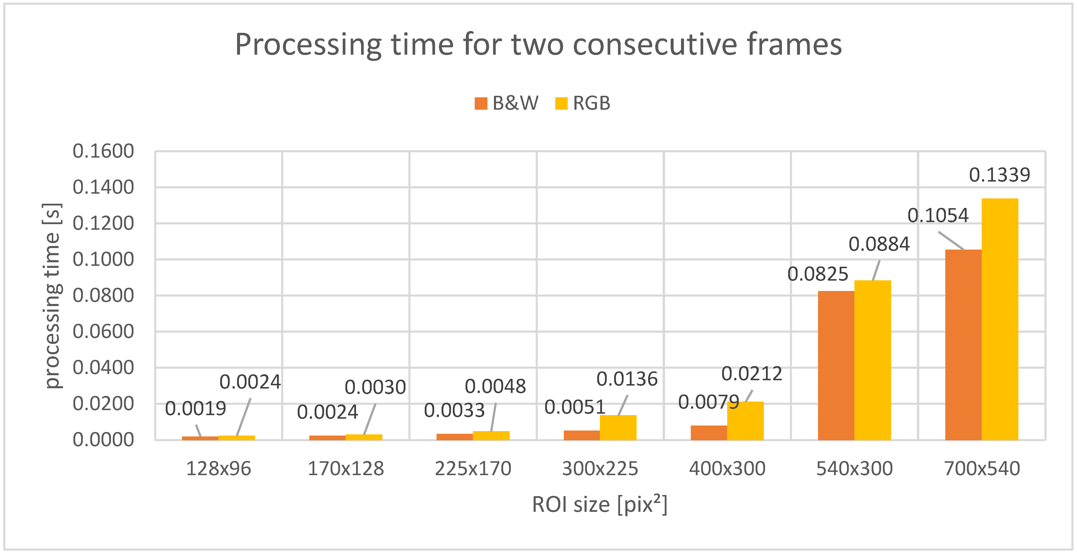
Another critical detail of our method is its applicability in real-time image sequences. It is limited by the processing time needed to update the ROI between frames. We investigated how fast our algorithm is on a personal computer with an Intel® Core™ i9-10909x CPU, 32 GB of RAM, and an NVIDIA® GeForce GTX1060 SUPER GPU. Results for processing time depending on ROI size are presented in Figure 15.
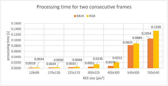
Figure 15.
Analysis of CPU processing times. The y-axis shows processing times, while the x-axis shows the size in squared pixels of the tracked ROI. Both RGB and B&W tests are shown.
The graph shows that real-time calculations between each frame can be performed for a smaller ROI. However, our initial tests with a PTZ camera have shown that updating the ROI between each two frames is not always necessary, leaving even more room for real-time applications. Newer systems would also demonstrate significantly faster results.
The contrast of an image can also affect the accuracy of the presented method. We tested our method using a moving Gaussian spot on backgrounds with different contrasts (see Figure 16). The total error, as defined in Equation (9), is given in the title of the background pictures.
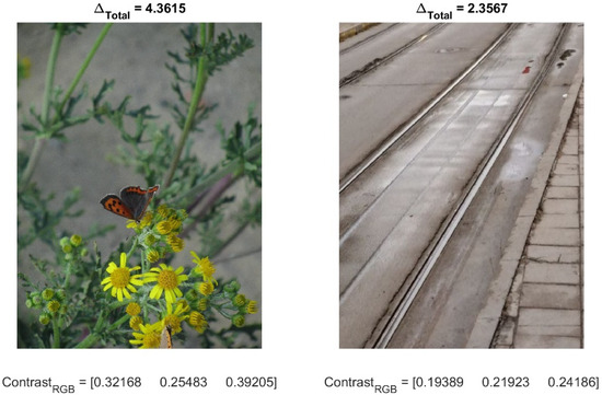
Figure 16.
Effect of contrast on method accuracy. The moving pattern is the same as in Figure 8, but the backgrounds differ. The figure presents two backgrounds, where the image on the right has a lower contrast for all three color channels than the one on the left. The contrast values are calculated for the whole scene. The value for as defined in Equation (9) is calculated for both cases of a different background, and is given in the title of the background pictures.
These results show we can expect less reliable behavior when the background scene’s contrast is more significant. The reason is that higher background contrast within the ROI may interfere with the changes caused by the moving object and obscure the tracking. Specific actions such as selecting a smaller initial region of interest can reduce the deviation caused by higher contrast values.
When analyzing the effect that the initial ROI size has on the performance of the tracking algorithm, we devised three different sets of tests. The first test involved varying the length and width of the rectangular region for a moving circular spot on a homogenous background. In the second test, various backgrounds were used, and the third analyzed real-world tracking scenarios. An example test for variation of initial ROI area for a moving object on a non-homogenous background is presented in Figure 17. We use the same moving pattern and object as presented in Figure 8—a Gaussian blob that changes positions in each frame. We vary the initial ROI size and record the tracking mismatch as defined in Equation (8), and the total mismatch as defined in Equation (9).
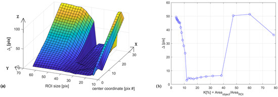
Figure 17.
(a) Region of interest size analysis. The graph has an x-axis which shows the coordinate of the center of the ROI in the current frame, a y-axis which shows the current ROI size, and a z-axis shows the tracking errors . The inverted plateau shows optimal ROI sizes for the present case. The moving pattern is again of a moving Gaussian “blob”, as is in Figure 8. (b) The graph shows the total mismatches for all frames along the y-axis, for different values of the ratio between object area and region of interest area—the value K along the x-axis.
An inverted plateau can be observed for certain initial ROI sizes (or ratios K between object area and ROI area). Outside of the inverted plateau, the mismatches are increased significantly, which shows that there is an upper and lower limit for useful ROI sizes. For the case of non-simulated videos, we examined whether or not the object of interest remained within the tracking area. For both simulated and real-world data tests combined, the mean lower boundary for the area ratio K defined in Equation (10) is 69%, while the mean upper boundary is 34%. This shows that there exists an optimal initial ROI size range for object tracking using this method. For the proposed tracking algorithm’s future development, additional analysis on the effect of background contrast and autonomous initial ROI selection is underway.
4. Summary and Discussion
We propose a novel method for object tracking. It addresses the challenge of real-time object-tracking optic flow techniques. The method successfully applies to numerous tests and real-world data, showing its effectiveness with various examples. An essential feature of our approach is the reconstruction of global transformation parameters, mitigating the computational complexity associated with most pixel-based optical flow algorithms. The method can be helpful for virtual tracking by dynamically adjusting a region of interest in a static wide-angle video stream and tracking with a mechanically steerable PTZ camera. Other methods [37,38] use video data to detect specific health conditions (such as epileptic seizures). In [37], a region of interest is drawn over a body part and the movements in that region are analyzed. This ROI is fixed, and if the patient’s body part leaves its boundaries, movement information will be lost. Our method can be used to update the ROI’s position and capture all the movements of the observed body part. In [38], the whole camera scene is used to acquire optic flow information and the recorded movements are used for seizure detection. This method could benefit from the tracking scheme presented in this work. Our algorithm can help by reducing computational requirements as a smaller part of the video data is used (due to the ROI). It provides additional benefits by isolating the object of interest (due to the ROI) and thus only relevant patient motion data are analyzed. In both cases, the methodology discussed here can provide substantial benefits.
Remote sensing and detecting adverse and potentially dangerous events is an ever-growing necessity. In certain situations, attached sensors are not the optimal solution, or may not even be a possible solution. Video observation provides remote sensing functionality, but in its commonly used operator-based form, it requires the constant alertness of trained personnel. For this reason, we have established a broad program dedicated to automated remote sensing algorithms. One of the currently operational systems is dedicated to real-time detection of convulsive epileptic seizures. The results presented in this work are intended for use in developing modules that deliver tracking capabilities and operate in conjunction with existing detection and alerting facilities.
One limitation of our approach is that we have used only group transformations that preserve the aspect ratio between the ROI axes, namely the translations and dilatations of the video image. As explained in the Methods section, one argument for this is the potential application of PTZ cameras. A second argument related to operator-controlled settings is that standard fixed aspect ratio monitors render the video images. We will explore an extended version of our ROI adaptive control paradigm in a forthcoming study.
The comparison between the performance of the proposed ROI tracking method and that of other existing techniques for only one available data set is for reference only. We note that our goal is to investigate the potential use of reconstructed optical flow group velocities for autonomous ROI tracking. To the best of our knowledge, no other published methodology provides such functionality. Even if other algorithms produce better tracking results in particular applications or according to some specific performance criteria, implementing them in our integrated system would require additional computational resources. In our modular approach, optical flow reconstruction is performed to detect epileptic motor fits, and applying it to other modules, such as ROI or PTZ tracking, involves minimal added complexity. This said, the illustrative comparison suggests that the proposed technique may be generally competitive with other tracking methods, especially if the required computational resources are considered.
Further limitations and restrictions of the method related to the velocity of the tracked object and the initial size of the region of interest are examined and listed earlier in this work. An open question that remains here is how to proceed if the algorithm “loses” the object of observation. One immediate solution is to detect the situation and alert an operator to intervene. Such an approach will, of course, undermine the autonomous operation of the system. Another possibility we are currently investigating is to introduce a dual-ROI concept where the algorithm keeps a broader observation margin that would allow for mitigating some of the limitations.
Our technique can also utilize adaptive features that provide performance reinforcement on the move while operating in real time. The adaptive extension is now considered on synthetic and real-life sequences and will be published elsewhere. Here, we note that it does not need large sets of pre-recorded training samples, as when using conventional learning techniques [14,20,21,39].
We would also point out that because the method proposed in our work is ROI-based, it allows parallel proliferation for simultaneous tracking of multiple separated objects if computational resources permit. A typical application of such a technique would be using a wide-angle high-resolution static camera for observation of multiple targets. If, however, the objects cross their positions in the camera’s field of view, rules of disambiguation should apply. This extension of the methodology goes beyond the scope of this report and is a subject of our further investigations.
As our approach uses global group transformation quantifiers, it is not critically sensitive to the image spatial resolution. Therefore, any noise removal by smoothening of the frames, for example with a Gaussian kernel, will not affect, or will even enhance, the reconstruction quality of the group parameters. In this context, our technique potentially allows for simple tackling of noisy inputs, for example (but restricted to) white additive noise.
Finally, we note that the method introduced in this work is intended to be incorporated together with patient monitoring systems (such as detecting epileptic seizures, apneas, or other adverse motor events/symptoms in patients). This will allow us to restrict the optical flow reconstruction task to those transformations relevant to the PTZ camera control. The technique is, however, applicable to a broader set of situations, including applications where the camera is moving, as for example considered in [40]. In the clinical practice of patient observation, cameras moving on rails and/or poles are available. It is, however, the added complexity of manual control that limits their use. To achieve automated control in real-time, a larger set of group transformations, including rotations and shear, may be used to track and control the camera position and orientation.
Author Contributions
Conceptualization: G.P. and S.K. (Stiliyan Kalitzin); Methodology: G.P., S.K. (Stiliyan Kalitzin) and S.I.; Software: S.K. (Simeon Karpuzov), G.P. and S.K. (Stiliyan Kalitzin); Validation: S.K. (Simeon Karpuzov) and Alexander Petkov.; Formal analysis: S.K. (Simeon Karpuzov) and Alexander Petkov.; Investigation: S.K. (Simeon Karpuzov); Resources: S.K. (Stiliyan Kalitzin); Data curation: S.K. (Stiliyan Kalitzin); Writing—original draft preparation: S.K. (Simeon Karpuzov); Writing—review and editing: G.P. and S.K. (Stiliyan Kalitzin); Visualization: S.K. (Simeon Karpuzov) and A.P.; Supervision: G.P. and S.K. (Stiliyan Kalitzin); Project administration: G.P. and S.K. (Stiliyan Kalitzin); Funding acquisition, S.I. and S.K. (Stiliyan Kalitzin). All authors have read and agreed to the published version of the manuscript.
Funding
The GATE project has received funding from the European Union’s Horizon 2020 WIDESPREAD-2018-2020 TEAMING Phase 2 Programme under Grant Agreement No. 857155 and the Operational Programme Science and Education for Smart Growth under Grant Agreement No. BG05M2OP001-1.003-0002-C01. Stiliyan Kalitzin is partially funded by “De Christelijke Vereniging voor de Verpleging van Lijders aan Epilepsie”, Program 35401, Remote Detection of Motor Paroxysms (REDEMP).
Institutional Review Board Statement
Not applicable.
Informed Consent Statement
Not applicable.
Data Availability Statement
The data presented in this study are available on request from the corresponding author.
Acknowledgments
The results presented in this paper are part of the GATE project.
Conflicts of Interest
The authors declare no conflicts of interest.
References
- Kalitzin, S.; Petkov, G.; Velis, D.; Vledder, B.; da Silva, F.L. Automatic segmentation of episodes containing epileptic clonic seizures in video sequences. IEEE Trans. Biomed. Eng. 2012, 59, 3379–3385. [Google Scholar] [CrossRef]
- Geertsema, E.E.; Visser, G.H.; Sander, J.W.; Kalitzin, S.N. Automated non-contact detection of central apneas using video. Biomed. Signal Process. Control 2020, 55, 101658. [Google Scholar] [CrossRef]
- Geertsema, E.E.; Visser, G.H.; Viergever, M.A.; Kalitzin, S.N. Automated remote fall detection using impact features from video and audio. J. Biomech. 2019, 88, 25–32. [Google Scholar] [CrossRef] [PubMed]
- Choi, H.; Kang, B.; Kim, D. Moving object tracking based on sparse optical flow with moving window and target estimator. Sensors 2022, 22, 2878. [Google Scholar] [CrossRef] [PubMed]
- Farag, W.; Saleh, Z. An advanced vehicle detection and tracking scheme for self-driving cars. In Proceedings of the 2nd Smart Cities Symposium (SCS 2019), Bahrain, 24–26 March 2019; IET: Stevenage, UK, 2019. [Google Scholar]
- Gupta, A.; Anpalagan, A.; Guan, L.; Khwaja, A.S. Deep learning for object detection and scene perception in self-driving cars: Survey, challenges, and open issues. Array 2021, 10, 100057. [Google Scholar] [CrossRef]
- Lipton, A.J.; Reartwell, C.; Haering, N.; Madden, D. Automated video protection, monitoring & detection. IEEE Aerosp. Electron. Syst. Mag. 2003, 18, 3–18. [Google Scholar]
- Wang, W.; Gee, T.; Price, J.; Qi, H. Real time multi-vehicle tracking and counting at intersections from a fisheye camera. In Proceedings of the 2015 IEEE Winter Conference on Applications of Computer Vision, Waikoloa, HI, USA, 5–9 January 2015; IEEE: Piscataway, NJ, USA, 2015. [Google Scholar]
- Kim, H. Multiple vehicle tracking and classification system with a convolutional neural network. J. Ambient Intell. Humaniz. Comput. 2022, 13, 1603–1614. [Google Scholar] [CrossRef]
- Yeo, H.-S.; Lee, B.-G.; Lim, H. Hand tracking and gesture recognition system for human-computer interaction using low-cost hardware. Multimed. Tools Appl. 2015, 74, 2687–2715. [Google Scholar] [CrossRef]
- Fagiani, C.; Betke, M.; Gips, J. Evaluation of Tracking Methods for Human-Computer Interaction. In Proceedings of the WACV, Orlando, FL, USA, 3–4 December 2002. [Google Scholar]
- Hunke, M.; Waibel, A. Face locating and tracking for human-computer interaction. In Proceedings of the 1994 28th Asilomar Conference on Signals, Systems and Computers, Pacific Grove, CA, USA, 31 October–2 November 1994; IEEE: Piscataway, NJ, USA, 1994. [Google Scholar]
- Salinsky, M. A practical analysis of computer based seizure detection during continuous video-EEG monitoring. Electroencephalogr. Clin. Neurophysiol. 1997, 103, 445–449. [Google Scholar] [CrossRef]
- Yilmaz, A.; Javed, O.; Shah, M. Object tracking: A survey. ACM Comput. Surv. 2006, 38, 13-es. [Google Scholar] [CrossRef]
- Deori, B.; Thounaojam, D.M. A survey on moving object tracking in video. Int. J. Inf. Theory 2014, 3, 31–46. [Google Scholar] [CrossRef]
- Mangawati, A.; Leesan, M.; Aradhya, H.R. Object Tracking Algorithms for video surveillance applications. In Proceedings of the 2018 International Conference on Communication and Signal Processing (ICCSP), Melmaruvathur, India, 3–5 April 2018; IEEE: Piscataway, NJ, USA, 2018. [Google Scholar]
- Li, X.; Hu, W.; Shen, C.; Zhang, Z.; Dick, A.; Hengel, A.V.D. A survey of appearance models in visual object tracking. ACM Trans. Intell. Syst. Technol. 2013, 4, 1–48. [Google Scholar] [CrossRef]
- Piccardi, M. Background subtraction techniques: A review. In Proceedings of the 2004 IEEE International Conference on Systems, Man and Cybernetics (IEEE Cat. No. 04CH37583), The Hague, The Netherlands, 10–13 October 2004; IEEE: Piscataway, NJ, USA, 2004. [Google Scholar]
- Benezeth, Y.; Jodoin, P.-M.; Emile, B.; Laurent, H.; Rosenberger, C. Comparative study of background subtraction algorithms. J. Electron. Imaging 2010, 19, 033003. [Google Scholar]
- Chen, F.; Wang, X.; Zhao, Y.; Lv, S.; Niu, X. Visual object tracking: A survey. Comput. Vis. Image Underst. 2022, 222, 103508. [Google Scholar] [CrossRef]
- Ondrašovič, M.; Tarábek, P. Siamese visual object tracking: A survey. IEEE Access 2021, 9, 110149–110172. [Google Scholar] [CrossRef]
- Doyle, D.D.; Jennings, A.L.; Black, J.T. Optical flow background estimation for real-time pan/tilt camera object tracking. Measurement 2014, 48, 195–207. [Google Scholar] [CrossRef]
- Husseini, S. A Survey of Optical Flow Techniques for Object Tracking. Bachelor’s Thesis, Tampere University, Tampere, Finland, 2017. [Google Scholar]
- Kalitzin, S.; Geertsema, E.E.; Petkov, G. Optical Flow Group-Parameter Reconstruction from Multi-Channel Image Sequences. In Proceedings of the APPIS, Las Palmas de Gran Canaria, Spain, 8–12 January 2018. [Google Scholar]
- Horn, B.K.; Schunck, B.G. Determining optical flow. Artif. Intell. 1981, 17, 185–203. [Google Scholar] [CrossRef]
- Lucas, B.D.; Kanade, T. An iterative image registration technique with an application to stereo vision. In Proceedings of the IJCAI’81: 7th International Joint Conference on Artificial Intelligence, Vancouver, BC, Canada, 24–28 August 1981. [Google Scholar]
- Koenderink, J.J. Optic flow. Vis. Res. 1986, 26, 161–179. [Google Scholar] [CrossRef]
- Beauchemin, S.S.; Barron, J.L. The computation of optical flow. ACM Comput. Surv. 1995, 27, 433–466. [Google Scholar] [CrossRef]
- Florack, L.; Niessen, W.; Nielsen, M. The intrinsic structure of optic flow incorporating measurement duality. Int. J. Comput. Vis. 1998, 27, 263–286. [Google Scholar] [CrossRef]
- Niessen, W.; Maas, R. Multiscale optic flow and stereo. In Gaussian Scale-Space Theory, Computational Imaging and Vision; Kluwer Academic Publishers: Dordrecht, The Netherlands, 1996. [Google Scholar]
- Maas, R.; ter Haar Romeny, B.M.; Viergever, M.A. A Multiscale Taylor Series Approaches to Optic Flow and Stereo: A Generalization of Optic Flow under the Aperture. In Proceedings of the Scale-Space Theories in Computer Vision: Second International Conference, Scale-Space’99 Proceedings 2, Corfu, Greece, 26–27 September 1999; Springer: Berlin/Heidelberg, Germany, 1999. [Google Scholar]
- Aires, K.R.; Santana, A.M.; Medeiros, A.A. Optical flow using color information: Preliminary results. In Proceedings of the 2008 ACM Symposium on Applied Computing, Fortaleza, Brazi, 16–20 March 2008. [Google Scholar]
- Niessen, W.; Duncan, J.; Florack, L.; Viergever, M. Spatiotemporal operators and optic flow. In Proceedings of the Workshop on Physics-Based Modeling in Computer Vision, Cambridge, MA, USA, 18–19 June 1995; IEEE Computer Society: Piscataway, NJ, USA, 1995. [Google Scholar]
- Pavel, M.; Sperling, G.; Riedl, T.; Vanderbeek, A. Limits of visual communication: The effect of signal-to-noise ratio on the intelligibility of American Sign Language. J. Opt. Soc. Am. A 1987, 4, 2355–2365. [Google Scholar] [CrossRef] [PubMed]
- Kalitzin, S.N.; Parra, J.; Velis, D.N.; Da Silva, F.L. Quantification of unidirectional nonlinear associations between multidimensional signals. IEEE Trans. Biomed. Eng. 2007, 54, 454–461. [Google Scholar] [CrossRef] [PubMed]
- Fan, H.; Bai, H.; Lin, L.; Yang, F.; Chu, P.; Deng, G.; Yu, S.; Harshit; Huang, M.; Liu, J. Lasot: A high-quality large-scale single object tracking benchmark. Int. J. Comput. Vis. 2021, 129, 439–461. [Google Scholar] [CrossRef]
- Pediaditis, M.; Tsiknakis, M.; Leitgeb, N. Vision-based motion detection, analysis and recognition of epileptic seizures—A systematic review. Comput. Methods Programs Biomed. 2012, 108, 1133–1148. [Google Scholar] [CrossRef]
- Cuppens, K.; Vanrumste, B.; Ceulemans, B.; Lagae, L.; Van Huffel, S. Detection of epileptic seizures using video data. In Proceedings of the 2010 Sixth International Conference on Intelligent Environments, Kuala Lumpur, Malaysia, 19–21 July 2010; IEEE: Piscataway, NJ, USA, 2010. [Google Scholar]
- Yang, F.; Zhang, X.; Liu, B. Video object tracking based on YOLOv7 and DeepSORT. arXiv 2022, arXiv:2207.12202. [Google Scholar]
- Jana, D.; Nagarajaiah, S. Computer vision-based real-time cable tension estimation in Dubrovnik cable-stayed bridge using moving handheld video camera. Struct. Control Health Monit. 2021, 28, e2713. [Google Scholar] [CrossRef]


Disclaimer/Publisher’s Note: The statements, opinions and data contained in all publications are solely those of the individual author(s) and contributor(s) and not of MDPI and/or the editor(s). MDPI and/or the editor(s) disclaim responsibility for any injury to people or property resulting from any ideas, methods, instructions or products referred to in the content. |
© 2024 by the authors. Licensee MDPI, Basel, Switzerland. This article is an open access article distributed under the terms and conditions of the Creative Commons Attribution (CC BY) license (https://creativecommons.org/licenses/by/4.0/).