Abstract
The progress in machine learning during the last decade has had a considerable impact on many areas of science and technology, including quantum technology. This work explores the application of reinforcement learning (RL) methods to the quantum control problem of state transfer in a single qubit. The goal is to create an RL agent that learns an optimal policy and thus discovers optimal pulses to control the qubit. The most crucial step is to mathematically formulate the problem of interest as a Markov decision process (MDP). This enables the use of RL algorithms to solve the quantum control problem. Deep learning and the use of deep neural networks provide the freedom to employ continuous action and state spaces, offering the expressivity and generalization of the process. This flexibility helps to formulate the quantum state transfer problem as an MDP in several different ways. All the developed methodologies are applied to the fundamental problem of population inversion in a qubit. In most cases, the derived optimal pulses achieve fidelity equal to or higher than 0.9999, as required by quantum computing applications. The present methods can be easily extended to quantum systems with more energy levels and may be used for the efficient control of collections of qubits and to counteract the effect of noise, which are important topics for quantum sensing applications.
1. Introduction
The recent developments in quantum technologies, like quantum computing, quantum metrology, and quantum sensing, have advanced at a rapid pace. In this quantum race, the precise control of the fundamental quantum systems that are the building blocks for these important quantum technology applications is quite crucial. There are already a multitude of methods used in quantum control problems: resonant methods [1], adiabatic methods like rapid adiabatic passage [1,2] and stimulated Raman adiabatic passage [3], variances in adiabatic techniques termed shortcuts to adiabaticity [4], and optimal control methods [5,6] have been applied with great success for several years now.
Artificial intelligence (AI) is also a rapidly growing area, especially in the last decade with the advances in deep learning combined with the increase in the computational power of modern computer systems [7,8]. Reinforcement learning (RL) is the area of machine learning (ML) that is trying to develop algorithms and agents that learn to solve problems and make decisions based on training and interaction with the environment. This technique has been applied in many areas from games like chess and GO [9] to robotic systems for real-time decision processes and even to physics systems [10,11]. The present article is aligned with the ongoing efforts to apply RL in controlling quantum systems. More specifically, the goal of an RL agent is to drive a quantum system from some initial state to another target state by optimally shaping the applied electromagnetic field. The metric that is usually used for measuring the success of a state transition is the fidelity () of the final state with respect to the target state. There are also other types of machine learning, such as supervised learning, which have been used to solve quantum control problems, like qubit characterization [12] and qubit manipulation and readout [13]. This article only deals with RL methods.
Reinforcement learning solves problems that are in the mathematical form of a Markov decision process (MDP) [14]. For this reason, one should formulate the problem of quantum state transfer as an MDP, which governs the agent-environment interplay of the problem. In this context, the quantum mechanical system is actively involved in the defined environment. This work presents different formulations of the MDP in an attempt to explore many possible ways to formalize the state transfer problem, building on previous works [15,16,17,18,19,20,21,22,23,24].
The fundamental building block of quantum systems and the smallest chunk of quantum information is the two-level system or qubit [2]. For this reason, the proposed methodology is used to control the dynamics of a single qubit, emphasizing the state transfer problem of population inversion from one qubit state to the other. The environment (MDP) and the agent are formulated in many different settings and combinations, and the results are presented from the application of several RL algorithms. In most cases, the agents are stressed to achieve fidelities higher than 0.9999, which is a rough estimate of the accuracy threshold needed for fault-tolerant quantum computation. The current work may serve as a stepping stone to apply the proposed methodology in more complex quantum control problems, for example, the simultaneous control of a collection of qubits with different frequencies and efficient qubit control in the presence of noise, which are essential in quantum sensing. We plan to address these problems in future work.
The structure of this article is as follows: In Section 2, we present the theoretical aspects of the qubit system and the mathematical aspects of the MDP and RL, as well as the different formulations and settings of the MDP process and how they are related to the two-level system. Section 3 provides an overview of the RL methods that are used in this paper, while Section 4 describes the trigonometric series optimization algorithm that uses RL methods to produce smooth control. Section 5 presents the results of the various algorithms for qubit population inversion; finally, Section 6 provides some insights and conclusions.
2. Two-Level System and Markov Decision Process (MDP)
2.1. Two-Level System
A two-level system or qubit is a quantum system that has two energy levels, as shown in Figure 1. The lower-energy state |1⟩ is called the ground state, and the higher-energy state |2⟩ is called the excited state. An arbitrary state of the qubit can be represented by a 2 × 2 density matrix
where the diagonal element is the population of state |i⟩, , and the off-diagonal elements express the coherence between the ground and excited states. Note that for a closed system (without losses), as the one considered here, it is ; thus, its general state can be represented by the triplet of real parameters .
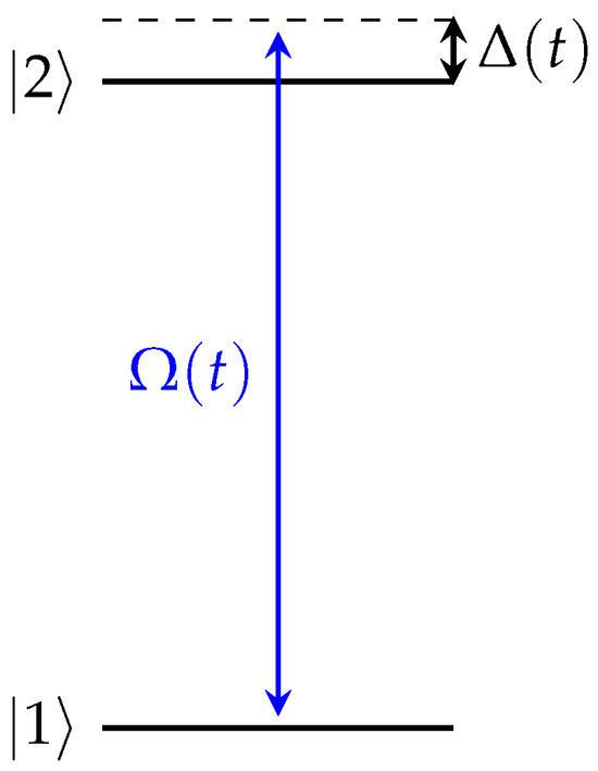
Figure 1.
Two-level system. is the Rabi frequency, proportional to the envelope of the applied electromagnetic field, and is the detuning between the qubit frequency and the frequency of the applied field.
The control of a qubit is usually achieved through the application of an external electromagnetic field. The Hamiltonian expressing the interaction of a two-level system with a chirped field of the form , where is the envelope, the angular frequency and the time-dependent phase of the field, under the electric dipole and rotating wave approximations, can be written as [2]
Here, ℏ is the Planck’s constant, the control function is called the Rabi frequency, with being the electric dipole matrix element between the energy levels, and is the detuning from the qubit frequency . In the presence of chirp (), the detuning is also time-dependent and serves as an extra control function in addition to the Rabi frequency. This Hamiltonian is expressed in compact form using Pauli matrices .
The qubit dynamics under Hamiltonian (2) is governed by the density matrix equation
where is a bilinear map , called a Lie bracket or the commutator. It maps two operators () in the Hilbert space that governs the quantum system to another one in the same Hilbert space. The qubit is initially () in its ground state |1⟩; thus, and . A well-known solution to the problem of population inversion, i.e., the transfer of a population to the excited state |2⟩, is the resonant pulse. This is a pulse without chirp applied on resonance with the qubit frequency, with constant amplitude and duration units of time. Here, RL methods are used to reproduce this optimal solution and retrieve other solutions considering time-dependent detuning.
2.2. Markov Decision Process (MDP)
The MDP is a framework for the problem of learning from interaction with the environment to achieve a goal. The entity that is learning from this interplay and makes the decisions is called an agent. The entity that the agent interacts with is called the environment. MDP is a tuple , where
- is the state space;
- is the action space;
- is a map that gives the probability that a state , and a reward happens based on previous state and the action ;
- is the discount factor.
The agent interacts at discrete time steps . At each step, the agent receives a representation of the environment, which is called the state, denoted by . Based on the state, the agent selects an action . In the next step, the response of the environment to the agent’s action is a numerical reward, . In the new step, the environment is in a new state . The whole process is illustrated in Figure 2. Following this procedure, a sequence of states, actions, and rewards are generated, forming a trajectory:
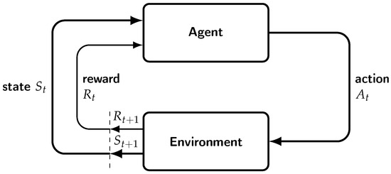
Figure 2.
MDP and agent–environment interplay.
The probability function p determines the dynamics of the MDP. Since p defines a probability distribution for each choice of s and a, it is
This probability distribution completely characterizes the dynamics of the environment. The probability of each state and reward depends only on the immediately preceding state and action . This is a restriction on the state of the environment. The state must have information about the past agent–environment interaction. If this is true, then the state has the Markov property.
2.3. Qubit System and State Transfer as an MDP
The state and action spaces of the qubit system have to be defined in the context of an MDP. The environment does not always coincide with the quantum system. It depends on the formulation of the MDP. In general, the environment and the quantum system are two different entities. State and action spaces can both be defined as discrete or continuous.
2.3.1. Finite State Space
Following Ref. [15], a discrete state space can be defined as the tuple , where is the set of the time steps in an episode or trajectory, and is the discrete space of the available Rabi frequencies. Only step size pulses are allowed, with taking values in the interval . Obviously, the considered pulses are resonant and without chirp. The MDP state at time step t is given by the tuple:
where and .
2.3.2. Continuous State Space
A more intuitive choice would be to use the state of the quantum system to construct the state of the MDP. The quantum state also has the Markov property, since the current state and the next actions do not depend on the history of the process. The quantum state space is an infinite dimensional space, thus continuous MDP state space is more relevant in this case. This formulation offers more freedom in the choice of actions, which may potentially lead to new insights about the dynamics and control of the system. By incorporating the qubit state, the MDP state space can be defined as a subset of or , with the corresponding MDP state represented by a 4-tuple or a 5-tuple, depending on whether system is resonant or time-dependent ,
or
respectively. Note that for a certain case below, a hybrid MDP state space of the form (6) is used, with discrete Rabi frequency and continuous density matrix elements.
2.3.3. Action Space
The action space can be discrete or continuous. In the resonant setup where the only control is the Rabi frequency, each action corresponds to the correction of the value of the Rabi frequency from the previous time step. If is the Rabi frequency at time t, and the action taken at next time step is , then, at time :
In the setup where detuning is used as an additional control, the action is defined as a tuple of two corrections . In this case, the action corrects both the Rabi frequency and the detuning; thus, aside from the change described in Equation (8), there is a corresponding one for the detuning:
2.3.4. Reward Function
The metric that shows the success of a quantum state transfer process is the fidelity of the evolved density matrix with respect to the target density matrix , which is defined as the trace of the matrix product
Note that is obtained from the evolution of Equation (3), when starting from the initial condition . For the population inversion problem the fidelity is simply the population of the excited state,
The MDP reward function, which is responsible for the way the RL agent assimilates the quantum dynamics, depends on the quantum state fidelity. The goal is to derive an optimal policy that exceeds a prescribed threshold fidelity within the least possible time. For this reason, each time step is additionally penalized by giving a negative reward set to , but, when the desired fidelity threshold is surpassed, the agent receives a constant big positive reward. The MDP is defined as an episodic process, and each episode corresponds to a pulse sequence that drives the system from the initial state to another, very close to the desired one in the best-case scenario. An episode ends when the maximum allowed time has passed or the desired fidelity has been achieved. Combining all the above, the reward function is defined as follows:
where is a constant reward given to the agent if the threshold fidelity is exceeded during the episode, and u is the unit step function defined as
Note that in the reward function , instead of , is used, because it gives higher rewards since , leading to faster convergence to the optimal policies during training. Note that in Equation (13), the actual fidelity is used for comparison with the target threshold.
3. Reinforcement Learning (RL) Methods
3.1. Temporal Difference (TD) Methods
Temporal difference learning [14] is a set of algorithms from reinforcement learning that combine ideas from Monte Carlo learning and dynamic programming. TD methods learn directly from experience without any model of the environment. They also update estimates based on other learned estimates but without waiting for the final outcome (bootstrapping). TD methods do not need to wait until the end of the episode to determine the change in the value function V(), such as in Monte Carlo (MC) methods. At the next time step , TD makes the update using the observed reward of new step and the estimate for the next time step value state . A simple update that can be used is the following rule:
where is the learning rate, is the discount in the next state value, and the actual return following time t. Most TD algorithms employ similar update rules but, in most cases, use the action-value function instead of the state-value function.
3.1.1. Q-Learning
Q-learning [25] is one of the most applicable algorithms from the TD family. The basic concept is that after the agent tries an action in a state, it receives the immediate reward and moves to a new state. It evaluates and compares the immediate result with the estimate of the value of the previous state. Exploring all actions in all possible states repeatedly, it finally learns the optimal policy based on the long-term discounted return. The main steps of Q-learning are summarized in Algorithm 1. It is considered an off-policy method since it tries to improve a policy that is different from the one that was used to generate the data. It is important to note that an exploration of action selection is required to examine all state–action pairs and determine the optimal ones. This is achieved by introducing an -greedy policy during the sampling during the algorithm training, where is a real number between 0 and 1, usually close to 0. The value means that the policy is random and always chooses actions randomly, no matter in what MDP state it is, while . This means that the policy chooses the most valued action most of the time (with probability ), but, in some cases, it chooses a random action (with probability ) in an attempt to explore all the state–action pairs sufficiently.
| Algorithm 1 Q-learning |
| Parameters: learning rate and |
| Initialize arbitrarily state-action value function |
| For each episode: |
| Initialize state s in |
| For each time step of episode: |
| Choose action with policy using Q-value function (i.e., -greedy) |
| Take action A, observe R, |
| until S terminal |
3.1.2. Expected State–Action–Reward–State–Action (SARSA)
Another algorithm that can be considered as a variation of Q-learning is the expected SARSA algorithm [14]. In this case, instead of the maximum over the next state-action value, the update rule uses the expected value of the next state-action pair, taking into account how likely each action is to be selected under the current policy:
Expected SARSA appears to eliminate the variance in the SARSA algorithm due to the random selection of action . It is expected to perform better than the latter given the same amount of learning experience.
3.1.3. Deep Q-Network
The Deep Q-Network [26] is one of the first deep reinforcement learning algorithms. It combines reinforcement learning with deep neural networks by using a complete fully connected artificial neural network (ANN) to approximate the action-value function Q. Nonlinear approximators such as neural networks with non-inear activation functions experience instabilities in the model. DQN algorithm addresses this problem with two key ideas:
- Experience replay: randomizes the data and removes correlations between sequential states;
- Periodically Q action-value function update: reduces the correlations with the target.
The experience replay mechanism stores agent experiences in a dataset where is the experience tuple at time step t. The Q-learning updates are done on random samples from these experiences. The loss function for the Q-learning update is defined by:
where is the discount factor, are the parameters of the Q-network that are used to get the target at iteration i, and are the parameters of the Q-network at iteration i. Parameters are updated periodically with the values of parameters and are fixed in between. This practically means that the parameters are updated at each step of the training, but they are not directly used in the estimated value inside the max operation. Only after some iterations, these parameters are used to update the periodically steady parameters of the target network. This process is achieved by preserving two instances of the same neural network: one with parameters and another one with parameters . The first network is constantly updated, and the second one is updated periodically using the parameter values of the first. In this way, the correlations between subsequent experiences are reduced. More details on this procedure are given in Algorithm 2. Concerning the architecture of the network, the input neuron layer incorporates the state and the action of the current time step, while the output neuron values correspond to the action values of each possible next action. It is trivial to think that this algorithm works without any further modification with discrete state and action spaces. In Figure 3a, the DQN architecture for the discrete MDP state space is presented, defined in Equation (5); in Figure 3b, the DQN architecture for a hybrid MDP state space of the form (6) is presented, with discrete Rabi frequency and continuous density matrix elements. These figures make obvious the advantage of the DQN architecture; that is, for each state–action pair, the action value of every possible next action is estimated at once.
| Algorithm 2 Deep Q-Network with experience replay |
| Initialize replay buffer/memory D |
| Initialize ANN with random weights |
| Initialize target ANN with random weights and update rate C |
| for each episode: do |
| Initialize state s in |
| for each time step of episode: do |
| Choose action based on the -greedy policy in the parametrized action value |
| Take action a, observe r, |
| Store experience in memory D |
| Select a random mini-batch experience from memory D |
| Obtain the return based on next maximum valued action: |
|
|
| Perform gradient descent on the loss function (16) |
| Update parameters so that every C steps |
| end for |
| end for |
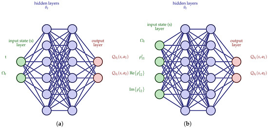
Figure 3.
DQN architectures of neural networks. (a) DQN architecture 1. (b) DQN architecture 2. The first architecture has a discrete state space with , and the second has a hybrid state space of the form , with discrete Rabi frequency and continuous density matrix elements. In both architectures, the output layer produces the values of all available actions that correspond to the input state. The greedy policy should select the action with the higher value, breaking ties randomly.
3.2. Policy Gradient Methods
The previously explored methods are called value-based methods since they learn the value functions and extract the policy from them. There is another kind of method, the policy gradient methods, which do not depend on the action values at all, but they use a an improved parameterized policy to select the best actions [14].
3.2.1. Policy Approximation
Policy is parameterized by a set of parameters and should be differentiable with respect to them. It represents the probability of selecting action when being in state ,
The methods learn the optimal policy parameters by using approximate gradient ascent in a performance measure
where is the learning rate, are the previous step parameters, and are the current time step parameters. There is a challenge in calculating the gradient of the objective function since it depends not only on the action selection but also on the distribution of states. There is a theoretical result that overcomes this challenge, called the policy gradient theorem, which states that the gradient of the objective function does not depend on the distribution of states [14]:
where are the policy parameters, the policy, and the distribution of the importance of states under policy (, ).
3.2.2. Discrete Action Space Parameterization
If the state space is not too large, the policy is commonly parameterized according to an exponential softmax distribution
where is the parameterized numerical preferences for each action–state pair, and b represents an action index. Policy is in fact a probability distribution, since the sum of the action probabilities on each state sum up to one. This parameterization is called softmax in action preferences. The action preferences can be parameterized arbitrarily. They can be computed by an artificial neural network, where is the weight of the ANN. One advantage of this parameterization is that the approximate policy can potentially approach a deterministic policy, in contrast to -greedy action selection, where there is always a possibility of selecting a random action.
3.2.3. Continuous Action Space Parameterization
Policy gradient methods are applicable not only on discrete action spaces: with the appropriate parameterization, they can also handle very large or even continuous action spaces [14]. In this case, models learn the statistics of the probability distribution, and actions are sampled from this distribution. One common choice is sampling actions from a normal Gaussian distribution. The probability density function is given by
where is the mean, and is the standard deviation of the normal distribution. The probability of selecting an action from a subset of the complete action space is given by the following integral:
where is the action subset, and is the probability measure in the action distribution space. The integral can be thought of as the more general Lebesgue integral since a can be arbitrary and not only on . Using this probability distribution, a policy can be thought of as a probability density function where the mean and the standard deviation can be approximated by state-dependent parameterized functions and that can be represented by artificial neural networks
3.2.4. REINFORCE Algorithm
REINFORCE [27] is a policy gradient algorithm based on the policy gradient theorem, which uses the total return of an episode to proceed to the parameter updates; thus, it can be regarded as a Monte Carlo method. This is why it is also called the Monte Carlo policy gradient algorithm. The following pseudocode (Algorithm 3) describes the process of the algorithm. Figure 4a displays the REINFORCE neural network architecture for the discrete MDP state space defined in Equation (5), while Figure 4b depicts the corresponding architecture for the continuous MDP state space defined in Equation (6). Observe that in the first case, the output is the discrete probability distribution of the action selection, while the second is the parameters defining a continuous probability distribution, for example, the mean and standard deviation for a parameterized normal probability distribution, as in Equation (23).
| Algorithm 3 REINFORCE algorithm |
| Initialize parameters of the policy and learning parameter |
| for each episode: do |
| Generate a full episode |
| for each time step of episode do |
|
|
| end for |
| end for |
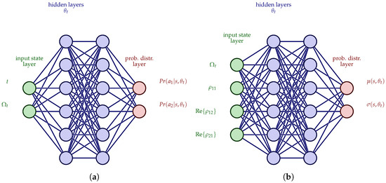
Figure 4.
REINFORCE architecture of neural networks. (a) REINFORCE—Policy NN architecture 1. (b) REINFORCE—Policy NN architecture 2. The first architecture has a discrete state space with , and the second has a continuous state space with , where, here, the Rabi frequency is also continuous. In the first case, the output is the discrete probability distribution of the actions selection, while in the second, the output is the parameters of a continuous probability distribution, for example, the mean and standard deviation of a parameterized normal probability distribution as in Equation (23).
There is an intuition behind the update rule of the algorithm. Each increment is proportional to the product of the return and a vector, the gradient of the probability of taking the action divided by the probability of taking that action. The vector shows the direction in the parameter space that increases the probability of repeating the action at state . The update term increases proportionally to the actual return and inversely proportionally to the action probability. This is the intuitive approach since the parameters move in the direction in which actions give higher returns, and it does not give an advantage to actions that are frequently selected.
3.3. Actor-Critic Methods
The reinforcement learning methods analyzed so far fall into two main categories [28,29]: the value-based (critic-only) methods, which approximate value functions and derive policies from them; and the policy-based (actor-only) methods, which use parameterized policies and try to learn optimal policies. There is also a third class of methods, which are called actor-critic methods. They try to combine the strengths of both previous approaches. The critic approximates the value function, which is used by the actor to update the parameters of the parameterized policy. Actor-critic methods are based on the important observation that since the number of actor parameters is less than the number of states, the critic does not need to approximate the exact value function. A parameterized actor computes continuous actions without the need for the optimization of a value function, while a critic offers to the actor knowledge about the performance with low variance, a combination that speeds up learning. Both actor and critic have access to the state of the system. This process is illustrated in Figure 5.
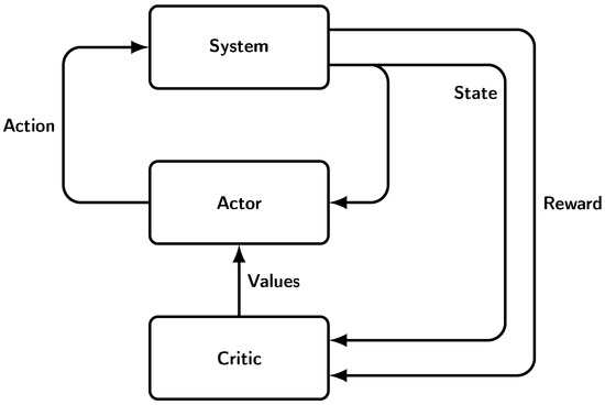
Figure 5.
Actor-critic architecture.
Proximal policy optimization (PPO) algorithms [30] are a family of policy gradient methods that optimize a surrogate objective function by stochastic gradient ascent. PPO updates multiple epochs of mini-batch updates, optimizing a surrogate objective function by stochastic gradient ascent. This algorithm is inspired by the trust region policy optimization (TRPO) algorithm [31]. TRPO maximizes a surrogate loss given by
where
is the probability ratio, the state, and the action at time step t. CPI stands for conservative policy iteration. Without any constraint, the loss function leads to large policy updates, so the idea here is to modify the loss function so that the policy updates do not move away from 1 ().
The PPO algorithm has the same benefits as TRPO, but it is simpler to implement and has better sample complexity. Some of the surrogate losses considered for the PPO algorithms are the CLIP loss and the KLPEN loss. CLIP loss includes a penalty term in the parameter updates that clips the loss as follows:
where is called the advantage function . KLPEN loss is defined by adding a penalty on KL divergence
KL divergence is a type of statistical distance, a measure of how one probability distribution is different from a second reference probability distribution. These losses can be computed and differentiated. Practical implementations utilize multiple steps of gradient ascent to optimize the parameters based on the loss function. There is also an option to share parameters across the two used neural networks, one for the critic and the other for the value function. In this case, the loss function should combine the policy surrogate loss and the value function error loss or even add an additional entropy term that ensures sufficient exploration
where are some coefficients, S is the entropy term and is the squared error loss .
4. Trigonometric Series Optimization Algorithm (TSOA)
The control functions, which always include the Rabi frequency and additionally the time-dependent detuning in the case of chirped pulses, can be represented by finite trigonometric series. The idea for this representation was already used in Ref. [32] to solve quantum control problems with optimal control and in Ref. [33] to implement fast adiabatic qubit gates. This formulation produces smooth controls for and , which are easier to be implemented experimentally. We thus consider the truncated series
where p is the number of harmonics used in the truncated expansions. The parameter vector to be determined is normalized to unity,
The continuity of the action space in this formulation requires a policy gradient or an actor-critic method so that the MDP can be solved. The actor neural network architecture is displayed in Figure 6. Observe here that the input is the quantum state, expressed by the real numbers , while the output is the optimal values of the parameter vector components. The MDP in this situation is defined by only one time step; the model maps the MDP state that coincides with the quantum state to the action that is the set of the parameters of the trigonometric series. This is a completely different formulation of the problem as an MDP. This model approximates the optimization process to find the optimal parameters to represent the optimal controls via the trigonometric series. The time in which the quantum system evolves is fixed, so this is a fixed time optimization process.
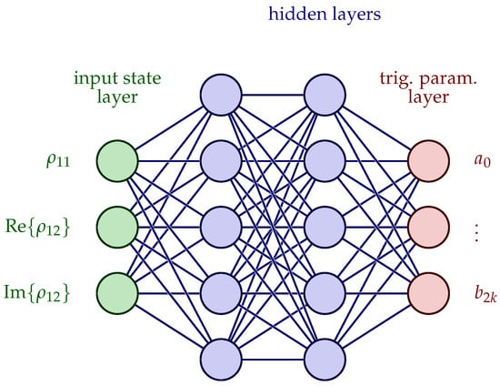
Figure 6.
Parameterized policy actor NN. Input layer consists of the state of the quantum system (the necessary density matrix components), and output layer consists of the parameters of the truncated trigonometric series for the controls and .
5. Results and Discussion
In the following sections, the results obtained from the trained RL agents are presented, along with the parameters used for each model. At first, tabular methods using discrete action and state space MDP setup were used. Then, the same setup was used in deep RL methods, such as DQN. In the DQN algorithm, which is a value-based method, the actions should remain discrete, but the state space can be extended to be continuous, utilizing the formulation with density matrix elements. Next, policy gradient methods were employed initially using the same MDP setups, but MDP setups where both the action and state spaces are continuous were considered too. Actor-critic methods were only tested with the continuous MDP formulation since this is the area where they really excel.
In all simulations of quantum system evolution, . The Rabi frequency and the detuning were normalized with respect to parameter , so the time unit was . This unit convention is used in all figures throughout this paper.
All the algorithms were developed using the open-source machine learning platform TensorFlow [34]. This also includes a specific library for reinforcement learning, named TF-Agents, which accelerates the algorithm implementation and execution. The quantum system evolution was simulated by QuTiP [35], which is open-source software for simulating the dynamics of quantum systems. The versions of the software are shown in Table 1. The simulations were performed with a computer utilizing the CPU, with specifications shown in Table 2.

Table 1.
Software versions.

Table 2.
Computer hardware specifications.
5.1. Temporal Difference Methods
5.1.1. Tabular Methods (Q-Learning and Expected SARSA)
The Q-learning algorithm with the discrete action and state space MDP setup (5) was used first. The threshold fidelity was set at , and a discrete action space with seven actions was used. The parameters of the algorithm are shown in the Table 3, while the results are displayed in Figure 7 and Figure 8, at an early training stage of 2000 episodes and the final training stage of 20,000 episodes, respectively. Observe that in the early stage, the algorithm did not succeed in obtaining an optimal policy yet, since the fidelity failed to attain the 0.99 threshold, as shown in Figure 7b, and substantially deviates from the optimal -pulse, as shown in Figure 7a. On the other hand, at the later stage of 20,000 episodes of training, the agent produced an optimal policy that achieved the threshold fidelity, Figure 8b, while attained the shape of the optimal -pulse, Figure 8a. Note that since the threshold fidelity was only 0.99, it was obtained earlier than units of time. Also, observe that the expected return (cumulative rewards) from the training episodes improved with the number of episodes by comparing Figure 7c and Figure 8c. These figures contain all cumulative returns for all training episodes and show how the episode rewards change as training accumulates.

Table 3.
Tabular methods parameters—7 actions.
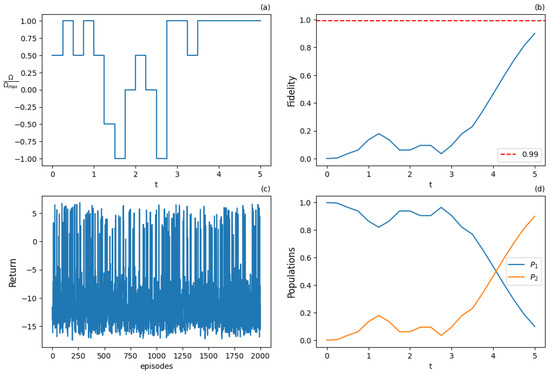
Figure 7.
Results for Q-learning with 7 actions at the early training stage after 2000 training episodes: (a) optimal normalized Rabi frequency as the external control of the system, (b) fidelity (population of excited state |2⟩) as a metric the performance of the population transfer, (c) expected return (cumulative rewards) results during the training episodes, (d) populations of states |1⟩ and |2⟩. Pulse shape does not succeed in transferring the state due to lack of sufficient learning.
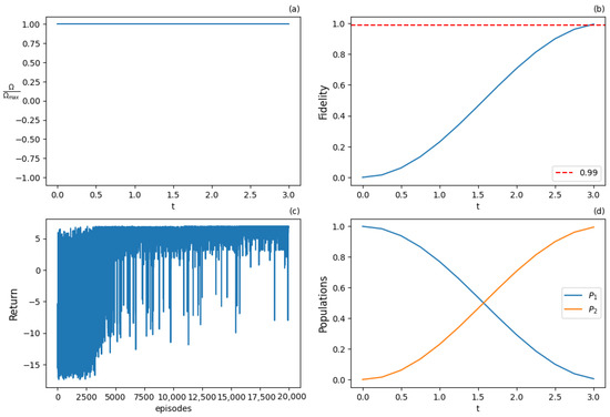
Figure 8.
Results for Q-learning with 7 actions at the final training stage after 20,000 training episodes: (a) optimal normalized Rabi frequency as the external control of the system, (b) fidelity (population of excited state |2⟩) as a metric the performance of the population transfer, (c) expected return (cumulative rewards) from the training episodes, (d) populations of states |1⟩ and |2⟩. Solution successfully inverts the population between the two states.
The expected SARSA algorithm outperforms the Q-learning algorithm for the early stage of training, since now the agent is able to attain the target fidelity, as shown in Figure 9. The parameters of the algorithm are the same as those of the Q-learning algorithm. Note that for the early-stage training, the threshold fidelity is obtained for a longer duration than units of time, as shown in Figure 9b, while deviates from the constant -pulse, see Figure 9a. For the later stage of training the results of expected SARSA, displayed in Figure 10, are similar to those obtained with Q-learning and shown in Figure 8.
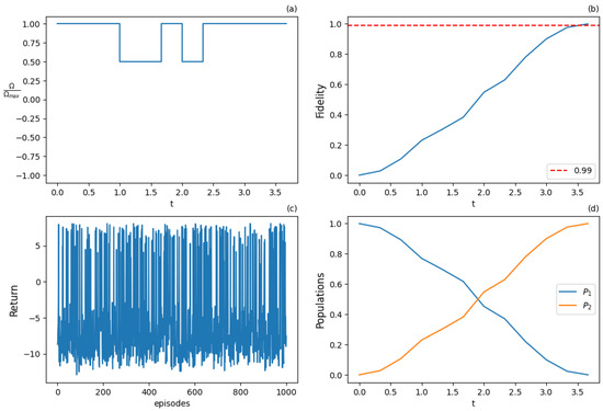
Figure 9.
Results for expected SARSA with 7 actions at the early training stage after 1000 training episodes: (a) optimal normalized Rabi frequency as control of the system, (b) fidelity (population of excited state |2⟩) as a metric the performance of the population transfer, (c) expected return (cumulative rewards) from the training episodes averaged from 10 episode samples, (d) populations of states |1⟩ and |2⟩. Suboptimal solution even at the early stage of training process.
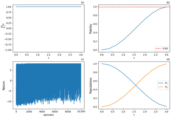
Figure 10.
Results for expected SARSA with 7 actions at the final training stage after 10,000 training episodes: (a) optimal normalized Rabi frequency , (b) fidelity (population of excited state |2⟩) as a metric the performance of the population transfer, (c) expected return (cumulative rewards) from the training episodes averaged from 10 episode samples, (d) populations of states |1⟩ and |2⟩. Agent can provide the optimal solution (-pulse).
5.1.2. DQN Algorithm
The applicability of tabular methods is limited since they require many training episodes to obtain optimal pulses that achieve high fidelity, for example, 0.9999. To efficiently obtain these fidelity levels, we used deep RL methods. The DQN algorithm approximates the value function and generates the optimal policy from it based on a greedy algorithm. The threshold fidelity set was at the higher value , and a discrete action space with nine actions was used. The first try was with a discrete state space implementation (5), see also DQN-architecture 1 in Figure 3a, with parameters given in Table 4. The corresponding results are displayed in Figure 11. From Figure 11b, one can see that the threshold fidelity was obtained for a duration close to the optimal units of time, while in Figure 11a approximates the optimal -pulse. A hybrid state space implementation of the form (6) was also used, with discrete Rabi frequency and continuous density matrix elements, see DQN-architecture 2 in Figure 3b, but with half the amount of training and parameters given in Table 5. The corresponding results are displayed in Figure 12. One can observe from Figure 12a,b that the results are similar to those of the discrete state space case, but there was less variance during training, as can be inferred from the comparison of Figure 11c and Figure 12c. Regarding the deep RL methods, subfigure (c) in all deep RL figures shows how the average reward (over 10 episodes) evolves during the training process. The average reward here was taken as the average of the cumulative reward of all time steps of an episode in a 10-episode sample. This way, it is easy to see how the current policy behaves and how its results approach the optimal policy as the training process continues. In most of the cases, one can observe that the reward is maximized based on our reward system, and this is a point at which the optimal policy succeeds.

Table 4.
DQN parameters—Discrete state space.
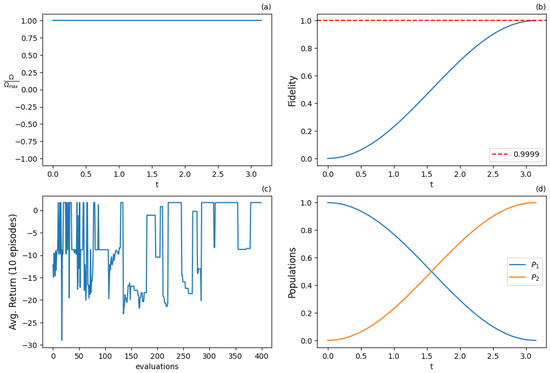
Figure 11.
Results for DQN algorithm with 9 actions and discrete state space after 4000 training iterations: (a) optimal normalized Rabi frequency as control of the system, (b) fidelity (population of excited state |2⟩) as a metric of the population transfer, (c) expected return (cumulative rewards) from the training episodes averaged from 10 episode samples, (d) populations of states |1⟩ and |2⟩. Agent attains the optimal pulse shape for this problem (-pulse).

Table 5.
DQN parameters—hybrid state space.
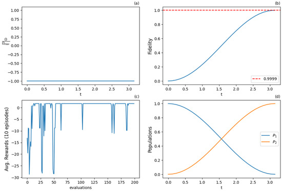
Figure 12.
Results for DQN algorithm with 9 actions and hybrid state space of the form (6) with discrete Rabi frequency and continuous density matrix elements after 2000 training iterations: (a) optimal normalized Rabi frequency , (b) fidelity (population of excited state |2⟩), (c) expected return (cumulative rewards) from the training episodes averaged from 10 episode samples, (d) populations of states |1⟩ and |2⟩. In the hybrid setup, agent succeeds in obtaining optimal solution with faster convergence than in the discrete case.
5.2. Policy Gradient Methods
Policy gradient methods use a different approach than the value-based methods. They parameterize the policy and are trained with simulations to adjust the policy parameters and converge to a local or the global minimum, which produces the optimal policy. In the present work, the models that were used to parameterize the policy were deep neural networks.
REINFORCE with the baseline algorithm uses a critic neural network, representing the parameterized policy, which follows the performance gradient and is step-by-step improved approaching optimal or near-optimal policies. The baseline introduced is a value neural network that estimates the value of the input state. The algorithm was applied for a discrete action space with nine actions and discrete state space configuration (5); see NN architecture 1 in Figure 4a and parameters in Table 6. For a continuous action and state space configuration (6) on resonance (), see NN architecture 2 in Figure 4b and parameters in Table 7. For a continuous action and state space configuration (7) with additional detuning control, the NN architecture in Figure 4b was modified by adding at the input, while the corresponding parameters are given in Table 8. The results are displayed in Figure 13, Figure 14 and Figure 15, respectively. In all the investigated setups, the target fidelity threshold was obtained. In the absence of detuning control, the optimal -pulse is recovered, see Figure 13a and Figure 14a, while in the presence of detuning control, the pulse is approximately obtained, see Figure 15a, with constant and . Among the resonant control configurations, the one with continuous action and state spaces exhibits less variance during training, as shown by comparing Figure 13c and Figure 14c. The addition of detuning control increases the variance during training, see Figure 15c. Note that the extra control variable does not accelerate the population inversion, at least at a noticeable level. The real advantage of using detuning control comes in more complicated situations where there is uncertainty in the qubit frequency or the goal is to manipulate a collection of qubits with different frequencies, problems that are essential for quantum sensing applications. We plan to investigate the power of RL to tackle such complex problems in future work.

Table 6.
REINFORCE with baseline parameters—discrete action and state space.

Table 7.
REINFORCE with baseline parameters—continuous action and state spaces—Resonant case ().

Table 8.
REINFORCE with baseline parameters—continuous action and state spaces—Additional detuning control.
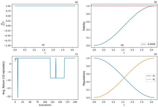
Figure 13.
Results for REINFORCE algorithm with 9 actions and discrete state space after 2000 training iterations: (a) optimal normalized Rabi frequency as the external control, (b) fidelity (population of excited state |2⟩) as the metric of the population transfer, (c) expected return (cumulative rewards) from the training episodes averaged from 10 episode samples, (d) populations of states |1⟩ and |2⟩. Agent succeeds in giving the optimal solution (-pulse).
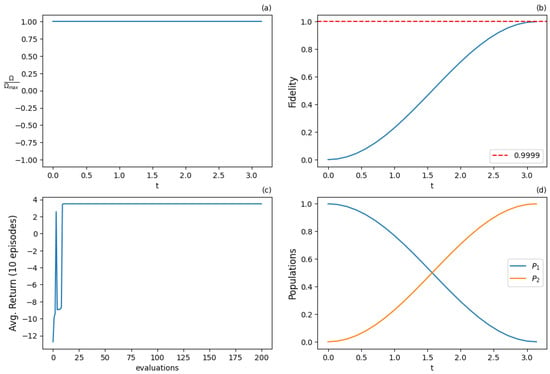
Figure 14.
Results for REINFORCE algorithm with continuous action and state spaces for the resonant case () after 2000 training iterations: (a) optimal normalized Rabi frequency as the external control, (b) fidelity (population of excited state |2⟩) as the metric of the population transfer, (c) expected return (cumulative rewards) from the training episodes averaged from 10 episode samples, (d) populations of states |1⟩ and |2⟩. Optimal -pulse shape is successfully obtained by the training process.
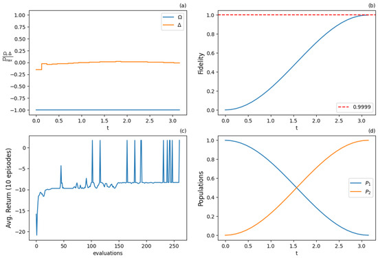
Figure 15.
Results for REINFORCE algorithm with continuous action and state spaces with additional detuning control () after 3000 training iterations: (a) optimal normalized Rabi frequency (blue) and detuning (orange) as two external controls of the system, (b) fidelity (population of excited state |2⟩), (c) expected return (cumulative rewards) from the training episodes averaged from 10 episode samples, (d) populations of states |1⟩ and |2⟩. Agent successfully produces optimal solution that approximates the resonant pulse.
5.3. Actor-Critic Methods
Actor-critic methods try to exploit the advantages of both the value-based and policy gradient methods. The best results are given by the PPO algorithm, which is mostly used with continuous action and state spaces. The algorithm finds successful (near-) optimal policies for both the resonant configuration (Table 9, Figure 16) and the case with additional detuning control (Table 10, Figure 17), obtaining fidelities higher than 0.9999. Note that in the former case, the pulse is recovered, while in the latter case, there is a bang-bang modulation of the detuning between its minimum and maximum allowed values (orange line in Figure 17a), which does not noticeably speed up the population inversion. The addition of detuning control increases the variance during training, as observed by comparing Figure 16c and Figure 17c.

Table 9.
PPO parameters—continuous action and state space—resonant case ().
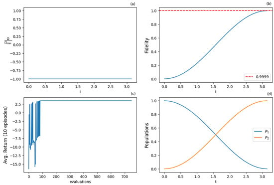
Figure 16.
Results for PPO algorithm with continuous action and state space for the resonant case () after 1500 training iterations: (a) optimal normalized Rabi frequency as the external control, (b) fidelity (population of excited state |2⟩) as the metric of the state transfer, (c) expected return (cumulative rewards) from the training episodes averaged from 10 episode samples, (d) populations of states |1⟩ and |2⟩. Agent successfully solves the problem in the optimal way (-pulse).

Table 10.
PPO parameters—continuous action and state space—additional detuning control.
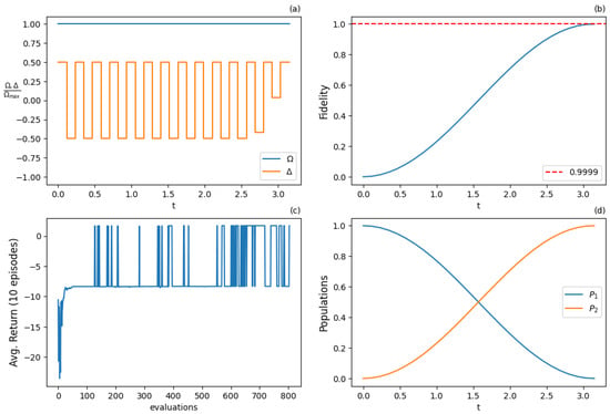
Figure 17.
Results for PPO algorithm with continuous action and state space with additional detuning control () after 2000 training iterations: (a) optimal normalized Rabi frequency and detuning as the two external control functions, (b) fidelity (population of excited state |2⟩) as the metric of the state transfer, (c) expected return (cumulative rewards) from the training episodes averaged from 10 episode samples, (d) populations of states |1⟩ and |2⟩. Agent utilizes both controls to produce an optimal solution.
5.4. Trigonometric Series Optimization Algorithm (TSOA)
The TSOA algorithm can produce a policy that gives the coefficients of the trigonometric series in Equations (29) and (30), so the resultant smooth controls attain the target threshold fidelity of . The parameters of the algorithm are given in Table 11. With a few harmonics and quite small neural networks, the optimization process is able to produce smooth pulses that are (near-)optimal and solve the problem by achieving the desired fidelity, as displayed in Figure 18. The optimal coefficients for the harmonics in Equations (29) and (30) obtained from the optimization are shown in Table 12. Note that the duration of pulses in the TSOA algorithm is fixed a priori, which means that the system is not able to optimize the procedure with respect to timing, but, given a time interval, it is able to obtain optimal smooth pulses attaining the target fidelity, within the algorithm and time discretization limitations.

Table 11.
Parameters for TSOA—PPO algorithm.
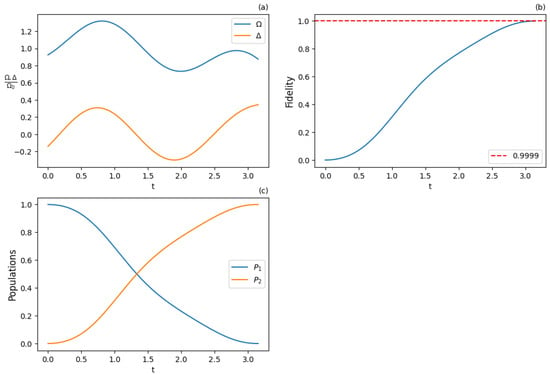
Figure 18.
Results for TSOA—PPO algorithm achieving fidelity of 0.99999: (a) optimal Rabi frequency and detuning , (b) fidelity (population of excited state |2⟩), (c) populations of states |1⟩ and |2⟩. Agent uses a finite trigonometric series function consisting of 3 harmonics to produce a very-high-fidelity solution.

Table 12.
Optimal trigonometric series parameters for fidelity > 0.9999.
6. Conclusions and Future Work
RL methods can provide optimal or suboptimal pulses that can be used to control qubit systems. There are different ways to construct the MDP process, with both finite and infinite dimensional action and state spaces. Each formulation provides a different type of freedom and enables the use of even more RL methods from the finite to the infinite cases. The first and most important step is to clearly define the problem of quantum state transfer mathematically as an MDP. This is the key that unlocks the use of RL methods to solve the problem.
Tabular methods can be used with limited applicability, since they require a lot of training episodes to find optimal pulses that achieve high fidelity. They are not able to achieve the target fidelity (0.9999), as required by quantum computing applications. So, deep RL methods were utilized to solve this problem. They are able to produce optimal or suboptimal pulses more easily than the tabular methods. Their expressivity and generalization properties offer freedom in the state and action spaces definition, allowing even infinite continuous spaces. Infinite state spaces are more intuitive and closer to the state space of the quantum system, while infinite action spaces give more freedom in the choice of controls. Deep RL methods are able to produce policies and pulses within the current requirements and to achieve fidelities up to 0.9999 or higher. As expected, fidelities up or larger than 0.9999 are more difficult to achieve since more time steps are required, leading to larger state spaces. This increase requires more training and larger models to be able to approximate the optimal policies. In most cases, RL methods successfully generate pulses that achieve the desired fidelity.
Temporal difference methods can handle continuous state spaces but not continuous action spaces. If continuity in action space is an important requirement, one should employ policy gradient or actor-critic methods since they can easily work with continuous state and action spaces. This could be important in problems where control functions with limited discrete values are not able to solve the problem with high accuracy. More possible values in action spaces automatically implies bigger search spaces. Consequently, the training process would require more iterations to converge to the optimal policy.
The problem was also formulated as another MDP, using truncated trigonometric series to express the controls. This different setup was solved by approximating the optimization process via the deep RL methods to obtain the optimal coefficients in the series. We called the created algorithm the trigonometric series optimization algorithm (TSOA), which is a step forward from the current state in the literature. The algorithm is able to produce smooth controls achieving fidelity higher than 0.9999, which might be easier to implement experimentally.
Other methodologies may be also exploited for the efficient control of a qubit and quantum systems in general. For example, Ref. [36] proposed a novel architecture of heterogeneous graph neural networks to analyze complex networks, while in Ref. [37], output feedback was combined with machine learning approaches for the optimal control of continuous-time systems. These works addressed complex system identification and control in ways that might inspire robust approaches in the quantum context.
RL methods offer more flexibility than other methods, like optimal control. They can be easily adapted, and it seems straightforward to extend them to quantum systems with three or more energy levels, which are encountered in modern quantum technologies. The main implication of the results is that reinforcement learning methods appear to have the potential to tackle important problems in quantum control. Because of their flexibility, these methods can be easily adjusted for the efficient control of more complex systems, such as systems with more energy levels than a qubit (for example real molecules) as well as the simultaneous control of a collection of qubits with different frequencies. This flexibility allows one to add more controls into the model and, by adjusting the parameters of the model, the same techniques can easily scale and tackle more complex problems. Their formulation is not necessarily physics-informed, which means that they can discover on their own feasible solutions for the dynamics of the system, within reasonable restrictions following the physical laws. Another major challenge is to utilize machine learning models to tackle the noise in quantum systems and obtain robust solutions. We plan to address these interesting problems in future works. Note that as systems become more complex, the hyperparameters of the RL methods should be adapted, and the deep neural networks need to be bigger, so they can approximate more complex models. Any problem that can be formulated as an MDP can be solved with the use of RL algorithms. More systematic analysis is needed when RL methods are applied to other problems, such as quantum error correction [38], quantum gates creation [39], and quantum circuit optimization.
Author Contributions
Conceptualization, E.P.; methodology, D.K.; software, D.K.; validation, D.K., D.S. and E.P.; formal analysis, D.K. and D.S.; investigation, D.K.; data curation, D.K.; writing—original draft preparation, D.K., D.S. and E.P.; writing—review and editing, D.K., D.S. and E.P.; visualization, D.K. and D.S.; supervision, E.P. and D.S.; project administration, D.S. All authors have read and agreed to the published version of the manuscript.
Funding
The work of D.S. was funded by an Empirikion Foundation research grant.
Institutional Review Board Statement
Not applicable.
Informed Consent Statement
Not applicable.
Data Availability Statement
The data presented in this study are available on reasonable request from the corresponding author.
Acknowledgments
We acknowledge Ioannis Thanopulos for useful discussions during the development of this work.
Conflicts of Interest
The authors declare no conflict of interest.
Abbreviations
The following abbreviations are used in this manuscript:
| QC | Quantum Control |
| MDP | Markov Decision Process |
| ML | Machine Learning |
| RL | Reingorcement Learning |
| NN | Neural Network |
| ANN | Artificial Neural Network |
| MC | Monte Carlo |
| TD | Temporal Difference |
| SARSA | State Action Reward State Action |
| DQN | Deep Q-Network |
| TSOA | Trigonometric Series Optimization Algorithm |
| PPO | Proximal Policy Optimization |
| TF | Tensor Flow |
References
- Shore, B.W. Manipulating Quantum Structures Using Laser Pulses; Cambridge University Press: Cambridge, UK, 2011. [Google Scholar]
- Stefanatos, D.; Paspalakis, E. A shortcut tour of quantum control methods for modern quantum technologies. Europhys. Lett. 2021, 132, 60001. [Google Scholar] [CrossRef]
- Vitanov, N.V.; Rangelov, A.A.; Shore, B.W.; Bergmann, K. Stimulated Raman adiabatic passage in physics, chemistry, and beyond. Rev. Mod. Phys. 2017, 89, 015006. [Google Scholar] [CrossRef]
- Guéry-Odelin, D.; Ruschhaupt, A.; Kiely, A.; Torrontegui, E.; Martínez-Garaot, S.; Muga, J.G. Shortcuts to adiabaticity: Concepts, methods, and applications. Rev. Mod. Phys. 2019, 91, 045001. [Google Scholar] [CrossRef]
- Boscain, U.; Sigalotti, M.; Sugny, D. Introduction to the Pontryagin maximum principle for quantum optimal control. PRX Quantum 2021, 2, 030203. [Google Scholar] [CrossRef]
- Goerz, M.; Basilewitsch, D.; Gago-Encinas, F.; Krauss, M.G.; Horn, K.P.; Reich, D.M.; Koch, C. Krotov: A Python implementation of Krotov’s method for quantum optimal control. SciPost Phys. 2019, 7, 080. [Google Scholar] [CrossRef]
- LeCun, Y.; Bengio, Y.; Hinton, G. Deep learning. Nature 2015, 521, 436–444. [Google Scholar] [CrossRef]
- Goodfellow, I.; Bengio, Y.; Courville, A. Deep Learning; MIT Press: Cambridge, MA, USA, 2016. [Google Scholar]
- Silver, D.; Huang, A.; Maddison, C.J.; Guez, A.; Sifre, L.; Van Den Driessche, G.; Schrittwieser, J.; Antonoglou, I.; Panneershelvam, V.; Lanctot, M.; et al. Mastering the game of Go with deep neural networks and tree search. Nature 2016, 529, 484–489. [Google Scholar] [CrossRef]
- Krenn, M.; Landgraf, J.; Foesel, T.; Marquardt, F. Artificial intelligence and machine learning for quantum technologies. Phys. Rev. A 2023, 107, 010101. [Google Scholar] [CrossRef]
- Dawid, A.; Arnold, J.; Requena, B.; Gresch, A.; Płodzień, M.; Donatella, K.; Nicoli, K.A.; Stornati, P.; Koch, R.; Büttner, M.; et al. Modern applications of machine learning in quantum sciences. arXiv 2022, arXiv:2204.04198. [Google Scholar]
- Couturier, R.; Dionis, E.; Guérin, S.; Guyeux, C.; Sugny, D. Characterization of a driven two-level quantum system by Supervised Learning. Entropy 2023, 25, 446. [Google Scholar] [CrossRef]
- Bonizzoni, C.; Tincani, M.; Santanni, F.; Affronte, M. Machine-Learning-Assisted Manipulation and Readout of Molecular Spin Qubits. Phys. Rev. Appl. 2022, 18, 064074. [Google Scholar] [CrossRef]
- Sutton, R.S.; Barto, A.G. Reinforcement Learning: An Introduction; MIT Press: Cambridge, MA, USA, 2018. [Google Scholar]
- Bukov, M.; Day, A.G.; Sels, D.; Weinberg, P.; Polkovnikov, A.; Mehta, P. Reinforcement learning in different phases of quantum control. Phys. Rev. X 2018, 8, 031086. [Google Scholar] [CrossRef]
- Giannelli, L.; Sgroi, P.; Brown, J.; Paraoanu, G.S.; Paternostro, M.; Paladino, E.; Falci, G. A tutorial on optimal control and reinforcement learning methods for quantum technologies. Phys. Lett. A 2022, 434, 128054. [Google Scholar] [CrossRef]
- Sivak, V.; Eickbusch, A.; Liu, H.; Royer, B.; Tsioutsios, I.; Devoret, M. Model-free quantum control with reinforcement learning. Phys. Rev. X 2022, 12, 011059. [Google Scholar] [CrossRef]
- Niu, M.Y.; Boixo, S.; Smelyanskiy, V.N.; Neven, H. Universal quantum control through deep reinforcement learning. Npj Quantum Inf. 2019, 5, 33. [Google Scholar] [CrossRef]
- Ding, Y.; Ban, Y.; Martín-Guerrero, J.D.; Solano, E.; Casanova, J.; Chen, X. Breaking adiabatic quantum control with deep learning. Phys. Rev. A 2021, 103, L040401. [Google Scholar] [CrossRef]
- Porotti, R.; Tamascelli, D.; Restelli, M.; Prati, E. Coherent transport of quantum states by deep reinforcement learning. Commun. Phys. 2019, 2, 61. [Google Scholar] [CrossRef]
- Paparelle, I.; Moro, L.; Prati, E. Digitally stimulated Raman passage by deep reinforcement learning. Phys. Lett. A 2020, 384, 126266. [Google Scholar] [CrossRef]
- Brown, J.; Sgroi, P.; Giannelli, L.; Paraoanu, G.S.; Paladino, E.; Falci, G.; Paternostro, M.; Ferraro, A. Reinforcement learning-enhanced protocols for coherent population-transfer in three-level quantum systems. New J. Phys. 2021, 23, 093035. [Google Scholar] [CrossRef]
- An, Z.; Song, H.J.; He, Q.K.; Zhou, D. Quantum optimal control of multilevel dissipative quantum systems with reinforcement learning. Phys. Rev. A 2021, 103, 012404. [Google Scholar] [CrossRef]
- Liu, W.; Wang, B.; Fan, J.; Ge, Y.; Zidan, M. A quantum system control method based on enhanced reinforcement learning. Soft Comput. 2022, 26, 6567–6575. [Google Scholar] [CrossRef]
- Watkins, C.J.; Dayan, P. Q-learning. Mach. Learn. 1992, 8, 279–292. [Google Scholar] [CrossRef]
- Mnih, V.; Kavukcuoglu, K.; Silver, D.; Rusu, A.A.; Veness, J.; Bellemare, M.G.; Graves, A.; Riedmiller, M.; Fidjeland, A.K.; Ostrovski, G.; et al. Human-level control through deep reinforcement learning. Nature 2015, 518, 529–533. [Google Scholar] [CrossRef]
- Williams, R.J. Simple statistical gradient-following algorithms for connectionist reinforcement learning. Mach. Learn. 1992, 8, 229–256. [Google Scholar] [CrossRef]
- Konda, V.; Tsitsiklis, J. Actor-critic algorithms. Adv. Neural Inf. Process. Syst. 1999, 12, 1008–1014. [Google Scholar]
- Grondman, I.; Busoniu, L.; Lopes, G.A.; Babuska, R. A survey of actor-critic reinforcement learning: Standard and natural policy gradients. IEEE Trans. Syst. Man Cybern. Part C Appl. Rev. 2012, 42, 1291–1307. [Google Scholar] [CrossRef]
- Schulman, J.; Wolski, F.; Dhariwal, P.; Radford, A.; Klimov, O. Proximal policy optimization algorithms. arXiv 2017, arXiv:1707.06347. [Google Scholar]
- Schulman, J.; Levine, S.; Abbeel, P.; Jordan, M.; Moritz, P. Trust region policy optimization. In Proceedings of the International Conference on Machine Learning, Lille, France, 6–11 July 2015; pp. 1889–1897. [Google Scholar]
- Stefanatos, D.; Paspalakis, E. Efficient generation of the triplet Bell state between coupled spins using transitionless quantum driving and optimal control. Phys. Rev. A 2019, 99, 022327. [Google Scholar] [CrossRef]
- Martinis, J.M.; Geller, M.R. Fast adiabatic qubit gates using only σ z control. Phys. Rev. A 2014, 90, 022307. [Google Scholar] [CrossRef]
- Abadi, M.; Agarwal, A.; Barham, P.; Brevdo, E.; Chen, Z.; Citro, C.; Corrado, G.S.; Davis, A.; Dean, J.; Devin, M.; et al. TensorFlow: Large-Scale Machine Learning on Heterogeneous Systems. 2015. Available online: https://www.tensorflow.org/ (accessed on 1 April 2024).
- Johansson, J.; Nation, P.; Nori, F. QuTiP 2: A Python framework for the dynamics of open quantum systems. Comput. Phys. Commun. 2013, 184, 1234–1240. [Google Scholar] [CrossRef]
- Wang, Y.; Liu, Z.; Xu, J.; Yan, W. Heterogeneous network representation learning approach for ethereum identity identification. IEEE Trans. Comput. Soc. Syst. 2022, 10, 890–899. [Google Scholar] [CrossRef]
- Zhao, J.; Lv, Y.; Zeng, Q.; Wan, L. Online Policy Learning Based Output-Feedback Optimal Control of Continuous-Time Systems. IEEE Trans. Circuits Syst. II Express Briefs 2022, 71, 652–656. [Google Scholar] [CrossRef]
- Fösel, T.; Tighineanu, P.; Weiss, T.; Marquardt, F. Reinforcement learning with neural networks for quantum feedback. Phys. Rev. X 2018, 8, 031084. [Google Scholar] [CrossRef]
- An, Z.; Zhou, D. Deep reinforcement learning for quantum gate control. Europhys. Lett. 2019, 126, 60002. [Google Scholar] [CrossRef]
Disclaimer/Publisher’s Note: The statements, opinions and data contained in all publications are solely those of the individual author(s) and contributor(s) and not of MDPI and/or the editor(s). MDPI and/or the editor(s) disclaim responsibility for any injury to people or property resulting from any ideas, methods, instructions or products referred to in the content. |
© 2024 by the authors. Licensee MDPI, Basel, Switzerland. This article is an open access article distributed under the terms and conditions of the Creative Commons Attribution (CC BY) license (https://creativecommons.org/licenses/by/4.0/).