A Comparative Analysis of the Bayesian Regularization and Levenberg–Marquardt Training Algorithms in Neural Networks for Small Datasets: A Metrics Prediction of Neolithic Laminar Artefacts

Abstract

This study aims to present a comparative analysis of the Bayesian regularization backpropagation and Levenberg–Marquardt training algorithms in neural networks for the metrics prediction of damaged archaeological artifacts, of which the state of conservation is often fragmented due to different reasons, such as ritual, use wear, or post-depositional processes. The archaeological artifacts, specifically laminar blanks (so-called blades), come from different sites located in the Southern Levant that belong to the Pre-Pottery B Neolithic (PPNB) (10,100/9500–400 cal B.P.). This paper shows the entire procedure of the analysis, from its normalization of the dataset to its comparative analysis and overfitting problem resolution.

1. Introduction

Artificial intelligence (AI), specifically both machine learning (ML) and deep learning (DL), has lately been applied to archaeology in several ways, such as for the identification of sites’ locations, their extensions, archaeological artifacts’ dispersion in sites [1,2,3,4,5,6], as well as for taxonomic/typological artifact identification [7,8,9].

The application of these methodologies has great potential due to the nature of the archaeological artifacts and their typological and technological variety, which influence the potential parameters and variables to be considered depending on the study case, to which we need to add the several possibilities that AI provides us in terms of the variety of algorithms depending on the analysis.

In this study, we proposed a deep-learning comparative analysis based on a feedforward neural network based upon the Bayesian and Levenberg–Marquardt training regularization algorithms for the metrics prediction of damaged regular artifacts, or rather of laminar blanks (so-called blades), collected from the PPNB sites of Nahal Ruel, Yiftahel and Motza.

This research aimed to define a standard procedure for an archaeological application of neural networks in metrics prediction, highlighting the advantages and disadvantages by using the Bayesian regularization backpropagation [10,11] or the Levenberg–Marquardt [12,13] training algorithms on a small database, showing its normalization process, solutions for underfitting and overfitting issues, and differences concerning the training process, error span, and results.

2. Material and Methods

The materials selected for this analysis were debitage artifacts, specifically blades and bladelets. The selection was made using a random-stratified methodology, which allowed the selection of any technological subcategories in which these laminar blanks are divided [14,15]. These artifacts are known in archaeology to be the most regular artifacts in terms of the dimensional proportion and technology. The realization of these elements is indeed obtainable through a pre-determined reduction process of the raw material (in this case, flint), mostly based on bidirectional and secondarily unidirectional technology [16,17]. These artifacts belong to the technological category of laminar blanks, which can be further divided into two sub-categories: blades and bladelets. Both represent elongated artifacts with a length of at least twice their width. Bladelets are artifacts with a length smaller than 50 mm and a width narrower or equal to 12 mm, while blades are artifacts with a length longer than 50 mm and a width larger than 12 mm.

The measuring method used for obtaining dimensional information on each artifact was based on measuring the maximum technological length, width, and thickness, and if it was possible due to the state of conservation, the thickness and width were measured in specific positions according to the technological characteristics of any lithic artifacts, which are represented by the localization of the proximal and distal ends. The width and thickness were indeed also measured on the line that separates the proximal end and mesial part, and on the line that separates the mesial part and the distal end (Figure 1). This methodology allowed us to obtain all the possible information, not only on undamaged artifacts but also on fragmented ones (Figure 2).

Due to the state of conservation of the artifacts and the most suitable amount for a proper neural network, we decided to focus the comparative analysis on the metrics prediction of artifacts of which the distal end has not been preserved, either due to use wear, re-shaping, or ritual processes. For this study, a total of 291 artifacts were used. Out of these, 181 laminar artifacts that were undamaged were used as input. These 181 artifacts were further sub-divided into 149 blades and 32 bladelets. The remaining 110 laminar artifacts that had a missing distal end were used as output. These 110 artifacts were further sub-divided into 85 blades and 35 bladelets.

Concerning the application of AI to the materials, an ML method was chosen as the most relevant method available for this analysis. Both the Bayesian regularization backpropagation (BRBP) and Levenberg–Marquardt training algorithms were chosen to obtain the most performant results on a small set of data [18,19].

In Bayesian regularization backpropagation learning algorithms, the objective function is the mean square error. The mean square error (MSE) measures the average squared difference between the predictions and the actual targets:

$$\mathit{MSE}=\frac{1}{n}{\sum }_{i=1}^n(Y_i-y_i{)}^2=\frac{1}{n}{\sum }_{i=1}^n{e}_i^2$$

where:

$n$ is the number of elements in the dataset.

$y$ is the neural network output.

$Y$ is the target output corresponding to $y$.

In the BRBP algorithm, the objective function is as follows:

$$F\left(\omega \right)=\alpha E_{\omega }+\beta E_D$$

where:

$\alpha \mathrm{a}\mathrm{n}\mathrm{d} \beta$ represent two regularization coefficients.

ω represents the neural network weights.

$E_{\omega }$=$\sum _i{\omega }_i^2$ represents the sum of the squared network weight and $E_D$ is the data error term.

Including E_ω in the objective function alongside the data error term $E_D$ allows the algorithm to find a balance between fitting the training data well (minimizing $E_D$) and keeping the model’s complexity in check (minimizing E_ω).

The objective function used in the BRBP algorithm is responsible for guiding the training of the neural network. This function is comprised of two main components. The first component minimizes the sum of the squares of the network weights, while the second component (e) represents the error between the model’s predictions and the actual data or targets. The objective of this function is to ensure that the model is making accurate predictions on the training data, thus resulting in a well-trained neural network.

The coefficients α and β control the influence of each term on the overall objective.

The process of finding the optimum values for α and β in the context of Bayesian regularization can indeed be challenging. These parameters play a crucial role in balancing the trade-off between fitting the training data well and controlling the complexity of the model.

The statement suggests that the relative values of α and $\beta$ influence the training error differently. Specifically:

If $\alpha \ll \beta$, smaller values of α compared to $\beta$ lead to smaller errors related to the regularization term on the sum of the squared network weights E_ω. This means that the algorithm may prioritize fitting the training data more closely, potentially risking overfitting if not properly controlled.

If $\alpha \gg \beta$, larger values of $\alpha$ compared to $\beta$ emphasize the importance of reducing the size of the network weights. This encourages the algorithm to prefer simpler models with smaller weights, even if it comes at the cost of slightly higher errors in the training data.

To determine the optimal values for $\alpha$ and $\beta$, we used a Bayesian regularization method. Bayesian methods usually involve introducing prior distributions of the parameters (in this case, ω), updating these distributions with observed data, and then making probabilistic inferences. In the regularization system, this approach allows for a principled way of incorporating uncertainty and making informed decisions about the balance between fitting the data and controlling the model complexity. The Bayesian regularization method is based on Bayes’ theorem in the following way:

$$P\left(\left.A\right|B\right)=\frac{P\left(\left.B\right|A\right)\cdot P\left(A\right)}{P\left(B\right)}$$

where:

$P\left(\left.A\right|B\right)$ is the posterior probability of event A, given B.

$P\left(\left.B\right|A\right)$ is the prior probability of event B, given A.

$P\left(A\right)$ is the prior probability of event A.

$P\left(B\right)$ is the non-zero prior probability of event B, serving as a normalizing constant.

Bayes’ theorem provides a mathematical framework for updating our prior beliefs in light of new evidence. It enables us to refine our initial assumptions by incorporating observed data, resulting in a more accurate and reliable estimate of the underlying probability distribution. By applying Bayes’ theorem, we can determine the posterior probability of a hypothesis, given our prior belief and the likelihood of observing the available evidence.

In order to find the optimal weight space in the Bayesian framework, the objective function F(ω) needs to be minimized to make it equivalent to maximizing the posterior probability function as follows:

$$P(\omega |D,\alpha ,\beta ,M)=\frac{P\left(D\right| \omega ,\beta ,M\left)P\right(\omega |\alpha ,M)}{P\left(D\right|\alpha ,\beta ,M)}$$

where:

D stands for the dataset.

M is the specific neural network model being used.

$\omega$ is the vector of the network weights.

P(ω|α,M) is the prior density. It encapsulates our prior knowledge about the weights ω before we have observed any data.

This is a fundamental concept in Bayesian statistics, where our prior beliefs are updated as far as new data are added. In a neural network model M, the prior knowledge could be either based on previous studies, expert knowledge, or other relevant information.

$P\left(D\right| \omega ,\beta ,M)$ is the likelihood function. It represents the observation probability of data D, given the weights ω, under the specific model M. It quantifies how well the selected model is, while the specific set of weights explains the observed data. In other words, if you were to use the model M with weights ω to generate data, the likelihood function tells you the probability that the model would generate the observed data D. It is a fundamental concept in machine learning and statistics that helps us understand how well our model represents the data we have.

P(D|α,β,M) represents a normalization factor in this context. In Bayesian inference, the posterior distribution of the parameters is often a priority, because it is proportional to the likelihood and the prior product. However, to ensure that the posterior distribution is a valid probability distribution, it is necessary to ensure that it integrates (or sums) to 1 over all the possible values of the parameters. This is the exact step where the function P(D|α,β,M) comes in. It essentially represents the integral (or sum) of the product of the likelihood and the prior overall possible values of the parameters. By using this system, the posterior distribution is guaranteed to be a valid probability distribution that adds up to 1. This term is often difficult to calculate directly, especially for complex models and large datasets, but various computational techniques, such as Markov chain Monte Carlo (MCMC), are often used to handle this.

Bayesian regularization in backpropagation algorithms typically involves incorporating prior distributions over the model parameters and updating them using techniques such as variational inference or Markov Chain Monte Carlo (MCMC) methods. The steps in a Bayesian regularization backpropagation algorithm would generally involve the following:

Initialization: Initialization of the weights and biases of the neural network.

Forward Pass: Performance of a forward pass through the network to compute the predicted output for a given input.

Compute Loss: Calculation of the loss function, which is typically a combination of a data term (e.g., mean squared error) and a regularization term based on the prior distribution over the model parameters.

Backward Pass (Backpropagation): A backpropagation approach to compute the gradients of the loss function in relation to the model parameters.

Update Parameters: Update the model parameters using both the gradients achieved in the previous step and an optimization algorithm such as the stochastic gradient descent (SGD) or its variants.

Incorporate Bayesian regularization as follows:

Prior Specification: Definition of prior distributions over the model parameters, which may include Gaussian priors, Laplace priors, etc.

Variational Inference or MCMC Sampling: Performance of variational inference or MCMC sampling to approximate the posterior distribution over the model parameters, given the observed data and the prior distributions.

Update Parameters with Regularization: Update the model parameters using the gradients achieved from the posterior distribution, incorporating the Bayesian regularization term into the update rule.

Repetition: Repetition of steps 2–6 for a specified number of iterations or until the convergence criteria are met.

Prediction: After training, the trained model must be used for making predictions on new data by performing a forward pass through the network.

Evaluation: Evaluation of the performance of the trained model on a separate validation or test dataset using appropriate metrics. The specifics of the implementation of this algorithm may vary depending on the choice of prior distributions and inference techniques.

The Levenberg–Marquardt training algorithm is instead aimed at minimizing a cost function, defined as the residual sum of squares (RSS). This cost function is used in nonlinear regression problems and the optimization of models. Furthermore, the model parameters are iteratively updated using a combination of descending gradient methods and Newton methods, exemplified by the following formula:

w_k+1 = w_k − (J_k^TJ_k + μ _I)⁻¹J_k e_k

where:

w_k+1 = w_k − αg_krepresents the EPB algorithm

w_k+1 = w_k − H_k⁻¹g_k is the Newton algorithm

w_k+1 = w_k− (J_k^TJ_k)⁻¹J_ke_k is the Newton–Gauss algorithm

The EPB algorithm, the Newton–Gauss algorithm, and the Newton algorithm are methods used to optimize the parameters in different types of problems.

The EPB algorithm is commonly used in machine learning to optimize the parameters in learning classifiers or regressors. It works by iteratively minimizing an objective function (or loss) with a gradient descent-based approach. The learning rate may vary during optimization, and an exponential term may be included to boost or penalize the objective function based on its current value.

The Newton–Gauss algorithm, also known as Gauss–Newton, is used in nonlinear regression problems to optimize the parameters. It updates the parameters using an approximate version of the Hessian matrix, which is the matrix of second derivatives of the objective function with respect to the parameters. The Newton–Gauss algorithm is particularly useful when the objective function is approximately quadratic near the minimum.

The Newton algorithm is an optimization method commonly used to solve nonlinear optimization problems. It uses the second derivative of the objective function to guide the parameter updates and can converge more quickly than other optimization methods, especially when the objective function is convex and well-behaved. However, it may require computationally expensive calculations of the Hessian matrix and may not be stable in all situations.

During each iteration, the algorithm balances between Newton’s steps and the gradient steps, using an “amortization” parameter to control the step size, which helps to avoid divergence or slowness issues. The algorithm iteratively continues to update the parameters until convergence is reached or until a stop criterion is fulfilled.

During the training process of the neural network, several parameters were custom-made and set in MATLAB. Each parameter has a specific role in the neural network training process. Here is an explanation of each parameter:

• net.trainParam.epochs: This parameter specifies the number of epochs, which is the number of times the entire training set is presented to the neural network for training. A complete era is when the network has seen and learned from all the training data once.
• net.trainParam.lr: This parameter represents the learning rate (LR). It indicates how many times the neural network should update the weights based on the error during each iteration of the optimization algorithm. A higher learning rate may accelerate the training, but it may also cause oscillations or converging difficulties.
• net.trainParam.max_fail: This parameter represents the maximum number of consecutive failures allowed during training. If the network error stops decreasing for several epochs specified by this parameter, the training may stop before reaching the maximum number of epochs to avoid overfitting problems.
• net.trainParam.min_grad: This parameter specifies the minimum gradient threshold. During training, if the weight gradient of the neural network becomes lower than this value, the optimization algorithm may consider that the network has reached a convergence condition.
• net.trainParam.goal: This parameter is the training performance goal. It represents the average error that you want to achieve during training. Once the average neural network error reaches or approaches this value, the training ends.

The parameters chosen are heavily dependent on the specific problem confronted, the complexity of the dataset, and the structure of the neural network. However, there are some suggested best practices to be considered, such as the following:

• The learning rate (LR) should be initially set to small values and then adjusted as the training proceeds to avoid oscillations and divergence.
• The number of epochs (epochs) should be sufficient to allow the network to learn from the data, but not too large to avoid overfitting.
• max_fail can be adjusted according to the training stability and overfitting measurement.
• min_grad and goal are often set according to the desired accuracy and tolerance for convergence.

In both cases, the neural network was built on two hidden layers: 1 composed of 80 perceptrons and 1 composed of 40 perceptrons. This specific architecture was chosen after several tests set on different amounts of perceptrons in order, first, to avoid underfitting problems due to the low number of artifacts (small dataset), and secondly, to achieve the best results and to avoid overfitting problems.

The input layer therefore consisted of four perceptrons, as many as the known variables for every single artifact, such as the length, mesial width, and mesial thickness; two hidden layers; and one output layer represented by three perceptrons, as many as the number of unknown variables, comprising the missing metric information to be predicted by the neural network (Figure 3).

where:

$x_j^k$ represents the output of the j-th node located on the K-layer;

$x_i^{k-1}$ is the output of the i-th node on the K-1-layer;

${\omega }_{i,j}^k$ is the connection weight between nodes $i$ and j.

The node activation function (perceptron) is as follows (Figure 4):

$$R\left(s\right)=\frac{1}{1+e^{-s}}$$

(1)

Taking Equation (1) as the node activation function (perceptron), it can be formulated in the following way:

$$x_j^{\left(k\right)}=R({\sum }_{i=0}^M{\omega }_{i,j}^{\left(k\right)}{x}_i^{(k-1)}+b_i^{\left(k\right)})$$

(2)

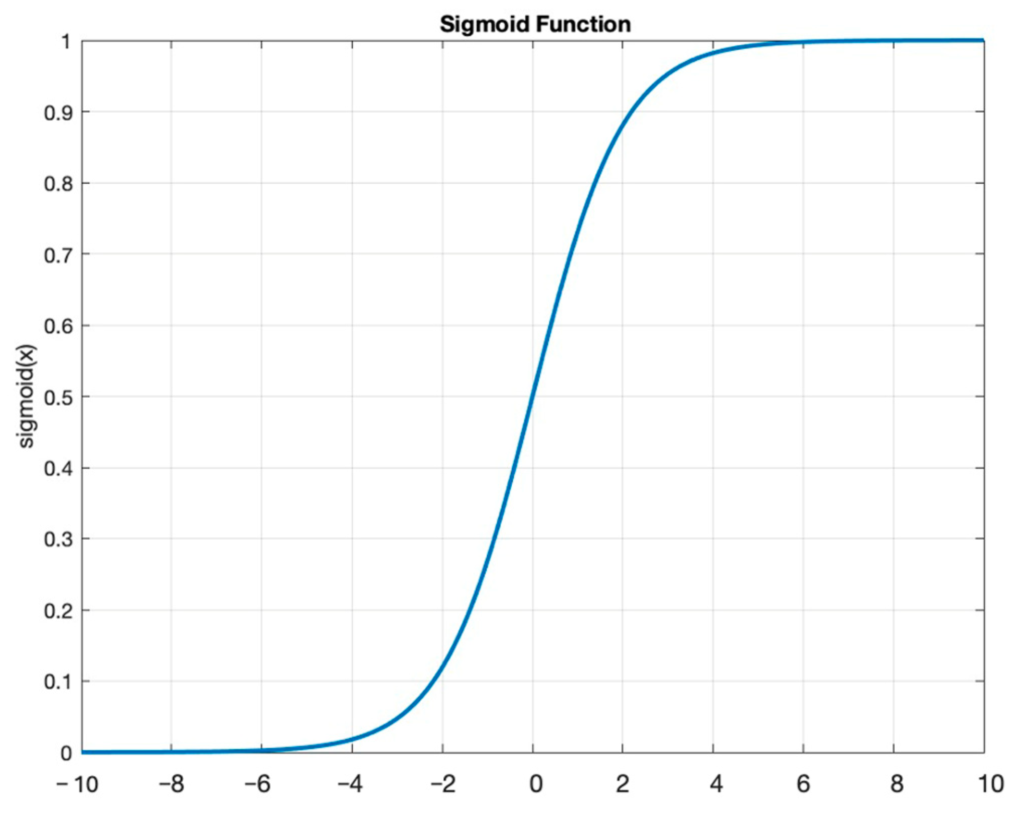
Concerning the activation function of the perceptrons, two different functions were selected. One activation function corresponded to the sigmoid not-tangent hyperbolic and was meant to be used for the hidden layers, and the other activation function corresponded to a linear function and was meant to be used for the last output layer. The choice of activation functions for the neural network layers is crucial because it affects the network’s ability to learn and represent complex data relationships. We ultimately settled on this specific activation function, which produced the desired outcomes. The hidden layer activation function was the sigmoid not-tangent hyperbolic function (Figure 5), which is commonly used in neural network studies to introduce non-linearities and represents the best solution for the purpose of this study. A linear function was instead used for the output layer.

In neural networks, the error E is defined by the difference between the expected vector and the real value.

$$E=\frac{1}{2}{{\sum }_{j=1}^{M_K}(x_j^{\left(k\right)}-{d_j}^{\left(k\right)})}^2$$

(3)

where:

d_j defines the expected error;

$x_j^{\left(k\right)}$ represents the real output value at node j;

$M_K$ defines the number of nodes in the K-th layer.

The aim is to achieve an approach between the output values’ vector and the expected values’ vector. Therefore, it is possible to minimize Equation (3) by adjusting the values of weights ${\omega }_{i,j}$ among the serval nodes, allowing us to consider the derivative of (3) as follows:

$$\frac{\partial E}{{{\partial \omega }^{\left(K\right)}}_{i,j}}=\left(x_j^{\left(k\right)}-{d_j}^{\left(k\right)}\right)\frac{\partial x_j^{\left(k\right)}}{\partial {\omega }_{i,j}^{\left(k\right)}}$$

(4)

$$\frac{\partial x_j^{\left(k\right)}}{\partial {\omega }_{i,j}^{\left(k\right)}}=\frac{\partial }{\partial {\omega }_{i,j}^{\left(k\right)}}R({\sum }_{i=0}^{M_{K-1}}{\omega }_{i,j}^{\left(k\right)}{x}_i^{(k-1)}+b_i^{\left(k\right)})$$

(5)

By choosing R(s) as the function achieved in Equation (1), its derivative will be:

$$\frac{\partial R\left(s\right)}{\partial s}=R\left(s\right)\left[1-R\left(s\right)\right]$$

(6)

Applying (6) to (5), the following function is obtained:

$$\frac{\partial x_j^{\left(k\right)}}{\partial {\omega }_{i,j}^{\left(k\right)}}=x_j^{\left(k\right)}\left(1-x_j^{\left(k\right)}\right).x_i^{\left(k-1\right)}$$

(7)

Substituting (7) into (4), the following function is achieved:

$$\frac{\partial E}{\partial {{\omega }^{\left(K\right)}}_{i,j}}=\left(x_j^{\left(k\right)}-{d_j}^{\left(k\right)}\right)x_j^{\left(k\right)}\left(1-x_j^{\left(k\right)}\right).x_i^{\left(k-1\right)}$$

(8)

The following equation shows that changing the weights ${\omega }_{i,j}$ is sufficient to minimize the error by starting from random values for the various weights at time t = 0, w_(i,j):

$${\omega }_{i,j}^{\left(k\right)}\left(t+1\right)={\omega }_{i,j}^{\left(k\right)}\left(t\right)-\eta \frac{\partial E}{\partial {{\omega }_{\left(K\right)}}_{i,j}}$$

(9)

where:

η defines the learning rate that assumes a value range from 0.1 to 0.9. It represents the value that adjusts the algorithm learning rate.

Starting from the iteration at instant t = 0 in the next one t + 1, it is necessary to adjust the weights until (9) converges.

Substituting (8) into (9), the following function is achieved:

$${\omega }_{i,j}^{\left(k\right)}\left(t+1\right)={\omega }_{i,j}^{\left(k\right)}\left(t\right)-\eta \left(x_j^{\left(k\right)}-d_j\right)x_j^{\left(k\right)}\left(1-x_j^{\left(k\right)}\right).x_i^{\left(k-1\right)}$$

(10)

Therefore:

$${\delta }_j^{\left(k\right)}=\left(x_j^{\left(k\right)}-d_j\right)x_j^{\left(k\right)}\left(1-x_j^{\left(k\right)}\right)$$

(11)

In conclusion, rewriting the function (10):

$${\omega }_{i,j}^{\left(k\right)}\left(t+1\right)={\omega }_{i,j}^{\left(k\right)}\left(t\right)-\eta {\delta }_j^{\left(k\right)}{x}_i^{\left(k-1\right)}$$

(12)

Based on these considerations, a feedforward backpropagation learning algorithm can be implemented by applying the following operations:

Random initialization of weights ${\omega }_{i,j}^{\left(k\right)}$; the network input vector is set to “target” samples with which a vector of the output values is necessary to classify the model correctly.

The function needs to be calculated for each layer from the input to the output as follows:

$$x_j^{(k+1)}=R({\sum }_{i=0}^{M_K}{\omega }_{i,j}^{(k+1)}{x}_i^{\left(k\right)}+b_i^{\left(k\right)})\hspace{1em}\hspace{1em}k=0,\dots ,\left(k-1\right),j=1,\dots {, M}_{K+1}$$

For each node, calculate the following function starting from the output layer:

$${\delta }_j^{\left(k\right)}=\left(x_j^{\left(k\right)}-d_j\right)x_j^{\left(k\right)}\left(1-x_j^{\left(k\right)}\right)\hspace{1em}\hspace{1em}\hspace{1em}\hspace{1em}\hspace{1em}\hspace{1em}j=1,\dots ,M_K$$

For hidden layers ranging from (k − 1) to 1, the calculation is as follows:

$${\delta }_j^{\left(k\right)}=x_j^{\left(k\right)}\left(1-x_j^{\left(k\right)}\right)\sum _{j=1}^{M_{K+1}}{\delta }_j^{(k+1)}{\omega }_{i,j}^{(k+1)}$$

Update of weight values as follows:

$${\omega }_{i,j}^{\left(k\right)}\left(t+1\right)={\omega }_{i,j}^{\left(k\right)}\left(t\right)-\eta {\delta }_j^{\left(k\right)}{x}_i^{\left(k-1\right)}$$

Repetition of the previous steps is performed until the convergence is achieved.

If the mean square error increases as the weights increase $\frac{\partial E}{\partial {{{{\omega }^{\left(K\right)}}^{ }}_{i,j}}^{ }}>$0, the algorithm predicts a decrease in the weights $∆{{{{\omega }^{\left(K\right)}}^{ }}_{i,j}}^{ }<0$; otherwise, if the error decreases as the weights increase, the backpropagation learning algorithm then has high convergence times and may stop at a local minimum. It is possible, therefore, to analyze other algorithms that provide solutions to these problems and that are part of the backpropagation group but differ from the classical algorithm by the method used to update the weights.

Taking into account the Newton’s algorithm, the weights are updated according to the following law:

$$W\left(t+1\right)=W\left(t\right)-H^{-1}\left(t\right)g\left(t\right)$$

(13)

where:

$W$ is the matrix of the weights;

H is the Hessian matrix of the error;

g is the gradient of the error.

To improve the accuracy of a model, it is necessary to update the weights and biases of the model through multiple iterations. However, this process involves the computation of the Hessian matrix, which is the matrix of the second derivatives of the error with respect to the weights. This computation can be quite onerous.

Luckily, there is a class of algorithms called quasi-Newton algorithms that can make this process much simpler. One such algorithm is the Levenberg–Marquardt algorithm. This algorithm does not require the computation of the Hessian matrix. Instead, it approximates the Hessian matrix and error gradient using equations that are much easier to compute, as shown in (14) and (15):

$$H=J^{T}J$$

(14)

$$g=J^{T}E$$

(15)

where:

J is the Jacobian matrix whose elements are the prime derivatives of the error with respect to the weights;

E is the error vector.

If functions (14) and (15) are merged into (13), then the update matrix of the weights becomes as follows:

$$W\left(t+1\right)=W\left(t\right)-{\left[J^{T}J\right]}^{-1}{J}^{T}E$$

(16)

The latter algorithm (16) was chosen to perform the neural network learning ability. The generalization of the network is the ability to recognize data that are slightly different from the data it was trained with. Too much data in the learning phase might affect the network on the training set, causing overfitting problems, and thus it might limit the ability to generalize. A few data may instead not be enough to reduce the overall error; therefore, it is indispensable to understand when it is necessary to stop training the network in order not to incur learning data overfitting. A method to optimize the generalization ability is the “early stopping” method.

The training data were randomly divided into two subsets. The larger subset was used for the training, where the network’s weights must be necessarily adjusted, while the smaller subset was reserved for testing. The validation test was performed by selecting from the training dataset a subset called “validation set”. During the training algorithm, the error trend was periodically tested with the validation set. When it started increasing, the training was stopped. Subsequently, it was fundamental to verify the final accuracy in terms of correct answers (expressed in percentages) compared to the test set data. It might be plausible to think, observing the error trend, that it could decrease proportionally to the increase in the weights’ update. It is essential to avoid continuing the training process beyond the point where the validation error is as low as possible, as this can cause the network to only learn the “noise” present in the training set. A good network is considered to generate an error of less than 20% of the input/output pairs on the final test.

Finally, for neural network learning, a database of exclusively complete and undamaged artifacts was used. A total of 70% of the undamaged artifacts in each prediction were used for the training process, and the remaining 30% were used for the error calculation. Furthermore, both the algorithms divided the 70% into three sets: one for the proper training process, one for the data validation, and one for the final test. In both the training and validation processes, the selection was random, with no experimenter decisions or interference that might have affected the results (Supplementary Material S1).

The neural networks were tested with different LRs for both the Bayesian (LR_Ba) and Levenberg–Marquardt (LR_LM) regularization training algorithms, respectively, set as LR_{Ba_1} = 0.1; LR_{Ba_2} = 0.3; LR_{Ba_3} = 0.4; LR_{LM_!} = 0.1; LR_{LM_2} = 0.3; LR_{LM_3} = 0.4.

Therefore, a comparative analysis was conducted for each test at the same rate.

3. Results

The neural network procedure usually requires setting an initially low learning rate. As the training progresses, adjustments are made to prevent oscillations and divergence. For this reason, the results are shown gradually.

3.1. Bayesian vs. Levenberg–Marquardt Based on LR = 0.1

The LR = 0.1 test showed a low capability for the metrics prediction, with a higher error that even led to negative values, which should be impossible for the artefacts’ dimensions due to the inexistence per se of negative metrics. The Bayesian training regularization algorithm and the Levenberg–Marquardt algorithm produced similar results.

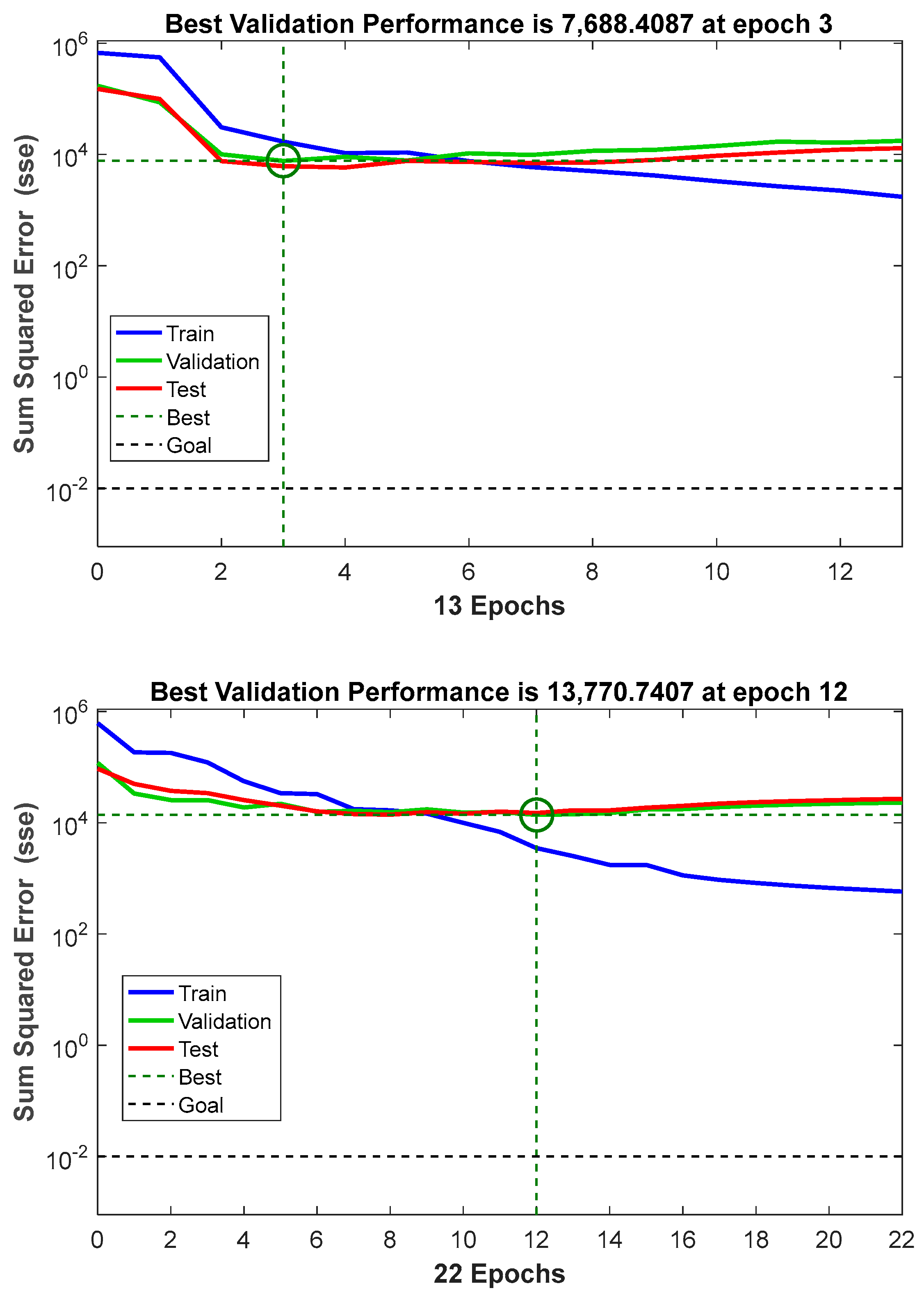
The Bayesian regularization algorithm using an LR set on 0.1 achieved the best validation performance of 7688.4087 at epoch 3 and stopped at epoch 13. The Levenberg–Marquardt algorithm, also using the same LR as the previous algorithm, achieved the best validation performance of 13,770.7407 at epoch 12 and stopped at epoch 22 (Figure 6).

The errors were calculated according to the following procedure. First of all, the data were automatically subdivided by the algorithm into two groups. The first group was randomly composed of 70% of the data designated for the general training process, which was further subdivided between a sub-group composed of 70% of them, designated for the proper training process, and a group composed of 30% of them, designated for the validation process and test. The second group was instead automatically amassed by 30% of the data and it was established to be used separately as an error test.

The errors were indeed calculated before the first group represented 70% of the whole database and later on the second group composed the remaining 30% of the data.

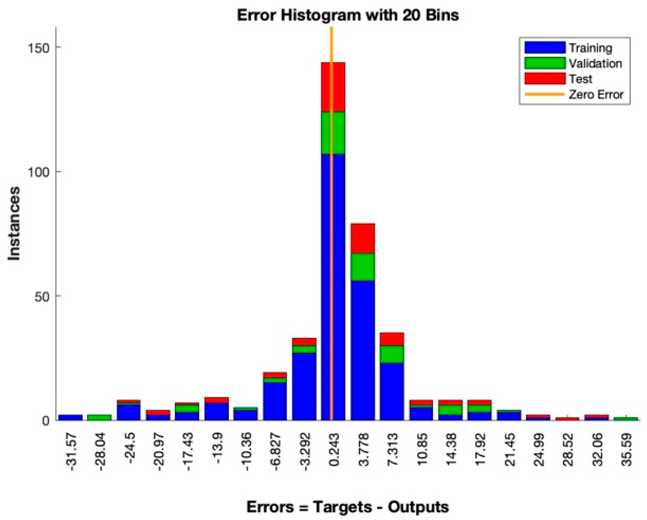
The first error that was calculated on 70% of the data, which refers exclusively to the training process, is highlighted in both applications based on LR = 0.1 by a histogram curve. As is visible, the error histogram curve calculated on the results obtained by the application of a Bayesian regularization training algorithm is not as low as the error calculated on the results obtained using the Levenberg–Marquardt algorithm (Figure 2). Using a Bayesian regularization algorithm, the error achieved during the training process was 20.9% on the length, 19.8% on the width, and 36.1 on the thickness, while using a Levenberg–Marquardt algorithm, it was, respectively, 20.3%, 19.8%, and 33.7%.

Instead, the error achieved in the final test using the Bayesian algorithm was 24.4% on the length, 18.8% on the width, and 42.4% on the thickness, while in the same test, using the Levenberg–Marquardt algorithm, it was, respectively, 36.4%, 25%, and 42.2% (Figure 7).

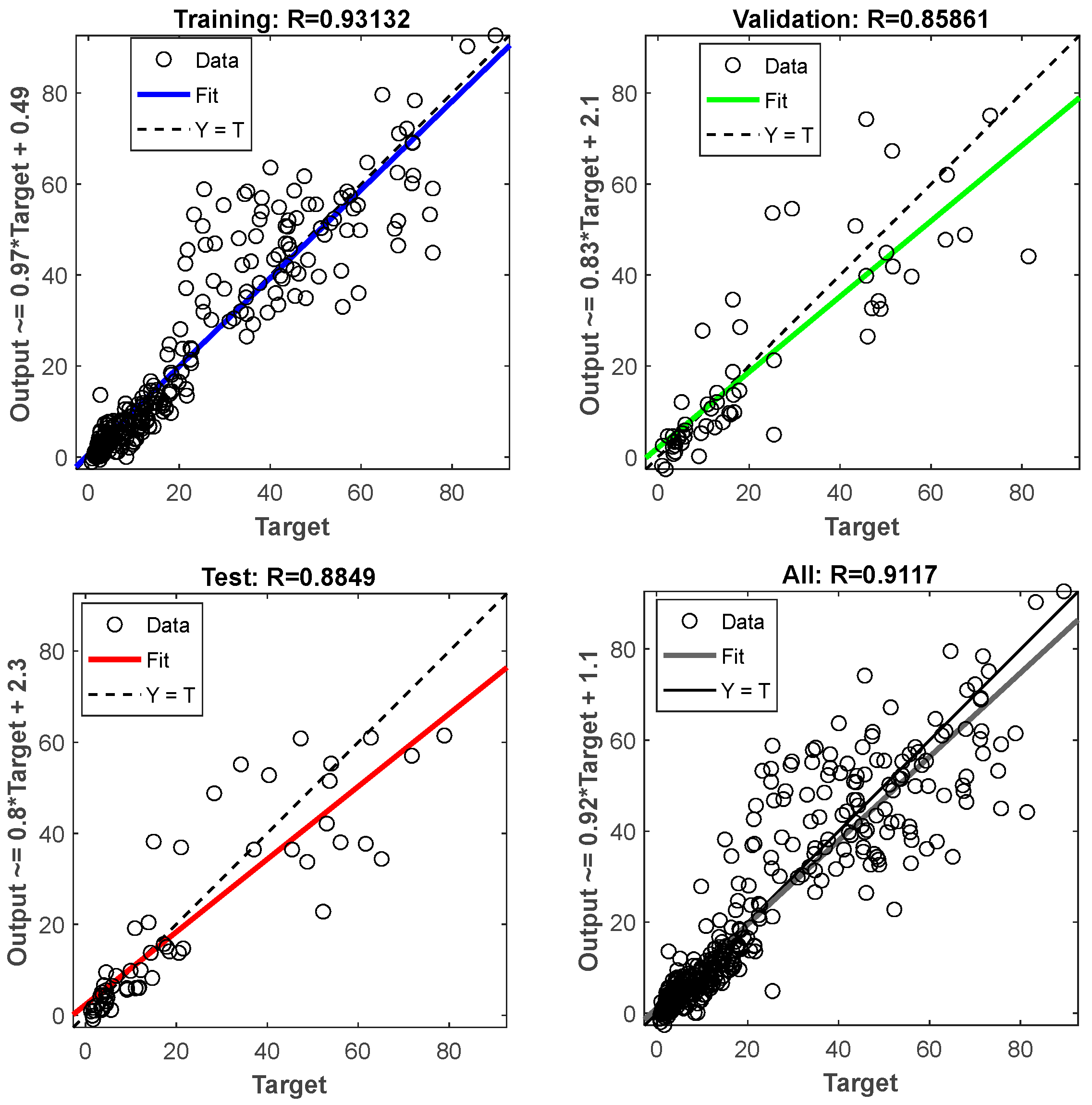
The regression line was obtained by using 70% of the data for training, validation, and testing. When applying the Bayesian regularization algorithm with LR = 0.1, it was found to have better control over overfitting issues during the training process compared to the Levenberg–Marquardt algorithm with the same rate (Figure 8). However, both algorithms resulted in a range of negative values.

The regression line made of the remaining 30% of the data (final test prediction) does not differ excessively from the previous test (data training prediction or “all”).

The application of a Bayesian algorithm produced results that were not affected by overfitting problems during the training prediction as they were instead using a Levenberg–Marquardt algorithm but, despite that, a range of negative values were obtained as well (Figure 9).

The negative values, even though they represent a small amount, are not compatible with the metrics prediction of real objects; they do not represent a theoretical model of metrics values that belong to “imaginary numbers” but to “real numbers”. Additionally, the errors obtained were not as minor as anticipated. Therefore, due to overfitting issues in the second application, we decided to move forward with a higher LR.

3.2. Bayesian vs. Levenberg–Marquardt Based on LR = 0.3

The LR = 0.3 test showed better efficacy, without any negative values or overfitting problems. The Bayesian regularization algorithm showed a better response than the Levenberg–Marquardt one. A lower error rate indeed characterized the first algorithm.

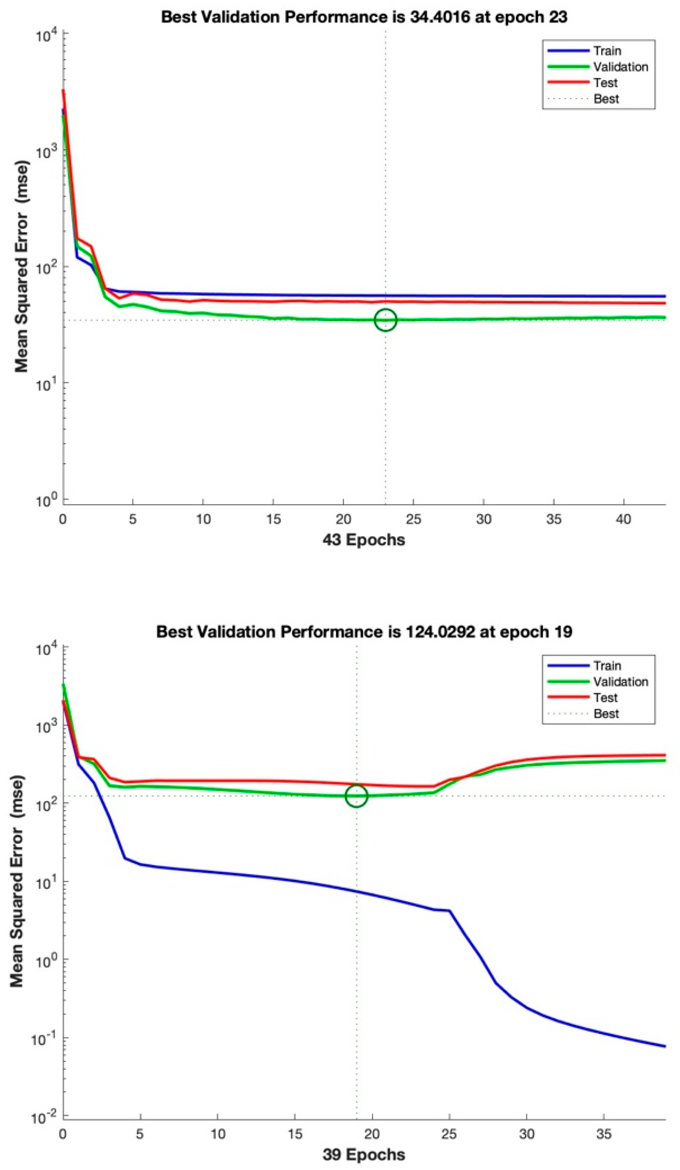
The application of a Bayesian regularization algorithm based on LR = 0.3 reached its best validation performance of 34.4016 at epoch 23, and stopped at epoch 43 with no better results. The use of a Levenberg–Marquardt algorithm instead reached its best validation performance of 124.0292 at epoch 19 and stopped at epoch 39 with no better outcome (Figure 10).

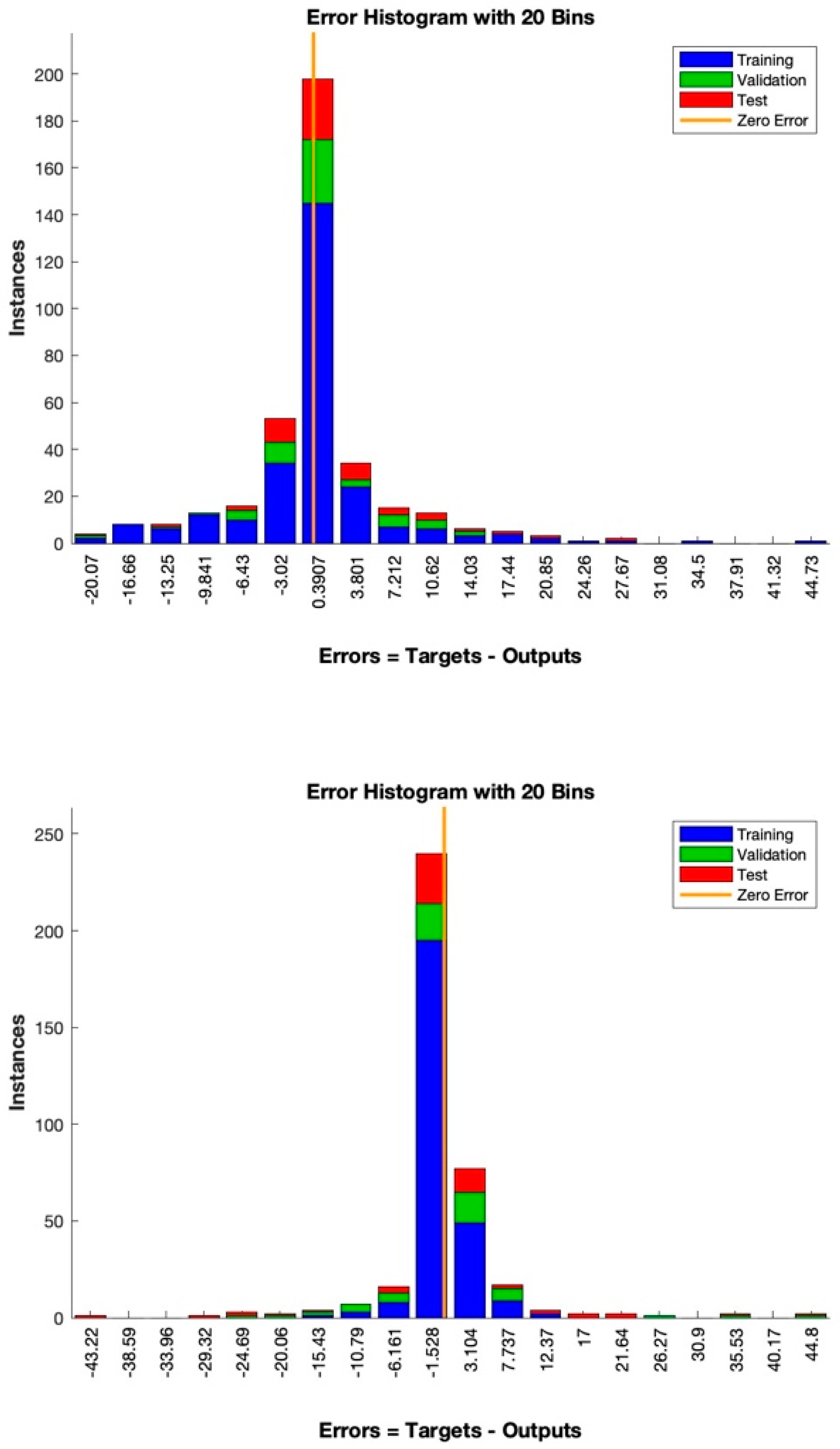
As with the previous test set on LR = 0.1, the error of the following one based on LR = 0.3 was calculated both automatically on 70% of the data and separately on a previously established 30% of the data. The error calculated on the first group showed in both cases a good response during the training, validation, and test processes, especially using the Bayesian regularization algorithm. The Levenberg–Marquardt algorithm suffered from overfitting problems during the training process. For this reason, the histogram showed a lower error than the Bayesian algorithm, while this represented a more realistic error curve during the training, which was not affected by overfitting problems (Figure 11).

The error calculated separately on the remaining 30% of the data differed substantially from each of the selected algorithms. The error obtained by applying the Bayesian algorithm showed incredibly low error rates during both the test and the training. The error on the total length prediction of damaged artifacts was 19.6% during the test and 23.9% during the training; the error achieved on the distal width prediction was, respectively, 12.5% and 19.7%; and the error acquired on the distal thickness prediction was, respectively, 25.1% and 34.4%.

The error achieved using the Levenberg–Marquardt algorithm instead showed higher error rates during the test but not during the training. The error rate on the total length prediction of fragmented artifacts was indeed 44.3% during the test and 15.2% during the training; the error obtained on the distal width prediction of these artifacts was, respectively, 26.1/% and 13%. Finally, the error achieved on artifacts’ distal thickness prediction was, respectively, 51% and 29.4%.

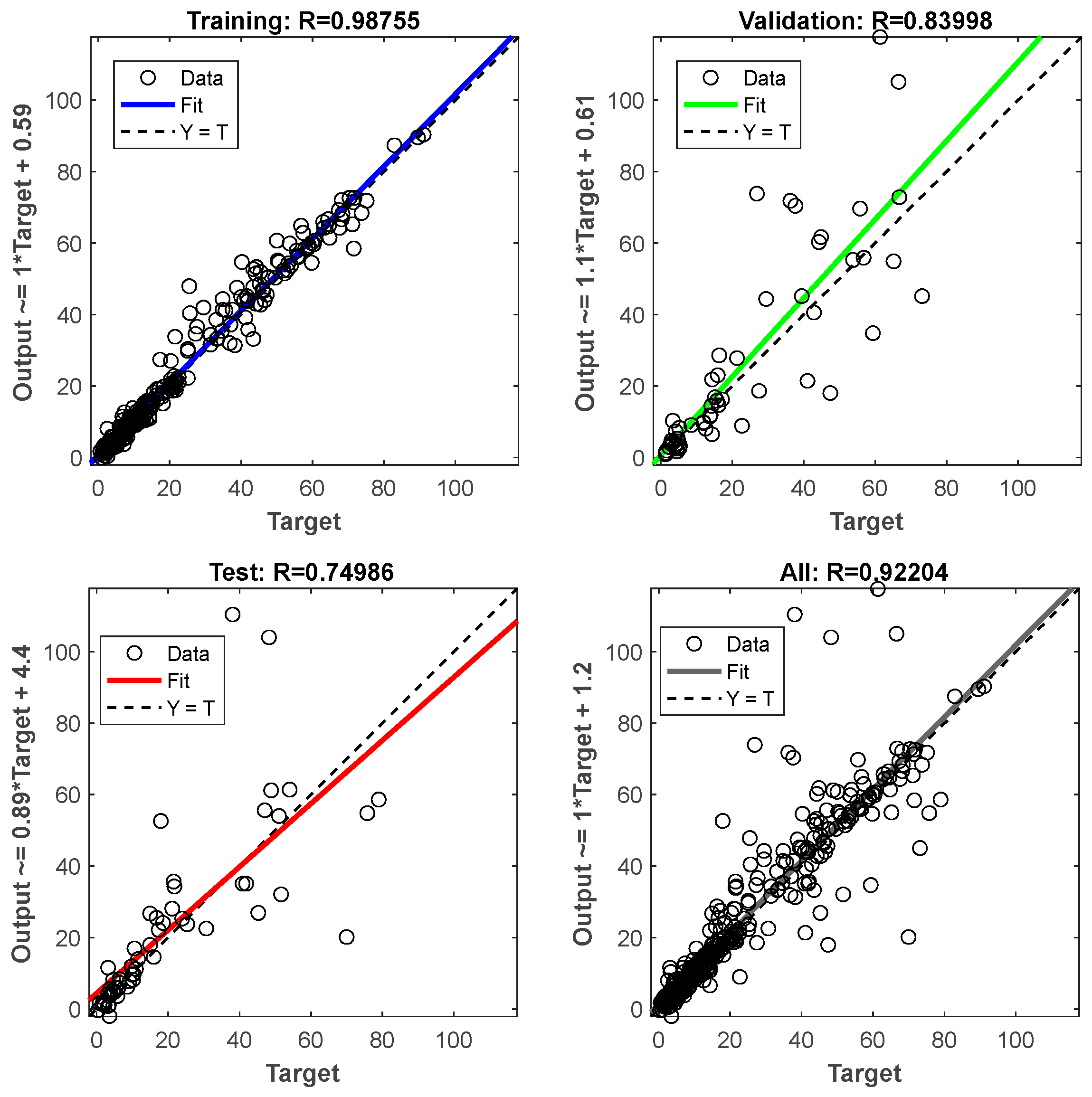
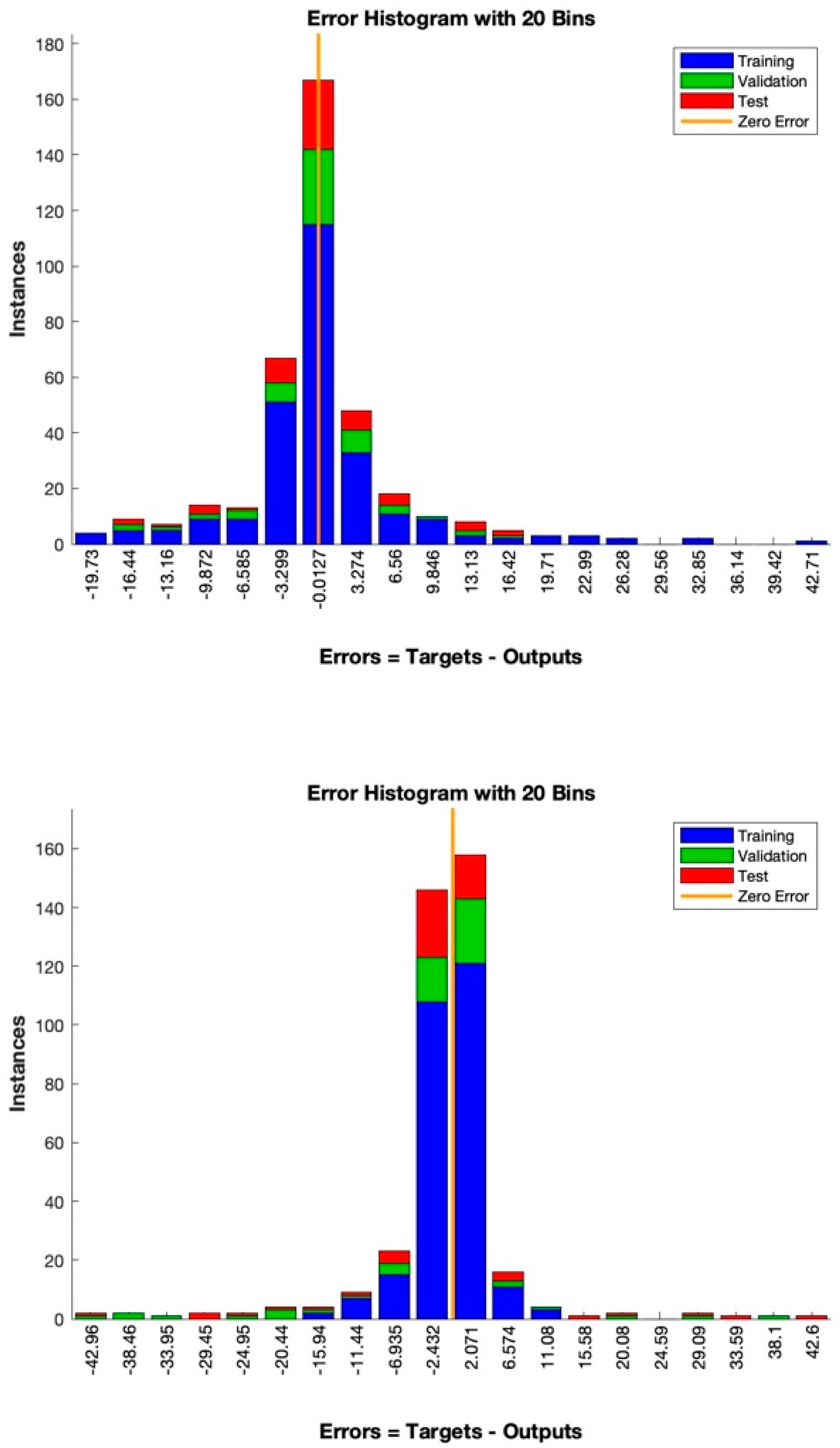
The regression lines of each application indeed showed how differently the two algorithms worked and their diverse efficiency. The Bayesian regularization algorithm set on LR = 0.3 was not affected by overfitting problems either during the training process carried out automatically on the first group of artifacts subdivided in 70% of the data or during the test carried out on the remaining 30% that belong to the same group. Instead, the Levenberg–Marquardt algorithm showed in both cases a high inefficacy due to overfitting problems that led to only an apparently lower error rate calculated on the first group of data composed of 70% of them (Figure 12). The error calculated on the second group indeed showed higher error rates due to the impossibility of this algorithm being able to process these data properly.

Concerning the regression lines carried out on the second group of artifacts composed of 30% of the data pulled out from the neural network automatic analysis, they showed encouraging results that confirmed the previous regression line carried out on the first group of artifacts.

During both the training process and the final test, the regression lines were carried out using a Bayesian algorithm. The regression lines did not produce any negative values, as expected, and did not suffer from overfitting problems. As a result, the achieved regression lines accurately represented a real range of dimensional metrics for the laminar artifacts.

During both the training and validation processes, a Levenberg–Marquardt algorithm was applied, but it was unsuccessful in preventing negative values and overfitting issues (Figure 13).

The application of LR = 0.3 showed positive results and a high level of efficacy using the Bayesian regularization algorithm; instead, the same rate based on the Levenberg–Marquardt algorithm did not provide the expected results.

To verify the possibility of achieving better results based on the application of the Bayesian regularization algorithm or to confirm the inefficiency of the Levenberg–Marquardt algorithm for this purpose, we decided to move forward to another step, increasing the learning rate for each application.

3.3. Bayesian vs. Levenberg–Marquardt Based on LR = 0.4

Both the Bayesian regularization and the Levenberg–Marquardt training algorithms based on LR = 0.4 showed positive but limited results, proving the boundaries of their application.

The best validation performance achieved with the application of a Bayesian regularization algorithm was 1916.6449 at epoch 9, and it stopped after 19 epochs without any amelioration. The best validation performance obtained with a Levenberg–Marquardt algorithm was instead 1105.7728 at epoch 8, and it stopped after 18 epochs without any better result (Figure 14).

Following the same procedure shown above, the errors were calculated on both the training set of data (70% of data) and the test set of data (30% of data). The error range calculated on the first group shown as well as the application of both the algorithms set on LR = 0.1 revealed the presence of negative values, and the existence of a misleading low error concerning the Levenberg–Marquardt algorithm, which represents overfitting problems (Figure 15).

The error calculated on the second group of data showed a high efficacy rate during both the training and test of the metrics prediction based on the Bayesian algorithm set on LR = 0.4. The predicted errors of the fragmented artifacts’ length, distal width, and distal thickness prediction were indeed, respectively, 20.8%, 17%, and 43.5% during the training, and 16.9%, 26.6%, and 34.8% during the test. Instead, the Levenberg–Marquardt algorithm set on LR = 0.4 achieved a higher error range. The metrics prediction errors obtained during the training process were, respectively, 20.9% on the length, 14.8% on the distal width, and 31.7% on the distal thickness, while the errors achieved during the final test were, respectively, 47.8% on the length, 48.7% on the distal width, and 74.3% on the distal thickness prediction.

The regression lines have indeed shown good results concerning the application of a Bayesian regularization algorithm based on LR = 0.4 during the training process and its internal validation and test. Neither negative values were produced during the metrics prediction nor overfitting problems affected the neural network. Finally, despite the use of a Levenberg–Marquardt algorithm set on LR = 0.4 not producing any negative predicted values, the overfitting problem affected the entire training process (Figure 16).

The regression lines carried out on the remaining 30% of the data that were not previously selected for the training process showed a similar tendency to the previous regression line analyzed on 70% of the data. The Bayesian regularization algorithm based on LR = 0.4 did not produce negative values, and the results were positive, even though they were not as positive as those achieved with LR = 0.3 during both the training and the final test. Instead, the regression curves obtained using a Levenberg–Marquardt algorithm were not only still affected by overfitting problems during the training process but also showed negative values during the validation prediction (Figure 17).

4. Conclusions

The analysis of a neural network application for predicting regular artifact metrics, such as Pre-Pottery Neolithic B laminar artifacts, showed positive results.

Our study compared the effectiveness of two algorithms, Levenberg–Marquardt and Bayesian regularization, in reconstructing dimensional lithic tools. While both algorithms performed well and did not show differences in terms of the computational cost (based on the same parameters), our experiments consistently showed that Bayesian regularization outperformed Levenberg–Marquardt across various performance metrics.

Specifically, the best results were achieved with the Bayesian regularization algorithm based on LR = 0.3, reaching an impressive reconstruction accuracy of 80.4% for the length prediction, 87.5% for the width prediction, and 74.9% for the thickness prediction. Instead, the best results were achieved with the Levenberg–Marquardt algorithm set on LR = 0.1. In particular, the level of accuracy was 63.6% for the length prediction, 75% for the width prediction, and 57.8% for the thickness prediction. Additionally, Bayesian regularization had a minor tendency to overfit, with a lower variance in the reconstruction errors than Levenberg–Marquardt.

Our study highlighted the importance of algorithm selection and parameter tuning in achieving optimal reconstruction results. While Levenberg–Marquardt is a viable option, Bayesian regularization is the preferred choice for more complex dimensional lithic tool reconstruction tasks.

For future research, we recommend exploring additional regularization techniques and advanced model architectures to enhance the reconstruction accuracy and scalability in real-world applications. It would also be interesting to test the performance of Bayesian regularization on small datasets.

Despite the challenge of limited data, we leveraged a complex neural network architecture to fix the underfitting issues. However, this approach raised concerns about overfitting. By implementing Bayesian regularization, we effectively regulated the model complexity and achieved remarkable reconstruction accuracy even with our constrained dataset.

It is worth noting that the level of precision in the engineering sciences is typically deemed ideal at around 80 to 90%. However, this particular case study centers on handmade goods that were crafted 10 millennia ago, well prior to the advent of industrialization. As such, the findings of this study hold tremendous significance from an archaeological standpoint, as they provide mathematical confirmation of the notion of standardizing chipping practices in order to achieve consistent laminar products.

The results of this study were indeed quite remarkable, revealing a high degree of technological uniformity in the size and shape of laminar blanks. Notably, the users of such blades might have tended to maintain a consistent width, which allowed for practical handling, a reason that might explain the higher accuracy of this metric compared to the others.

Furthermore, this study provided a fascinating insight into the cultural practices of the time, showcasing a shared cultural foundation that prioritized a meticulously controlled approach to laminar blank production. The study demonstrated a remarkable ability to anticipate the size of fragmented laminar blanks, underscoring the predictive power of the research and its potential for further discoveries. The accuracy of the predictions highlights the efficacy of the methodology employed and the depth of understanding of the underlying principles.

References

1. Guyot, A.; Lennon, M.; Lorho, T.; Hubert-Moy, L. Combined Detection and Segmentation of Archeological Structures from LiDAR Data Using a Deep Learning Approach. J. Comput. Appl. Archaeol. 2021, 4, 1. [Google Scholar] [CrossRef]
2. Scotland, A.; Øivind, T.; David, C.; Waldeland, U.A. Using deep neural networks on airborne laser scanning data: Results from a case study of semi-automatic mapping of archaeological topography. Archaeol. Prospect. 2018, 26, 165–175. [Google Scholar] [CrossRef]
3. Caspari, G.; Crespo, B. Convolutional neural networks for archaeological site detection—Finding “princely” tombs. J. Archaeol. Sci. 2019, 110, 104998. [Google Scholar] [CrossRef]
4. Davis, D.S.; Caspari, G.; Lipo, C.P.; Sanger, M.C. Deep Learning Reveals Extent of Archaic Native American Shell-Ring Building Practices. J. Archaeol. Sci. 2021, 132, 105433. [Google Scholar] [CrossRef]
5. Küçükdemirci, M.; Sarris, A. Deep learning based automated analysis of archaeo-geophysical images. Archaeol. Prospect. 2020, 27, 107–118. [Google Scholar] [CrossRef]
6. Trier, Ø.D.; Reksten, J.H.; Løseth, K. Automated mapping of cultural heritage in Norway from airborne lidar data using faster R-CNN. Int. J. Appl. Earth Obs. Geoinf. 2021, 95, 102241. [Google Scholar] [CrossRef]
7. Cole, K.E.; Yaworsky, P.M.; Hart, I.A. Evaluating statistical models for establishing morphometric taxonomic identifications and a new approach using Random Forest. J. Archaeol. Sci. 2022, 143, 105610. [Google Scholar] [CrossRef]
8. Eberl, M.; Bell, C.S.; Spencer-Smith, J.; Raj, M.; Sarubbi, A.; Johnson, P.S.; Rieth, A.E.; Chaudhry, U.; Aguila, R.E.; McBride, M. Machine Learning–Based Identification of Lithic Microdebitage. Adv. Archaeol. Pract. 2023, 11, 152–163. [Google Scholar] [CrossRef]
9. Gualandi, M.L.; Gattiglia, G.; Anichini, F. An Open System for Collection and Automatic Recognition of Pottery through Neural Network Algorithms. Heritage 2021, 4, 140–159. [Google Scholar] [CrossRef]
10. Saipraneeth, G.; Jyotindra, N.; Roger, A.S.; Sachin, S.G. A Bayesian regularization-backpropagation neural network model for peeling computations. J. Adhes. 2021, 99, 92–115. [Google Scholar] [CrossRef]
11. Barber, D. Bayesian Reasoning and Machine Learning; Cambridge University Press: Cambridge, UK, 2012. [Google Scholar]
12. Sapna, S.; Tamilarasi, A.; Pravin, M.K. Backpropagation Learning Algorithm Based on Levenberg Marquardt Algorithm. Comput. Sci. Inf. Technol. 2012, 2, 393–398. [Google Scholar] [CrossRef]
13. Qian, N. On the momentum term in gradient descent learning algorithms. Neural Netw. 1999, 12, 145–151. [Google Scholar] [CrossRef] [PubMed]
14. Arimura, M. The Neolithic Lithic Industry at Tell Ain El-Kerkh; Archaeopress Archaeology: Oxford, UK, 2020. [Google Scholar]
15. Shea, J.J. Stone Tools in the Palaeolithic and Neolithic Near East: A Guide; Cambridge University Press: New York, NY, USA, 2013. [Google Scholar]
16. Barzilai, O. Social Complexity in the Southern Levantine PPNB as Reflected through Lithic Studies: The Bidirectional Blade Industries; BAR International Series; Archaeopress: Oxford, UK, 2010. [Google Scholar]
17. Nobile, E.; Conati, C.B. The Standardisation of the PPNB Lithic Industry from Er-Rahib. Orig. Rev. Prehistory Protohistory Anc. Civiliz. 2022, 46, 7–28. [Google Scholar]
18. Sariev, E.; Germano, G. Bayesian regularized artificial neural networks for the estimation of the probability of default. Quant. Financ. 2020, 20, 311–328. [Google Scholar] [CrossRef]
19. Reynaldi, A.; Lukas, S.; Margaretha, H. Backpropagation and Levenberg-Marquardt Algorithm for Training Finite Element Neural Network. In Proceedings of the 2012 Sixth UKSim/AMSS European Symposium on Computer Modeling and Simulation, Valletta, Malta, 14–16 November 2012. [Google Scholar]
Figure 1. Technological measurements.
Information 15 00270 g001
Figure 2. Laminar artifacts from Nahal Reuel (ad), Yiftahel (e,f), and Motza (gj). Undamaged laminar artifacts (a,c,e,g,i) and laminar artifacts with missing distal ends (b,d,f,h,j).
Information 15 00270 g002
Figure 3. Example of a neural network with an architecture based on two hidden layers.
Information 15 00270 g003
Figure 4. Example of perceptron i in a hidden layer k R(s) activation function.
Information 15 00270 g004
Figure 5. Example of a sigmoid function.
Information 15 00270 g005
Figure 6. Best validation performance based on LR = 0.1. Bayesian regularization algorithm (top). Levenberg–Marquardt regularization algorithm (bottom). The regression curve was carried out on training data.
Information 15 00270 g006
Figure 7. Error histogram during training validation and test processes based on LR = 0.1. Bayesian regularization algorithm (top). Levenberg–Marquardt regularization algorithm (bottom).
Information 15 00270 g007aInformation 15 00270 g007b
Figure 8. Regression lines during training, validation, test, and merged processes based on LR = 0.1. Bayesian regularization algorithm (top). Levenberg–Marquardt regularization algorithm (bottom). The analysis was carried out on 70% of the total data.
Information 15 00270 g008aInformation 15 00270 g008b
Figure 9. Regression lines during training prediction (a) and final test (c), both using a Bayesian regularization training algorithm based on LR = 0.1. Regression line during training prediction (b) and final test (d), both using a Levenberg–Marquardt regularization training algorithm based on LR = 0.1.
Information 15 00270 g009
Figure 10. Best validation performance based on LR = 0.3. Bayesian regularization algorithm (top). Levenberg–Marquardt regularization algorithm (bottom). The regression curve was carried out on training data.
Information 15 00270 g010
Figure 11. Error histogram during training validation and test processes based on LR = 0.3. Bayesian regularization algorithm (top). Levenberg–Marquardt regularization algorithm (bottom).
Information 15 00270 g011
Figure 12. Regression lines during training, validation, test, and merged processes based on LR = 0.3. Bayesian regularization algorithm (top). Levenberg–Marquardt regularization algorithm (bottom). The analysis was carried out on 70% of the total data.
Information 15 00270 g012
Figure 13. Regression lines during training prediction (a) and final test (c), both using a Bayesian regularization training algorithm based on LR = 0.3. Regression lines during training prediction (b) and final test (d), both using a Levenberg–Marquardt regularization training algorithm based on LR = 0.3.
Information 15 00270 g013
Figure 14. Best validation performance based on LR = 0.4. Bayesian regularization algorithm (top). Levenberg–Marquardt regularization algorithm (bottom). The regression line was carried out on training data.
Information 15 00270 g014
Figure 15. Error histogram during training validation and test processes based on LR = 0.4. Bayesian regularization algorithm (top). Levenberg–Marquardt regularization algorithm (bottom).
Information 15 00270 g015
Figure 16. Regression lines during training, validation, test, and merged processes based on LR = 0.4. Bayesian regularization algorithm (top). Levenberg–Marquardt regularization algorithm (bottom). The analysis was carried out on 70% of the total data.
Information 15 00270 g016
Figure 17. Regression lines during training prediction (a) and final test (c), both using a Bayesian regularization training algorithm based on LR = 0.4. Regression lines during training prediction (b) and final test (d), both using a Levenberg–Marquardt regularization training algorithm based on LR = 0.4.
Information 15 00270 g017
Disclaimer/Publisher’s Note: The statements, opinions and data contained in all publications are solely those of the individual author(s) and contributor(s) and not of MDPI and/or the editor(s). MDPI and/or the editor(s) disclaim responsibility for any injury to people or property resulting from any ideas, methods, instructions or products referred to in the content.