
Improving the Classification of Unexposed Potsherd Cavities by Means of Preprocessing

 , , , ,
Abstract
1. Introduction
- It investigates the impact of image preprocessing methods on classification accuracy in detail.
- It thoroughly examines image preprocessing techniques on distinct datasets, including controlled laboratory-made images and real-world potsherd objects discovered in archaeological sites.
- It enhances performance compared to the previous study by identifying the most effective image preprocessing method.
2. Materials and Methods
2.1. Image Preprocessing
2.2. Smoothing and Sharpening
2.3. Rotations, Flips, and Transposition
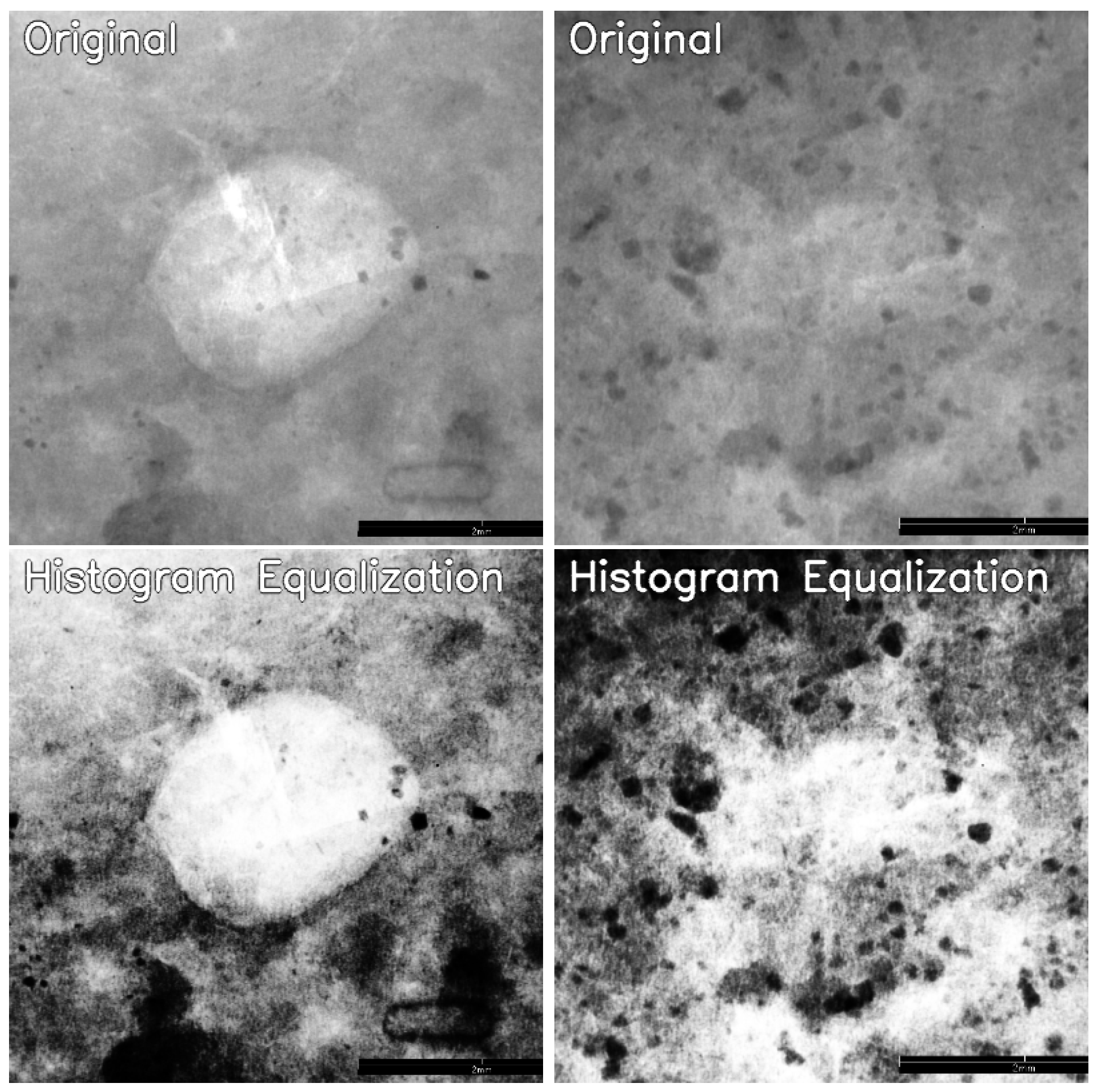
2.4. Histogram Equalization
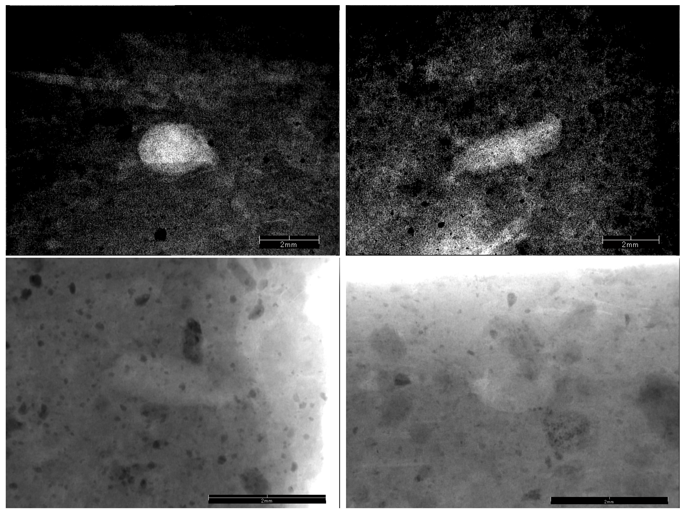
2.5. Adaptive Histogram Equalization
2.6. Grid Distortion and Elastic Transformation
3. Experimental Setup
3.1. Environment Setup
3.2. Classification Model
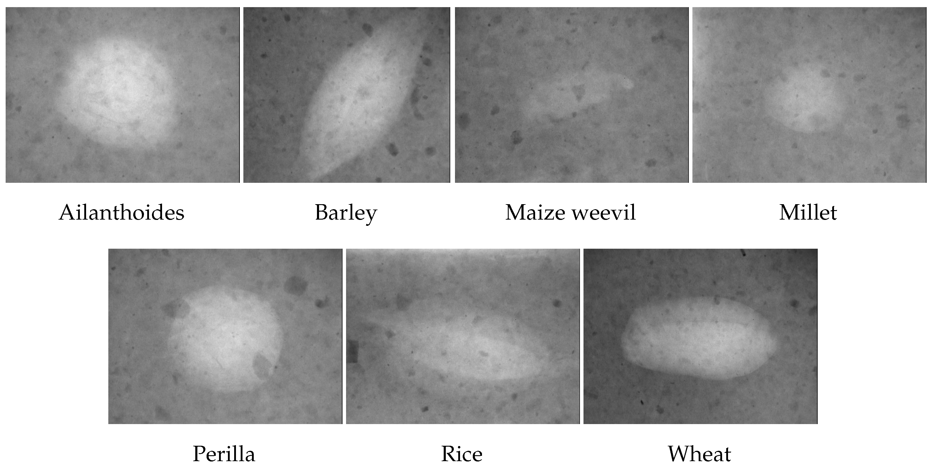
3.3. Dataset
3.4. Learning Rate
4. Results and Discussion
4.1. Single Methods
4.1.1. Histogram Equalization
4.1.2. Adaptive Histogram Equalization
4.1.3. Smoothing
4.1.4. Sharpening
4.1.5. Rotations, Flips, and Transposition
4.1.6. Grid Distortion and Elastic Transformation
4.2. Combination Methods
4.2.1. Adaptive Histogram Equalization and Smoothing
4.2.2. Rotations, Flips, and Transposition
4.2.3. Rotations, Flips, Transposition, Grid Distortion, and Elastic Transformation
4.2.4. Adaptive Histogram Equalization, Smoothing, Rotations, Flips, and Transposition
4.2.5. Adaptive Histogram Equalization, Rotations, Flips, and Transposition
4.3. K-Fold Cross-Validation
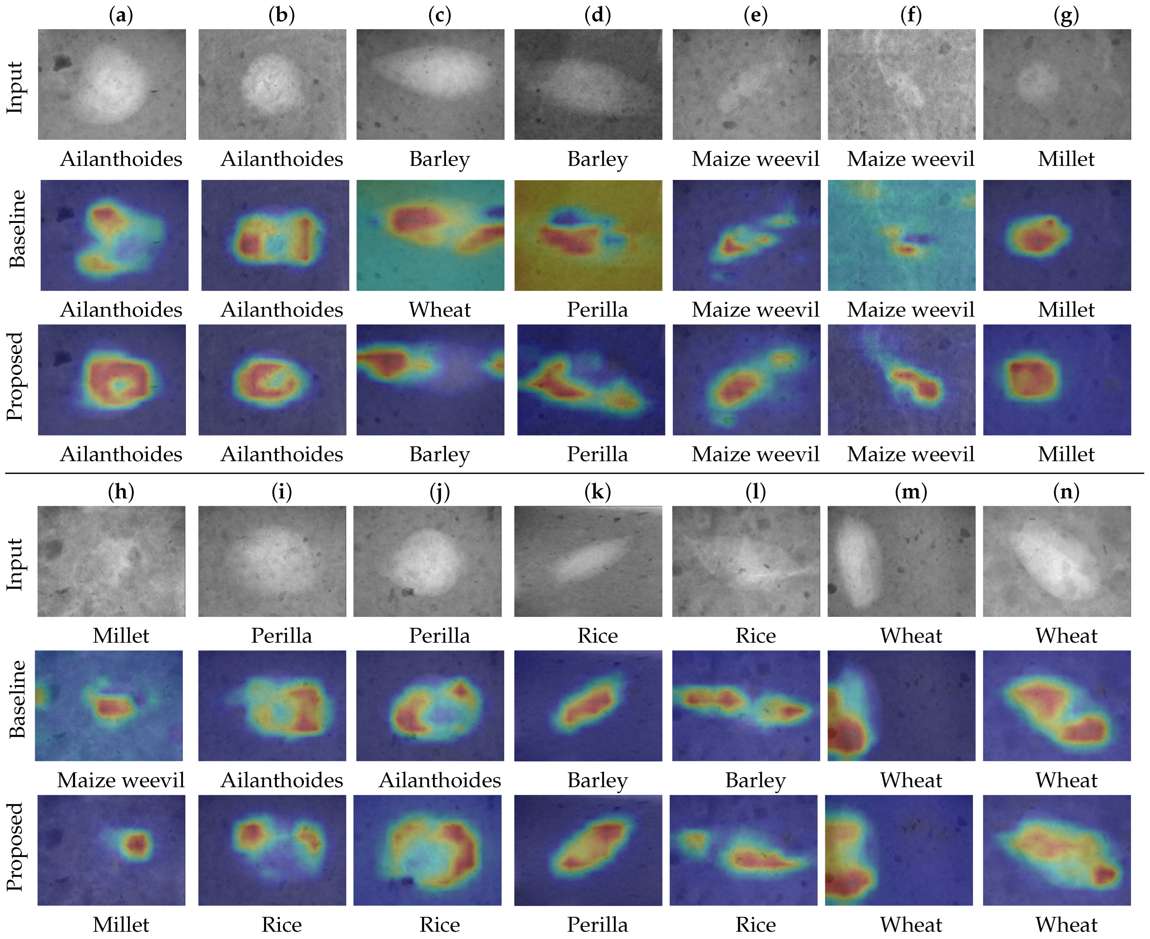
4.4. Class Activation Maps (CAMs)
5. Conclusions
Author Contributions
Funding
Institutional Review Board Statement
Informed Consent Statement
Data Availability Statement
Conflicts of Interest
References
- Sajedi, H.; Pardakhti, N. Age Prediction Based on Brain MRI Image: A Survey. J. Med. Syst. 2019, 43, 279. [Google Scholar] [CrossRef]
- Ullah, Z.; Farooq, M.U.; Lee, S.H.; An, D. A hybrid image enhancement based brain MRI images classification technique. Med. Hypotheses 2020, 143, 109922. [Google Scholar] [CrossRef]
- ul Rehman, A.; Qureshi, S.A. A review of the medical hyperspectral imaging systems and unmixing algorithms’ in biological tissues. Photodiagnosis Photodyn. Ther. 2021, 33, 102165. [Google Scholar] [CrossRef]
- Zhang, X.; Ma, Y.; Gong, Q.; Yao, J. Automatic detection of microaneurysms in fundus images based on multiple preprocessing fusion to extract features. Biomed. Signal Process. Control 2023, 85, 104879. [Google Scholar] [CrossRef]
- Ahamed, K.U.; Islam, M.; Uddin, A.; Akhter, A.; Paul, B.K.; Yousuf, M.A.; Uddin, S.; Quinn, J.M.; Moni, M.A. A deep learning approach using effective preprocessing techniques to detect COVID-19 from chest CT-scan and X-ray images. Comput. Biol. Med. 2021, 139, 105014. [Google Scholar] [CrossRef]
- Sarwinda, D.; Paradisa, R.H.; Bustamam, A.; Anggia, P. Deep Learning in Image Classification using Residual Network (ResNet) Variants for Detection of Colorectal Cancer. Procedia Comput. Sci. 2021, 179, 423–431. [Google Scholar] [CrossRef]
- Shakeel, P.M.; Burhanuddin, M.; Desa, M.I. Lung cancer detection from CT image using improved profuse clustering and deep learning instantaneously trained neural networks. Measurement 2019, 145, 702–712. [Google Scholar] [CrossRef]
- Mall, P.K.; Singh, P.K.; Yadav, D. GLCM Based Feature Extraction and Medical X-RAY Image Classification using Machine Learning Techniques. In Proceedings of the 2019 IEEE Conference on Information and Communication Technology, Allahabad, India, 6–8 December 2019; pp. 1–6. [Google Scholar]
- Heidari, M.; Mirniaharikandehei, S.; Khuzani, A.Z.; Danala, G.; Qiu, Y.; Zheng, B. Improving the performance of CNN to predict the likelihood of COVID-19 using chest X-ray images with preprocessing algorithms. Int. J. Med. Inform. 2020, 144, 104284. [Google Scholar] [CrossRef]
- Mungra, D.; Agrawal, A.; Sharma, P.; Tanwar, S.; Obaidat, M.S. Pratit: A CNN-based emotion recognition system using histogram equalization and data augmentation. Multimed. Tools Appl. 2019, 79, 2285–2307. [Google Scholar] [CrossRef]
- Beeravolu, A.R.; Azam, S.; Jonkman, M.; Shanmugam, B.; Kannoorpatti, K.; Anwar, A. Preprocessing of Breast Cancer Images to Create Datasets for Deep-CNN. IEEE Access 2021, 9, 33438–33463. [Google Scholar] [CrossRef]
- Sarki, R.; Ahmed, K.; Wang, H.; Zhang, Y.; Ma, J.; Wang, K. Image preprocessing in classification and identification of diabetic eye diseases. Data Sci. Eng. 2021, 6, 455–471. [Google Scholar] [CrossRef] [PubMed]
- Mendonça, I.; Miyaura, M.; Fatyanosa, T.N.; Yamaguchi, D.; Sakai, H.; Obata, H.; Aritsugi, M. Classification of unexposed potsherd cavities by using deep learning. J. Archaeol. Sci. Rep. 2023, 49, 104003. [Google Scholar] [CrossRef]
- Masoudi, S.; Harmon, S.A.A.; Mehralivand, S.; Walker, S.M.; Raviprakash, H.; Bagci, U.; Choyke, P.L.; Turkbey, B. Quick guide on radiology image pre-processing for deep learning applications in prostate cancer research. J. Med. Imaging 2021, 8, 010901. [Google Scholar] [CrossRef] [PubMed]
- Gonzalez, R.C.; Woods, R.E. Digital Image Processing, 4th ed.; Prentice Hall: Hoboken, NJ, USA, 2007. [Google Scholar]
- Wang, S.; Celebi, M.E.; Zhang, Y.D.; Yu, X.; Lu, S.; Yao, X.; Zhou, Q.; Miguel, M.G.; Tian, Y.; Gorriz, J.M.; et al. Advances in Data Preprocessing for Biomedical Data Fusion: An Overview of the Methods, Challenges, and Prospects. Inf. Fusion 2021, 76, 376–421. [Google Scholar] [CrossRef]
- Kaur, C.; Garg, U. Artificial intelligence techniques for cancer detection in medical image processing: A review. Mater. Today Proc. 2023, 81, 806–809. [Google Scholar] [CrossRef]
- Chlap, P.; Min, H.; Vandenberg, N.; Dowling, J.; Holloway, L.; Haworth, A. A review of medical image data augmentation techniques for deep learning applications. J. Med. Imaging Radiat. Oncol. 2021, 65, 545–563. [Google Scholar] [CrossRef] [PubMed]
- Khalifa, N.E.; Loey, M.; Mirjalili, S. A comprehensive survey of recent trends in deep learning for digital images augmentation. Artif. Intell. Rev. 2022, 55, 2351–2377. [Google Scholar] [CrossRef] [PubMed]
- Zheng, Q.; Yang, M.; Tian, X.; Jiang, N.; Wang, D. A Full Stage Data Augmentation Method in Deep Convolutional Neural Network for Natural Image Classification. Discret. Dyn. Nat. Soc. 2020, 2020, 4706576. [Google Scholar] [CrossRef]
- Elgendi, M.; Nasir, M.U.; Tang, Q.; Smith, D.; Grenier, J.P.; Batte, C.; Spieler, B.; Leslie, W.D.; Menon, C.; Fletcher, R.R.; et al. The Effectiveness of Image Augmentation in Deep Learning Networks for Detecting COVID-19: A Geometric Transformation Perspective. Front. Med. 2021, 8, 629134. [Google Scholar] [CrossRef]
- Dhal, K.G.; Das, A.; Ray, S.; Gálvez, J.; Das, S. Histogram equalization variants as optimization problems: A Review. Arch. Comput. Methods Eng. 2020, 28, 1471–1496. [Google Scholar] [CrossRef]
- Alwazzan, M.J.; Ismael, M.A.; Ahmed, A.N. A hybrid algorithm to enhance colour retinal fundus images using a wiener filter and clahe. J. Digit. Imaging 2021, 34, 750–759. [Google Scholar] [CrossRef] [PubMed]
- Pizer, S.M.; Amburn, E.P.; Austin, J.D.; Cromartie, R.; Geselowitz, A.; Greer, T.; ter Haar Romeny, B.; Zimmerman, J.B.; Zuiderveld, K. Adaptive histogram equalization and its variations. Comput. Vision Graph. Image Process. 1987, 39, 355–368. [Google Scholar] [CrossRef]
- Sheet, S.S.M.; Tan, T.S.; As’ari, M.; Hitam, W.H.W.; Sia, J.S. Retinal disease identification using upgraded CLAHE filter and transfer convolution neural network. ICT Express 2022, 8, 142–150. [Google Scholar] [CrossRef]
- Opoku, M.; Weyori, B.A.; Adekoya, A.F.; Adu, K. Clahe-CapsNet: Efficient retina optical coherence tomography classification using capsule networks with contrast limited adaptive histogram equalization. PLoS ONE 2023, 18, e0288663. [Google Scholar] [CrossRef] [PubMed]
- Kuran, U.; Kuran, E.C. Parameter selection for Clahe using multi-objective cuckoo search algorithm for image contrast enhancement. Intell. Syst. Appl. 2021, 12, 200051. [Google Scholar] [CrossRef]
- Hussein, F.; Mughaid, A.; AlZu’bi, S.; El-Salhi, S.M.; Abuhaija, B.; Abualigah, L.; Gandomi, A.H. Hybrid CLAHE-CNN Deep Neural Networks for Classifying Lung Diseases from X-ray Acquisitions. Electronics 2022, 11, 3075. [Google Scholar] [CrossRef]
- Simard, P.; Steinkraus, D.; Platt, J. Best practices for convolutional neural networks applied to visual document analysis. In Proceedings of the Seventh International Conference on Document Analysis and Recognition, 2003, Proceedings, Edinburgh, Scotland, 3–6 August; 2003; pp. 958–963. [Google Scholar]
- Buslaev, A.; Iglovikov, V.I.; Khvedchenya, E.; Parinov, A.; Druzhinin, M.; Kalinin, A.A. Albumentations: Fast and Flexible Image Augmentations. Information 2020, 11, 125. [Google Scholar] [CrossRef]
- Liu, Z.; Mao, H.; Wu, C.Y.; Feichtenhofer, C.; Darrell, T.; Xie, S. A ConvNet for the 2020s. In Proceedings of the 2022 IEEE/CVF Conference on Computer Vision and Pattern Recognition (CVPR), New Orleans, LA, USA, 18–24 June 2022; pp. 11966–11976. [Google Scholar]
- He, K.; Zhang, X.; Ren, S.; Sun, J. Deep Residual Learning for Image Recognition. In Proceedings of the 2016 IEEE Conference on Computer Vision and Pattern Recognition (CVPR), Las Vegas, NV, USA, 27–30 June 2016; pp. 770–778. [Google Scholar]
- Kolesnikov, A.; Dosovitskiy, A.; Weissenborn, D.; Heigold, G.; Uszkoreit, J.; Beyer, L.; Minderer, M.; Dehghani, M.; Houlsby, N.; Gelly, S.; et al. An Image is Worth 16x16 Words: Transformers for Image Recognition at Scale. In Proceedings of the 9th International Conference on Learning Representations, Virtual, 3–7 May 2021. [Google Scholar]
- Liu, Z.; Lin, Y.; Cao, Y.; Hu, H.; Wei, Y.; Zhang, Z.; Lin, S.; Guo, B. Swin Transformer: Hierarchical Vision Transformer Using Shifted Windows. In Proceedings of the IEEE/CVF International Conference on Computer Vision (ICCV), 10, Virtual, 19–25 June 2021; pp. 10012–10022. [Google Scholar]
- Alwakid, G.; Gouda, W.; Humayun, M. Deep Learning-Based Prediction of Diabetic Retinopathy Using CLAHE and ESRGAN for Enhancement. Healthcare 2023, 11, 863. [Google Scholar] [CrossRef]
- Chen, S.; Li, Y.; Zhang, Y.; Yang, Y.; Zhang, X. Soft X-ray image recognition and classification of maize seed cracks based on image enhancement and optimized YOLOv8 model. Comput. Electron. Agric. 2024, 216, 108475. [Google Scholar] [CrossRef]
- Xiao, S.; Shen, X.; Zhang, Z.; Wen, J.; Xi, M.; Yang, J. Underwater image classification based on image enhancement and information quality evaluation. Displays 2024, 82, 102635. [Google Scholar] [CrossRef]
- Zhou, B.; Khosla, A.; Lapedriza, A.; Oliva, A.; Torralba, A. Learning Deep Features for Discriminative Localization. In Proceedings of the 2016 IEEE Conference on Computer Vision and Pattern Recognition (CVPR), Las Vegas, NV, USA, 26 June–1 July 2016; pp. 2921–2929. [Google Scholar]

| No. | Class | Number of Images | ||
|---|---|---|---|---|
| Train | Test | Jōmon–Yayoi | ||
| 1 | Ailanthoides | 134 | 15 | 8 |
| 2 | Barley | 127 | 15 | 0 |
| 3 | Maize weevil | 133 | 15 | 36 |
| 4 | Millet | 134 | 15 | 15 |
| 5 | Perilla | 135 | 15 | 3 |
| 6 | Rice | 132 | 15 | 2 |
| 7 | Wheat | 134 | 15 | 0 |
| Learning Rate | Accuracy (%) | |||
|---|---|---|---|---|
| Test Split | Jōmon–Yayoi Split | |||
| Max. | Avg. | Max. | Avg. | |
| 83.81 | 81.43 | 67.19 | 59.18 | |
| 82.86 | 79.29 | 68.75 | 63.87 | |
| 78.10 | 72.86 | 65.63 | 54.88 | |
| 79.05 | 67.98 | 53.13 | 42.97 | |
| Method | Accuracy (%) | Average Processing Times | ||||
|---|---|---|---|---|---|---|
| Test Split | Jōmon–Yayoi Split | Training | Inference | |||
| Avg. | Max. | Avg. | Max. | |||
| No preproc. | 80.48 | 84.76 | 60.16 | 62.50 | 0:35:15 | 0:00:02.1 |
| Histogram eq. | 75.24 | 80.00 | 60.35 | 65.63 | 0:22:45 | 0:00:02.5 |
| CLAHE-2 | 78.57 | 80.95 | 59.38 | 67.19 | 0:29:52 | 0:00:02.5 |
| CLAHE-3 | 79.88 | 82.86 | 64.45 | 70.31 | 0:33:00 | 0:00:02.5 |
| CLAHE-4 | 77.74 | 85.71 | 65.43 | 68.75 | 0:34:22 | 0:00:02.5 |
| CLAHE-5 | 79.64 | 83.81 | 65.43 | 70.31 | 0:35:45 | 0:00:02.5 |
| CLAHE-6 | 81.31 | 85.71 | 64.65 | 68.75 | 0:30:30 | 0:00:02.5 |
| CLAHE-7 | 79.05 | 81.90 | 63.09 | 68.75 | 0:35:37 | 0:00:02.4 |
| CLAHE-8 | 81.90 | 83.81 | 62.70 | 65.63 | 0:29:22 | 0:00:02.5 |
| Smooth-3 | 75.71 | 78.10 | 62.70 | 67.19 | 0:27:15 | 0:00:02.2 |
| Smooth-5 | 78.10 | 80.00 | 64.84 | 71.88 | 0:27:45 | 0:00:02.2 |
| Smooth-7 | 78.93 | 81.90 | 67.58 | 71.88 | 0:30:45 | 0:00:02.2 |
| Smooth-9 | 77.38 | 81.90 | 67.58 | 71.88 | 0:30:15 | 0:00:02.1 |
| Smooth-11 | 77.98 | 80.00 | 66.80 | 70.31 | 0:31:23 | 0:00:02.1 |
| Sharpen-0.2 | 79.40 | 81.90 | 60.55 | 68.75 | 0:26:00 | 0:00:02.1 |
| Sharpen-0.3 | 80.24 | 84.76 | 61.33 | 65.63 | 0:31:15 | 0:00:02.2 |
| Sharpen-0.4 | 80.48 | 82.86 | 59.57 | 67.19 | 0:32:00 | 0:00:02.1 |
| Sharpen-0.5 | 78.93 | 83.81 | 51.17 | 62.50 | 0:25:52 | 0:00:02.1 |
| V. flip (p) | 79.64 | 82.86 | 62.11 | 65.63 | 0:29:22 | 0:00:02.1 |
| V. flip+ | 80.24 | 82.86 | 62.70 | 70.31 | 0:56:45 | 0:00:02.1 |
| H. flip (p) | 83.10 | 85.71 | 59.77 | 67.19 | 0:29:00 | 0:00:02.1 |
| H. flip+ | 78.57 | 80.95 | 62.50 | 70.31 | 0:56:45 | 0:00:02.2 |
| All flips (p) | 81.90 | 84.76 | 62.50 | 67.19 | 0:32:15 | 0:00:02.1 |
| All flips+ | 81.79 | 86.67 | 65.43 | 67.19 | 1:40:52 | 0:00:02.1 |
| Transpose (p) | 81.67 | 83.81 | 63.67 | 68.75 | 0:32:00 | 0:00:02.1 |
| Transpose+ | 80.71 | 82.86 | 64.45 | 65.63 | 0:58:22 | 0:00:02.1 |
| Rotation 90+ | 79.88 | 81.90 | 65.04 | 68.75 | 1:00:15 | 0:00:02.1 |
| Rotation 180+ | 81.67 | 85.71 | 64.06 | 67.19 | 0:58:15 | 0:00:02.1 |
| Rotation 270+ | 81.67 | 85.71 | 65.04 | 70.31 | 0:54:00 | 0:00:02.1 |
| All Rotations (p) | 85.48 | 87.62 | 66.60 | 70.31 | 0:35:30 | 0:00:02.1 |
| All Rotations+ | 83.93 | 87.62 | 66.80 | 73.44 | 2:16:22 | 0:00:02.1 |
| Grid Distort. (p) | 82.02 | 84.76 | 66.80 | 68.75 | 0:30:22 | 0:00:02.1 |
| Grid Distort.+ | 79.88 | 81.90 | 65.63 | 73.44 | 0:52:22 | 0:00:02.1 |
| Elastic (p) | 80.12 | 81.90 | 63.28 | 68.75 | 0:39:00 | 0:00:02.1 |
| Elastic+ | 81.79 | 87.62 | 62.89 | 67.19 | 1:14:37 | 0:00:02.1 |
| Method | Accuracy (%) | Average Processing Times | ||||
|---|---|---|---|---|---|---|
| Test Split | Jōmon–Yayoi Split | Training | Inference | |||
| Avg. | Max. | Avg. | Max. | |||
| No preprocessing | 80.48 | 84.76 | 60.16 | 62.50 | 0:35:15 | 0:00:02.1 |
| Histogram. eq, smooth-9 | 70.00 | 74.29 | 61.33 | 64.06 | 0:25:22 | 0:00:02.7 |
| CLAHE-2, smooth-9 | 76.67 | 79.05 | 67.58 | 73.44 | 0:32:30 | 0:00:02.5 |
| CLAHE-3, smooth-9 | 77.02 | 80.95 | 66.99 | 70.31 | 0:29:37 | 0:00:02.4 |
| CLAHE-4, smooth-9 | 78.69 | 81.90 | 66.02 | 73.44 | 0:28:07 | 0:00:02.5 |
| CLAHE-5, smooth-9 | 79.17 | 80.95 | 69.92 | 75.00 | 0:31:00 | 0:00:02.5 |
| Rotate+, flips+ | 85.36 | 88.57 | 66.99 | 70.31 | 2:59:07 | 0:00:02.1 |
| Rotate+, transpose+ | 85.24 | 89.52 | 66.02 | 71.88 | 3:04:52 | 0:00:02.1 |
| Flips+, transpose+ | 82.50 | 89.52 | 65.82 | 70.31 | 1:47:22 | 0:00:02.1 |
| Rotate+, flip, transpose+ | 85.60 | 88.57 | 65.43 | 70.31 | 3:03:07 | 0:00:02.2 |
| Rotate+, flip+, transpose+ | 84.40 | 88.57 | 69.73 | 73.44 | 3:29:37 | 0:00:02.1 |
| Rotate+, flip+, transpose+, elastic | 83.69 | 86.67 | 68.16 | 71.88 | 4:30:15 | 0:00:02.1 |
| Rotate+, flip+, transpose+, elastic+ | 83.33 | 87.62 | 69.73 | 71.88 | 3:47:30 | 0:00:02.2 |
| Rotate+, flip+, transpose+, grid | 84.52 | 88.57 | 68.75 | 71.88 | 3:38:30 | 0:00:02.1 |
| Rotate+, flip+, transpose+, grid+ | 83.57 | 87.62 | 68.95 | 71.88 | 3:51:52 | 0:00:02.0 |
| CLAHE-2, smooth-9, rotate+, flip+, transpose+ | 82.50 | 85.71 | 68.95 | 73.44 | 3:07:45 | 0:00:02.4 |
| CLAHE-3, smooth-9, rotate+, flip+, transpose+ | 83.69 | 85.71 | 71.88 | 78.13 | 3:23:52 | 0:00:02.5 |
| CLAHE-4, smooth-9, rotate+, flip+, transpose+ | 84.05 | 88.57 | 66.80 | 71.88 | 3:55:30 | 0:00:02.4 |
| CLAHE-5, smooth-9, rotate+, flip+, transpose+ | 83.57 | 85.71 | 70.12 | 71.88 | 3:01:52 | 0:00:02.6 |
| CLAHE-6, smooth-9, rotate+, flip+, transpose+ | 83.45 | 85.71 | 71.29 | 78.13 | 3:07:00 | 0:00:02.5 |
| CLAHE-7, smooth-9, rotate+, flip+, transpose+ | 84.05 | 87.62 | 70.70 | 75.00 | 3:29:45 | 0:00:02.4 |
| CLAHE-8, smooth-9, rotate+, flip+, transpose+ | 82.02 | 84.76 | 72.46 | 76.56 | 3:01:15 | 0:00:02.4 |
| CLAHE-2, rotate+, flip+, transpose+ | 84.17 | 90.48 | 65.43 | 73.44 | 3:08:07 | 0:00:02.7 |
| CLAHE-3, rotate+, flip+, transpose+ | 84.40 | 85.71 | 64.84 | 73.44 | 3:44:30 | 0:00:02.4 |
| CLAHE-4, rotate+, flip+, transpose+ | 84.05 | 88.57 | 66.80 | 71.88 | 3:31:52 | 0:00:02.5 |
| CLAHE-5, rotate+, flip+, transpose+ | 82.38 | 85.71 | 63.28 | 71.88 | 2:57:52 | 0:00:02.5 |
| CLAHE-6, rotate+, flip+, transpose+ | 83.69 | 86.67 | 64.06 | 71.88 | 3:02:30 | 0:00:02.5 |
| CLAHE-7, rotate+, flip+, transpose+ | 84.88 | 86.67 | 69.14 | 73.44 | 3:40:00 | 0:00:02.6 |
| Fold | Accuracy (%) | |
|---|---|---|
| Test Split | Jōmon–Yayoi Split | |
| 1 | 88.57 | 68.75 |
| 2 | 87.62 | 71.88 |
| 3 | 82.86 | 70.31 |
| 4 | 80.95 | 76.56 |
| 5 | 87.62 | 64.06 |
| 6 | 84.76 | 70.31 |
| 7 | 80.95 | 73.44 |
| 8 | 82.86 | 76.56 |
| 9 | 85.71 | 71.88 |
| 10 | 92.38 | 73.44 |
| Average | 85.43 | 71.72 |
Disclaimer/Publisher’s Note: The statements, opinions and data contained in all publications are solely those of the individual author(s) and contributor(s) and not of MDPI and/or the editor(s). MDPI and/or the editor(s) disclaim responsibility for any injury to people or property resulting from any ideas, methods, instructions or products referred to in the content. |
© 2024 by the authors. Licensee MDPI, Basel, Switzerland. This article is an open access article distributed under the terms and conditions of the Creative Commons Attribution (CC BY) license (https://creativecommons.org/licenses/by/4.0/).
Share and Cite
Wihandika, R.C.; Lee, Y.; Data, M.; Aritsugi, M.; Obata, H.; Mendonça, I. Improving the Classification of Unexposed Potsherd Cavities by Means of Preprocessing. Information 2024, 15, 243. https://doi.org/10.3390/info15050243
Wihandika RC, Lee Y, Data M, Aritsugi M, Obata H, Mendonça I. Improving the Classification of Unexposed Potsherd Cavities by Means of Preprocessing. Information. 2024; 15(5):243. https://doi.org/10.3390/info15050243
Chicago/Turabian StyleWihandika, Randy Cahya, Yoonji Lee, Mahendra Data, Masayoshi Aritsugi, Hiroki Obata, and Israel Mendonça. 2024. "Improving the Classification of Unexposed Potsherd Cavities by Means of Preprocessing" Information 15, no. 5: 243. https://doi.org/10.3390/info15050243
APA StyleWihandika, R. C., Lee, Y., Data, M., Aritsugi, M., Obata, H., & Mendonça, I. (2024). Improving the Classification of Unexposed Potsherd Cavities by Means of Preprocessing. Information, 15(5), 243. https://doi.org/10.3390/info15050243