Article

Quantum Convolutional Long Short-Term Memory Based on Variational Quantum Algorithms in the Era of NISQ

1
School of Software, Nanjing University of Information Science and Technology, Nanjing 210044, China
2
School of Computer Science, Nanjing University of Information Science and Technology, Nanjing 210044, China
3
Wuxi Institute of Technology, Nanjing University of Information Science & Technology, Wuxi 214000, China
4
Jiangsu Collaborative Innovation Center of Atmospheric Environment and Equipment Technology (CICAEET), Nanjing University of Information Science and Technology, Nanjing 210044, China
*
Author to whom correspondence should be addressed.
Information 2024, 15(4), 175; https://doi.org/10.3390/info15040175
Submission received: 19 February 2024 / Revised: 16 March 2024 / Accepted: 20 March 2024 / Published: 22 March 2024
(This article belongs to the Special Issue Quantum Information Processing and Machine Learning)

Abstract

:
In the era of noisy intermediate-scale quantum (NISQ) computing, the synergistic collaboration between quantum and classical computing models has emerged as a promising solution for tackling complex computational challenges. Long short-term memory (LSTM), as a popular network for modeling sequential data, has been widely acknowledged for its effectiveness. However, with the increasing demand for data and spatial feature extraction, the training cost of LSTM exhibits exponential growth. In this study, we propose the quantum convolutional long short-term memory (QConvLSTM) model. By ingeniously integrating classical convolutional LSTM (ConvLSTM) networks and quantum variational algorithms, we leverage the variational quantum properties and the accelerating characteristics of quantum states to optimize the model training process. Experimental validation demonstrates that, compared to various LSTM variants, our proposed QConvLSTM model outperforms in terms of performance. Additionally, we adopt a hierarchical tree-like circuit design philosophy to enhance the model’s parallel computing capabilities while reducing dependence on quantum bit counts and circuit depth. Moreover, the inherent noise resilience in variational quantum algorithms makes this model more suitable for spatiotemporal sequence modeling tasks on NISQ devices.

1. Introduction

Weather forecasting is a complex and crucial task that involves modeling and predicting a large amount of spatiotemporal data. Traditional meteorological forecasting methods typically rely on physical models and statistical approaches; however, these methods have limitations in capturing complex spatiotemporal dynamics and handling nonlinear data. Long short-term memory (LSTM) networks, as a powerful type of recurrent neural network architecture [1], have gained significant attention in the field of weather forecasting.
LSTM networks are renowned for their unique memory cell structure and gating mechanisms, enabling them to effectively capture long-term dependencies in time series data and alleviate the common issue of vanishing gradients during training [2,3,4,5]. Therefore, LSTM has been widely applied in short-term weather forecasting, climate pattern prediction, and extreme weather event alerts [6,7,8,9,10,11,12,13]. However, due to the complex nature of the LSTM network structure, substantial computational resources are required during training, and challenges may arise when dealing with large time spans and deep networks [14,15,16].
Meanwhile, the fusion of quantum and machine learning has become a hot research direction [17]. A significant body of previous work indicates that quantum computing holds enormous potential in enhancing the performance of machine learning, surpassing traditional classical computing methods [18,19]. In 2020, Samuel et al. first introduced the concept of quantum long short-term memory (QLSTM) [20]. QLSTM successfully leverages the acceleration and entanglement properties of quantum mechanics to address the computational complexity and convergence issues encountered during training. In comparison to classical LSTM, QLSTM exhibits shorter computation times and more stable convergence [21,22].
The current era of quantum computing has entered the NISQ technology phase [23,24], where quantum noise becomes an unavoidable challenge. In practical NISQ devices, unresolved noise interference issues ultimately lead to deviations between the model’s actual results and theoretical values. Huang et al. have introduced various quantum computing techniques, including variational quantum algorithms, error mitigation, quantum circuit compilation, and benchmark protocols [25]. Among them, variational quantum algorithms have proven to possess natural noise resilience and are sometimes even beneficial in the presence of noise, making them considered the most promising avenue for realizing quantum advantage in practical applications during the NISQ era. Variational quantum algorithms have demonstrated impressive performance in various domains, such as classification tasks, generative adversarial learning, and deep reinforcement learning [26,27,28,29,30].
Currently, most QLSTM models utilize a quantum fully connected network structure [31,32,33], neglecting the consideration of spatial correlations in the data. Additionally, in the context of the NISQ era, evaluating the model’s noise resistance is a valuable research endeavor. Therefore, this paper proposes a novel network framework from several perspectives. The contributions of this paper are as follows:
To address the issue of traditional QLSTM lacking in learning data spatial features, we propose the QConvLSTM model based on the quantum convolutional neural network (QCNN) structure. This model introduces QCNN into LSTM for the first time, not only retaining the temporal modeling ability of classical LSTM but also enhancing the extraction of spatial features from data, endowing the model with spatiotemporal characteristics. Experimental results demonstrate that our proposed model outperforms other LSTM variants with equal parameters.
To improve the training efficiency and noise robustness of the model, we design a special VQC structure. By fully exploiting the parallelism of quantum computation through layered circuit stacking and utilizing a tree-like structure to reduce the requirements for quantum bit counts and circuit depth, we effectively enhance the training efficiency. Furthermore, the inherent noise resilience in the variational quantum algorithm greatly enhances the model’s own noise resistance.
In contrast to the neglect of noise in other studies, we investigate the noise robustness of the model. By adding noise channels of different interference levels in VQC, we design noise simulation experiments. The results show that QConvLSTM exhibits strong robustness against various common incoherent noises, demonstrating its potential for stable training on NISQ devices.

2. Preliminaries

2.1. Long Short-Term Memory

Hochreiter and Schmidhuber introduced LSTM networks in 1997 [1] to address the vanishing gradient problem encountered by traditional RNNs during training on long sequences. LSTM networks enhance the standard RNN structure with specialized memory units, enabling them to effectively capture long-term dependencies. Each LSTM unit consists of a cell state c t and a hidden state h t . At each time step, LSTM receives input x t from the current time step and the hidden state h t 1 from the previous time step, and controls the flow of information through various gate mechanisms, including the forget gate f t , the input gate i t , and the output gate o t . Specifically, whenever a new input x t arrives, if the input gate i t is activated, its information is accumulated in the cell. Furthermore, if the forget gate f t is open, the past cell state c t 1 is forgotten. Finally, the output gate o t controls whether the output c t propagates to the final state h t . The key formula is shown as follows (1):
i t = σ ( W x i x t + W h i h t 1 + W c i c t 1 + b i ) f t = σ ( W x f x t + W h f h t 1 + W c f c t 1 + b f ) c t = f t c t 1 + i t tanh W x c x t + W h c h t 1 + b c o t = σ ( W x o x t + W h o h t 1 + W c o c t + b o ) h t = o t t a n h c t
where σ represents the sigmoid activation function, W represents the parameters of the weight matrix, and ○ denotes the Hadamard product.

2.2. Convolutional Long Short-Term Memory

Shi et al. first incorporated convolutional neural networks into classical LSTM in 2015 [34]. ConvLSTM, as an improvement of the classical LSTM model, not only possesses the capability to process time series data like LSTM networks but also has the ability to extract spatial local features like CNNs. Compared to LSTM models, ConvLSTM models can take images as input to the network and perform convolutional operations on image sequences to extract image features, thus performing better sequence modeling where the temporal data are images. Its innovation lies in integrating the convolutional operations of convolutional neural networks into LSTM units. It applies one-dimensional convolutional operations on the input gate, forget gate, and output gate of LSTM, enabling the capturing of features of input data simultaneously in both time and space dimensions. ConvLSTM finds wide applications in various fields [35,36]. For instance, it can model dynamic features in video sequences [37]. In natural language processing, ConvLSTM can be applied to tasks such as text classification and sentiment analysis [38,39]. The LSTM formula with incorporated convolutional operations is shown as follows (2):
i t = σ ( W x i X t + W h i H t 1 + W c i C t 1 + b i ) f t = σ ( W x f X t + W h f H t 1 + W c f C t 1 + b f ) C t = f t C t 1 + i t tanh W x c X t + W h c H t 1 b c o t = σ ( W x o X t + W h o H t 1 + W c o C t + b o ) H t = o t tanh C t
where * represents the convolution operator, and the input and output of ConvLSTM networks are both three-dimensional tensors, whereas in traditional LSTM models, they are two-dimensional.

3. Related Work

3.1. Amplitude Encoding

LaRose et al. introduced several quantum encoding methods, including angle encoding, dense angle encoding, and amplitude encoding [40]. Angle encoding and dense angle encoding are beneficial for reducing the depth of quantum circuits. However, these two encoding methods require O(N) orders of magnitude of qubits to encode classical data of dimension N, while most current NISQ devices can only provide a limited number of qubits. In contrast, choosing amplitude encoding, although it may deepen the circuit to some extent, only requires O(log N) orders of qubits to encode classical data of dimension N [41], making it more suitable for data encoding in the current era.
During the amplitude encoding process, the information of classical data is encoded into the amplitudes of quantum bits. A normalized classical N-dimensional data point x is encoded into a quantum state φ x requiring n qubits, with its amplitudes represented as φ x = i = 1 N x i i . Here, N = 2 n , x i represents the ith element in the data point x, and i is the ith computational basis state.
To achieve amplitude encoding, a series of quantum gate operations are required to control the state of the quantum bits. Commonly used quantum gate operations include the Hadamard gate and the phase gate. The Hadamard gate can transform a basis state into a uniform superposition state, thereby adjusting the values of the amplitudes. The phase gate can introduce phase differences, further altering the encoding of amplitudes.

3.2. Variational Quantum Circuits

In 2007, Sousa et al. proposed a universal circuit model for implementing quantum variational algorithms [42]. Subsequently, scholars in the field of quantum machine learning began to gradually focus on using variational quantum circuits (VQC) to enhance the performance of classical networks [43,44,45]. A VQC consists of a series of quantum gate operations, with the adjustment of parameters in the circuit aimed at optimizing specific quantum states or quantum operations. As shown in Figure 1, VQC typically comprise two main parts: the encoding layer U ε and the variational layer U ( θ ) . The encoding layer is used to encode classical data into quantum states, while the variational layer introduces adjustable parameters θ and applies a series of parameterized quantum gate operations on the input quantum state. These parameterized quantum gates can be adjusted using classical optimization algorithms to minimize a target function. Finally, the measurement layer M is employed to obtain the final result.

3.3. Incoherent Noise

Ren et al. have explored several types of incoherent noise [46]. The application of incoherent noise channels converts input quantum pure states into mixed states. Specifically, the noise channel randomly rotates the input quantum state in a new direction, resulting in an interaction between the input state and the environment, leading to the output state being a density matrix. This density matrix typically consists of multiple pure states, each corresponding to a possible rotation direction. In a pure state, the quantum state of the system is completely determined, allowing us to predict its behavior precisely. However, in a mixed state, the quantum state of the system is uncertain, and thus we can only make probabilistic predictions about its behavior, as depicted by Equation (3):
ρ = i = 1 n p i φ i φ i
where φ i is a pure state within the mixed state ρ , where p represents the probability of being in that state and must satisfy normalization.

4. Model

We now present our QConvLSTM network. Although the QLSTM model has been proven to be powerful in handling time-correlated data, it contains too much spatial data redundancy. To address this issue, we propose the architecture of QConvLSTM, which includes quantum convolution operations in both the input-to-state and state-to-state transitions. Not only does it fully exploit the entanglement and acceleration properties of quantum mechanics to enhance training efficiency, but it also has an advantage in spatiotemporal sequence modeling problems through the combination of multiple quantum LSTM layers containing convolution operations.

4.1. Quantum Convolutional Long Short-Term Memory

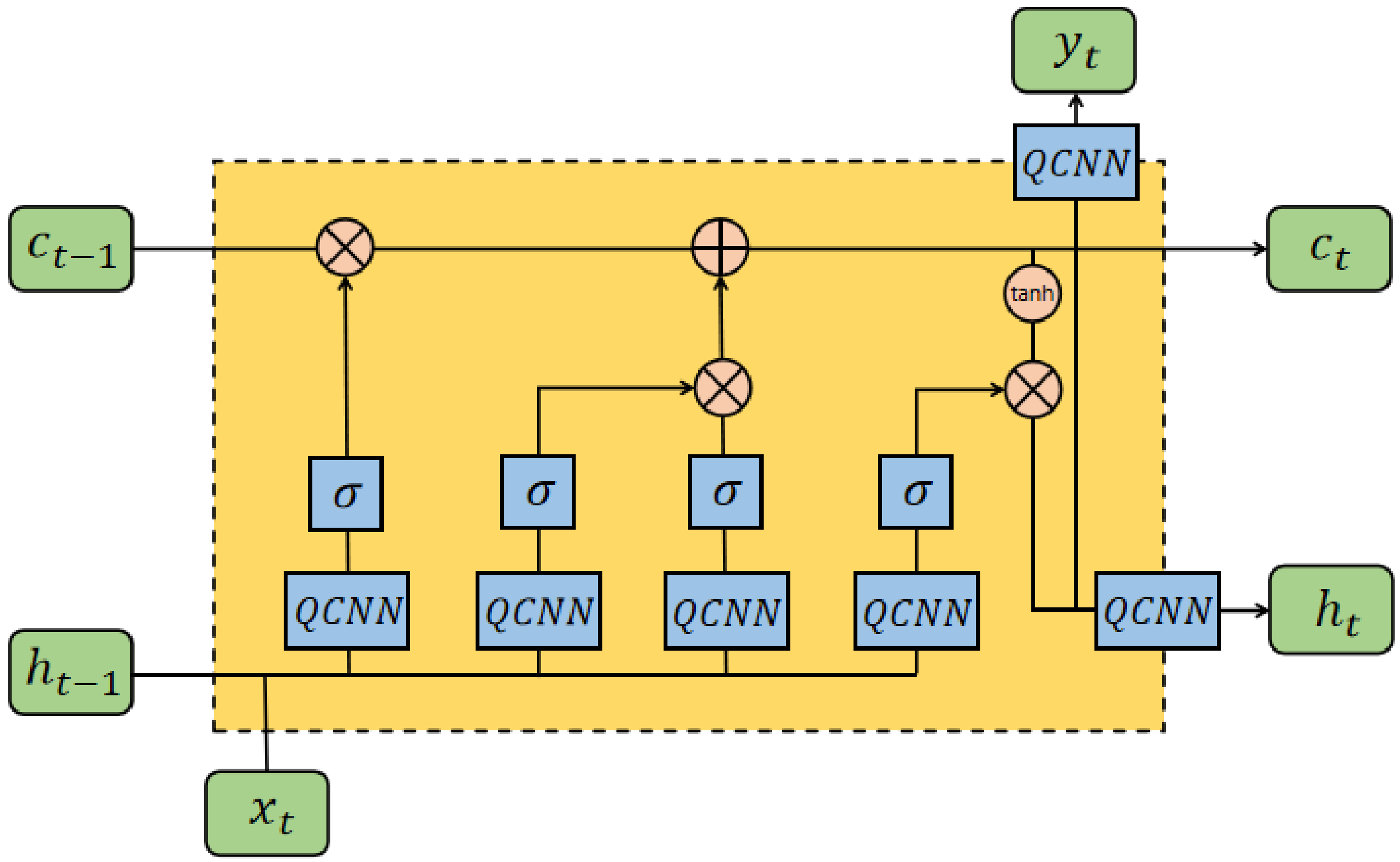
The main drawback of QLSTM in handling spatiotemporal data is that it uses quantum fully connected neural networks in both the input-to-state and state-to-state transitions, without encoding spatial information. Therefore, we replace the quantum fully connected circuit layer with a quantum convolution circuit layer, as illustrated in Figure 2. We treat each time step of the input sequence as an image. When the image sequence at a certain time enters the quantum LSTM unit, three types of control gates composed of quantum convolution circuits are applied to the sequence based on the actual situation. This is carried out to learn the spatial and temporal information contained in the sequence, thereby performing the modeling of the image sequence.

4.2. Quantum Convolutional Circuit Structure

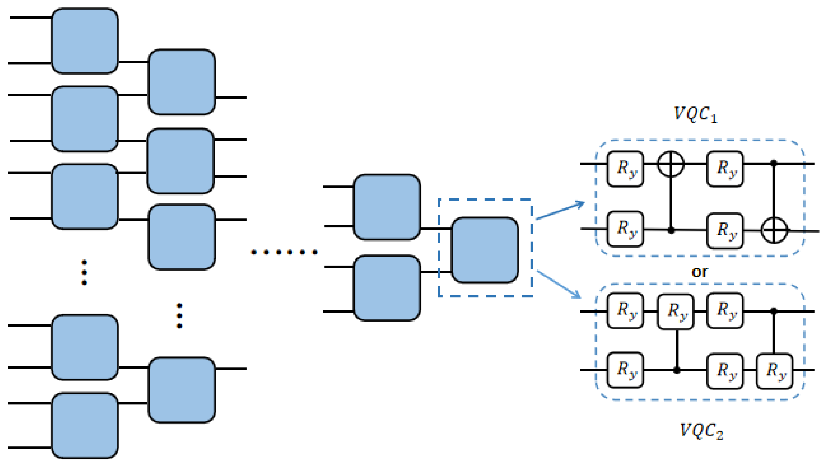
The approach adopted in this paper utilizes a hierarchical stacking method to design quantum circuits, gradually decreasing the number of qubits layer by layer in a tree-like structure. From a design perspective, the structure of this circuit is similar to that of a convolutional neural network. Through stacking and layer-by-layer qubit reduction operations, we fully exploit the parallelism of quantum computation while reducing the count of qubits and parameters, thus improving training efficiency. Additionally, the hierarchical structure offers flexibility and adjustability, allowing us to design and optimize according to specific problem requirements, adjust the number of layers, and select suitable gate operations and parameterization forms to improve the performance and convergence speed of the quantum algorithm.
The specific operations are illustrated in Figure 3. Firstly, we employ multiple sets of two-qubit VQC modules for combination, used to initialize the first layer of the circuit. Subsequently, we reduce the number of qubits in the next layer by discarding one qubit from each module’s output. In the next layer, we apply the two-qubit VQC module again to the remaining qubits and then discard half of them. This process is repeated until only one qubit remains, and finally, the average expectation value on the remaining qubits is measured. This design effectively avoids problems such as barren plateaus, enhancing the overall trainability and performance of the network. The V Q C 1 and V Q C 2 in the figure represent different circuit design structures. Different structures will lead to changes in the performance of the model, so it is necessary to design a circuit structure suitable for the current application scenario based on the actual situation. The details of this design will be discussed in Section 7.

5. Experiments

5.1. Experimental Setup

The dataset used in this experiment was the Moving-MNIST image dataset, with images having a resolution of 64 × 64 pixels. We selected 500 sequences from the dataset for training and 200 sequences for testing. The learning rate was set to 0.001, and the encoding method was amplitude encoding. The experiments were conducted on a Linux operating system, specifically Ubuntu 18.04.5 LTS, with GPU processing. The experimental code was implemented using Python 3, and the libraries chosen were PyTorch and PennyLane. PyTorch is an open source ML library that offers various ways to construct models and can utilize GPU acceleration for computing, making it suitable for large-scale data and complex models. PennyLane, on the other hand, is an open source quantum machine learning library specifically designed for gradient descent optimization in quantum computing. It provides interfaces based on popular machine learning frameworks such as PyTorch and TensorFlow and integrates code for simulating quantum noise, allowing users to develop and train noisy quantum machine learning models.
In our noise simulation experiment, we utilized noncoherent noise channels, namely (1) bit flip, (2) phase flip, (3) bit–phase flip, and (4) depolarizing. The Kraus operators corresponding to these four noise channels are represented by Equations (4)–(7) in sequence.
K 1 = 1 p 1 0 0 1 ,   and   K 2 = p 0 1 1 0
Equation (4) represents the Kraus operators for the bit flip channel, where p is the probability of a qubit undergoing a bit flip. The operator K 1 describes the case where no quantum state flip occurs, while the operator K 2 describes the case where an X gate is applied to the quantum state with a certain probability, controlling the quantum state to transition from state 0 to state 1 , or from state 1 to state 0 .
K 2 = p 1 0 0 1 ,   and   K 1 = 1 p 1 0 0 1
Equation (5) represents the Kraus operators for the phase flip channel, where the operator   K 2 describes the case where a Z gate is applied to the quantum state with a certain probability, controlling the quantum state to remain unchanged if it is in state 0   , or to transition from state 1 to state − 1 .
K 1 = 1 p 1 0 0 1 ,   and   K 2 = p 0 i i 0
Equation (6) represents the Kraus operators for the bit–phase flip channel, where the operator   K 2 describes the case where a Y gate is applied to the quantum state with a certain probability, controlling the quantum state to transition from state 0 to state i 1 , or from state 1 to state −i 0 .
K 1 = 1 3 p 2 1 0 0 1 ,   K 2 = p 2 1 0 0 1 K 3 = p 2 0 i i 0 ,   and   K 4 = p 2 1 0 0 1
Equation (7) represents the Kraus operators for the depolarizing channel. The depolarizing channel is characterized by the application of X, Y, and Z gates with equal probabilities on the quantum state.

5.2. Noiseless Simulations

In this section, we apply the proposed QConvLSTM framework to model the Moving-MNIST dataset. To compare the differences between classical and quantum learning, all model network hyperparameters were kept consistent. Firstly, based on the model architecture described in Section 4.1, we constructed the QConvLSTM model framework containing quantum convolutional layer operations. Additionally, during the model experimentation process, we adjusted and compared the model circuit’s number of layers to optimize the model’s performance. Ultimately, we chose the optimal setting with the circuit layers as 2.
In addition to ensuring the final training effectiveness of the model, it is also necessary to consider the available computing resources. Since we used the quantum simulator provided by the PennyLane platform in our experiment, the running speed of a real quantum computer could not be achieved. Therefore, to reduce the time complexity of training, we had to use circuits with as few qubits as possible. In this experiment, we used a two-layer four-qubit structure for the circuit. If using amplitude encoding, the maximum dimension of the input sequence that this circuit could accept was 16. However, since the Moving-MNIST dataset has a size of 64 × 64 pixels, it requires preprocessing to reduce the dimensionality of the sequences. We first reduced the original sequences to 64 × 16 using a fully connected layer and then split them into 64 batches to input into the circuit and encode them into quantum states.

5.3. Noisy Simulations

We simulated the scenario of noise by adding noise channels at each layer of the quantum convolutional network. Initially, based on the aforementioned experiments, we added noise channels at the end of the convolutional circuits in the QConvLSTM model, with the same type of noise channel added for each test. We conducted multiple tests using the same methodology as described in the previous experiment. Finally, we evaluated the robustness of our model to various types of noise during the training process by observing changes in performance metrics, thus assessing the noise robustness of the model. We utilized the four types of noise channels introduced in Section 5.1, namely bit flip, bit–phase flip, phase flip, and depolarizing noise. These four types of noise capture the impacts that most common noise sources may have.

6. Results

6.1. Noiseless

Table 1 presents the average results of all comparative models on each frame. We utilized evaluation metrics widely used by previous researchers: mean squared error (MSE) [47], structural similarity index measure (SSIM) [48], and learned perceptual image patch similarity (LPIPS) [49]. The distinctions among these metrics lie in the fact that the MSE estimates absolute pixel errors; the SSIM measures the similarity of structural information within spatial neighborhoods; and the LPIPS is based on deep features, which better align with human perception. Through these three types of metrics, we can comprehensively assess the sequence modeling ability of the models, where smaller MSE and LPIPS values indicate better performance, while the SSIM value is the opposite. Figure 4 provides the corresponding frame-by-frame comparison changes. By comparing multiple datasets, we can intuitively understand the performance differences among various LSTM variants. Regarding the MSE, firstly, by adding convolutional operations to LSTM, the ConvLSTM model reduced the mean MSE from 132.7 to 113.4 compared to the LSTM model. Secondly, by combining quantum algorithms with classical LSTM models, the QLSTM model further reduced the mean MSE to 87.2. Finally, our proposed QConvLSTM model further increased the mean MSE by 25.7% (from 87.2 to 64.8) by incorporating quantum convolutional networks. Additionally, the SSIM and LPIPS, respectively, improved by 2.1% and 14.5% over QLSTM. Therefore, it is concluded that, under the same parameters, the performance of the QConvLSTM model is superior to classical models and quantum models with quantum fully connected network structures.

6.2. Noisy

Table 2 shows the results of the simulation experiments for the four types of noise. The results indicate that the influence of these four types of noise on our QConvLSTM model can be neglected. The robustness of QConvLSTM to noise interference is determined by the special structure of the model. Firstly, the circuit depth used in our experiments is only two layers, and circuits with shallower depths are less prone to noise issues. Secondly, the LSTM unit with added convolutional operations can better extract features from the input data, enabling the network to adapt to and fit the influence of noise. Lastly, the introduced variational quantum algorithm can enhance the network’s ability to handle some nonlinear problems, assisting the network in better capturing and processing nonlinear information in the noise.

7. Discussion

As mentioned in Section 4.2, our circuit structure design adopts a hierarchical stacking approach. Therefore, we conducted multiple tests on the number of stacked layers in the circuit to find the optimal number of layers. As shown in Table 3, we tested the performance of the models under three scenarios. The single-layer circuit structure yielded the worst results, while the performance of the three-layer structure was slightly better than the two-layer structure. However, as the number of layers increased, both the computational complexity and time complexity grew exponentially, and an increase in network depth was more likely to lead to the emergence of noise. Therefore, we ultimately chose two layers as the number of layers for the experimental circuit.
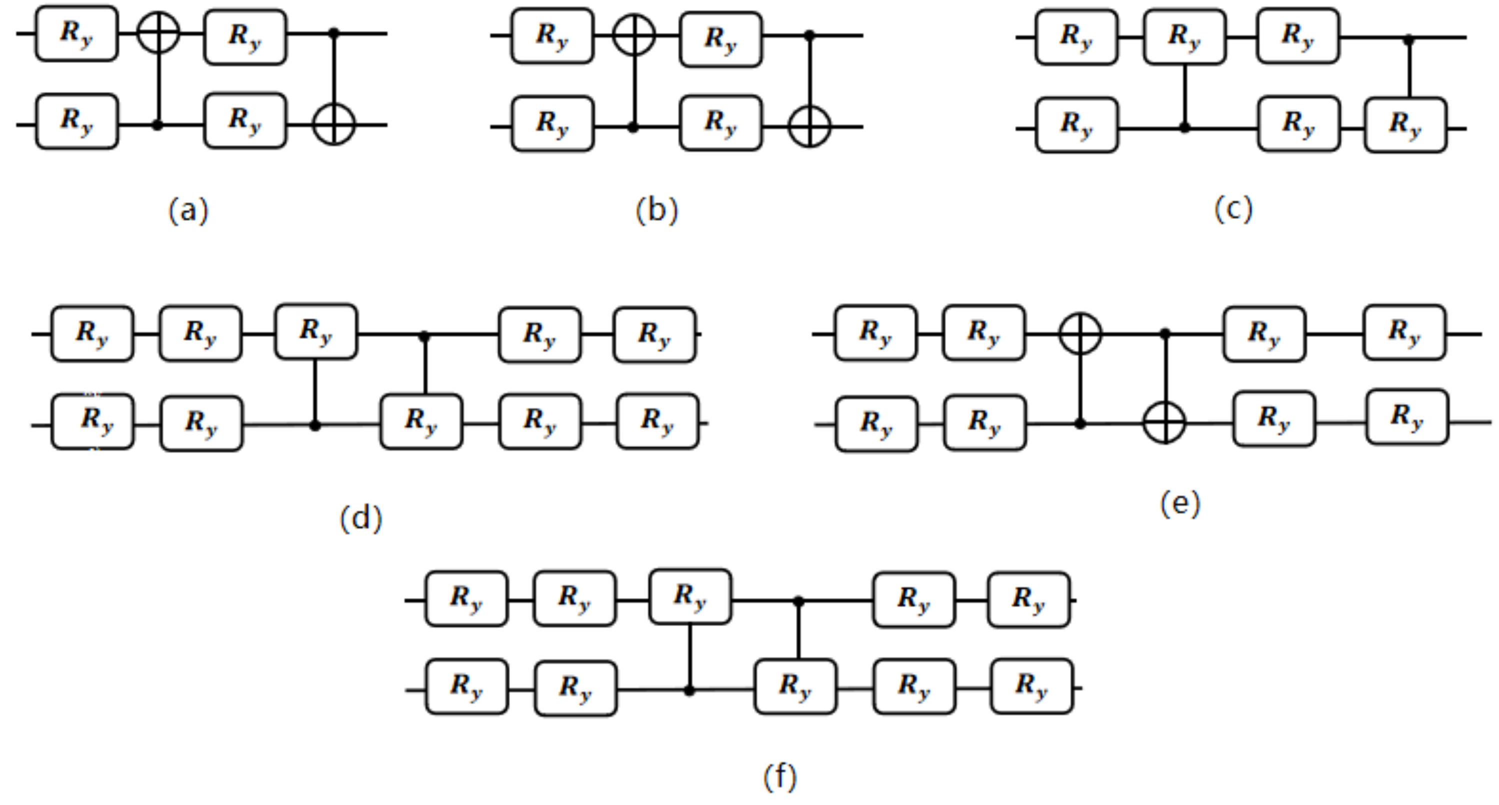
Typically, the structure of a quantum circuit can significantly impact the performance of the model. In the early stages of experimentation, we designed six types of circuit structures, as shown in Figure 5. We conducted comparative tests on these six types of circuits to select the one with the best performance as the final circuit for this experiment. According to the results in Table 4, the circuit labeled as (c) exhibited the best performance, surpassing the circuits with other structures. Therefore, we chose this structure as the final component of the model in this paper.

8. Conclusions

This paper introduces a novel QConvLSTM model that combines the advantages of quantum computing and convolutional networks on the basis of classical LSTM networks. This model not only improves the training efficiency but also enhances the model’s capability to extract spatial features. We first utilized the proposed model to predict the Moving-MNIST dataset and then evaluated the model’s performance based on loss value and accuracy. Experimental results demonstrate that, under the same parameters, the performance of QConvLSTM surpasses that of classical LSTM structures and QLSTM. Specifically, compared to QLSTM, QConvLSTM achieved a 25.7%, 2.1%, and 14.5% improvement in MSE, SSIM, and LPIPS, respectively. Furthermore, due to the hierarchical tree-like structure adopted by the circuit, we utilized fewer quantum bits during design, reduced network depth, decreased the overall parameter count of the model, and improved training efficiency. Finally, we demonstrate the robustness of QConvLSTM to the most common noise sources, which holds considerable practical significance in the era of NISQ computing.
The integration of quantum convolutional networks into classical LSTM provides new insights for future researchers in the study of quantum long short-term memory networks. The robustness of QConvLSTM to noise enables training on most current NISQ devices. However, due to device limitations, the experiments in this work were confined to low-resolution image data. In future work, we aim to extend our model to high-resolution image tasks and attempt to reconstruct the control gate structure within LSTM units using structurally diverse quantum neural networks. Furthermore, our research on noise robustness remains incomplete. In the future, we will expand our study to include noise factors such as phase damping, amplitude damping, and depolarization damping.

Author Contributions

Methodology, C.Z.; Formal analysis, Y.C.; Writing—original draft, Z.X.; Writing—review & editing, W.Y. All authors have read and agreed to the published version of the manuscript.

Funding

This research was funded by the Natural Science Foundation of China, grant number 62071240, and the Natural Science Foundation of Jiangsu Province, grant number BK20231142.

Institutional Review Board Statement

Not applicable.

Informed Consent Statement

Not applicable.

Data Availability Statement

All the data are publicly available. The dataset used for this study is the Moving-MNIST.

Conflicts of Interest

The authors declare no conflicts of interest.

References

  1. Hochreiter, S.; Schmidhuber, J. Long short-term memory. Neural Comput. 1997, 9, 1735–1780. [Google Scholar] [CrossRef] [PubMed]
  2. Karpathy, A.; Fei-Fei, L. Deep visual-semantic alignments for generating image descriptions. In Proceedings of the IEEE Conference on Computer Vision and Pattern Recognition (CVPR), Boston, MA, USA, 7–12 June 2015. [Google Scholar]
  3. Pascanu, R.; Mikolov, T.; Bengio, Y. On the difficulty of training recurrent neural networks. In Proceedings of the 30th International Conference on Machine Learning, PMLR, Atlanta, GA, USA, 16–21 June 2013; pp. 1310–1318. [Google Scholar]
  4. Sutskever, I.; Vinyals, O.; Le, Q.V. Sequence to sequence learning with neural networks. In Proceedings of the Advances in Neural Information Processing Systems 27 (NIPS 2014), Montreal, QC, Canada, 8–13 December 2014; pp. 3104–3112. [Google Scholar]
  5. Bengio, Y.; Goodfellow, I.; Courville, A. Deep Learning; MIT Press: Cambridge, MA, USA, 2015. [Google Scholar]
  6. Srivastava, N.; Mansimov, E.; Salakhudinov, R. Unsupervised learning of video representations using lstms. In Proceedings of the 32nd International Conference on Machine Learning, PMLR, Lille, France, 6–11 July 2015. [Google Scholar]
  7. Xu, K.; Ba, J.; Kiros, R.; Cho, K.; Courville, A.; Salakhudinov, R.; Bengio, Y. Show, attend and tell: Neural image caption generation with visual attention. In Proceedings of the 32nd International Conference on Machine Learning, Lille, France, 6–11 July 2015. [Google Scholar]
  8. Gers, F.A.; Schmidhuber, E. LSTM recurrent networks learn simple context-free and context-sensitive languages. IEEE Trans. Neural Netw. 2001, 12, 1333–1340. [Google Scholar] [CrossRef] [PubMed]
  9. Eck, D.; Schmidhuber, J. A first look at music composition using lstm recurrent neural networks. Ist. Dalle Molle Studi Sull Intell. Artif. 2002, 103, 48–56. [Google Scholar]
  10. Wang, S.; Jiang, J. Learning natural language inference with LSTM. arXiv 2015, arXiv:1512.08849. [Google Scholar]
  11. Monner, D.; Reggia, J.A. A generalized LSTM-like training algorithm for second-order recurrent neural networks. Neural Netw. 2012, 25, 70–83. [Google Scholar] [CrossRef] [PubMed]
  12. Krause, B.; Lu, L.; Murray, I.; Renals, S. Multiplicative LSTM for sequence modelling. arXiv 2016, arXiv:1609.07959. [Google Scholar]
  13. Chen, Q.; Zhu, X.; Ling, Z.; Wei, S.; Jiang, H.; Inkpen, D. Enhanced LSTM for natural language inference. arXiv 2016, arXiv:1609.06038. [Google Scholar]
  14. Cao, Z.; Zhu, Y.; Sun, Z.; Wang, M.; Zheng, Y.; Xiong, P.; Tian, L. Improving prediction accuracy in LSTM network model for aircraft testing flight data. In Proceedings of the 2018 IEEE International Conference on Smart Cloud (SmartCloud), New York, NY, USA, 21–23 September 2018. [Google Scholar]
  15. Wang, Y.; Zhu, S.; Li, C. Research on multistep time series prediction based on LSTM. In Proceedings of the 2019 3rd International Conference on Electronic Information Technology and Computer Engineering (EITCE), Xiamen, China, 18–20 October 2019. [Google Scholar]
  16. Edholm, G.; Zuo, X. A Comparison between Aconventional LSTM Network and Agrid LSTM Network Applied on Speech Recognition; KTH Royal Institute of Technology: Stockholm, Sweden, 2018. [Google Scholar]
  17. Schuld, M.; Sinayskiy, I.; Petruccione, F. An introduction to quantum machine learning. Contemp. Phys. 2015, 56, 172–185. [Google Scholar] [CrossRef]
  18. Lloyd, S.; Mohseni, M.; Rebentrost, P. Quantum algorithms for supervised and unsupervised machine learning. arXiv 2013, arXiv:1307.0411. [Google Scholar]
  19. Havenstein, C.; Thomas, D.; Chandrasekaran, S. Comparisons of performance between quantum and classical machine learning. SMU Data Sci. Rev. 2018, 1, 11. [Google Scholar]
  20. Chen, S.Y.C.; Yoo, S.; Fang, Y.L.L. Quantum long short-term memory. In Proceedings of the ICASSP 2022—2022 IEEE International Conference on Acoustics, Speech and Signal Processing (ICASSP), Singapore, 23–27 May 2022. [Google Scholar]
  21. Yulita, I.N.; Purwani, S.; Rosadi, R.; Awangga, R.M. A quantization of deep belief networks for long short-term memory in sleep stage detection. In Proceedings of the 2017 International Conference on Advanced Informatics, Concepts, Theory, and Applications (ICAICTA), Denpasar, Indonesia, 16–18 August 2017. [Google Scholar]
  22. Khan, S.Z.; Muzammil, N.; Zaidi, S.M.H.; Aljohani, A.J.; Khan, H.; Ghafoor, S. Quantum long short-term memory (qlstm) vs. classical lstm in time series forecasting: A comparative study in solar power forecasting. arXiv 2023, arXiv:2310.17032. [Google Scholar]
  23. Nielsen, M.A.; Chuang, I.L. Quantum Computation and Quantum Information; Cambridge University Press: Cambridge, UK, 2010. [Google Scholar]
  24. Torlai, G.; Melko, R.G. Machine-learning quantum states in the NISQ era. Annu. Rev. Condens. Matter Phys. 2020, 11, 325–344. [Google Scholar] [CrossRef]
  25. Huang, H.L.; Xu, X.Y.; Guo, C.; Tian, G.; Wei, S.J.; Sun, X.; Long, G.L. Near-term quantum computing techniques: Variational quantum algorithms, error mitigation, circuit compilation, benchmarking and classical simulation. Sci. China Phys. Mech. Astron. 2023, 66, 250302. [Google Scholar] [CrossRef]
  26. Cerezo, M.; Arrasmith, A.; Babbush, R.; Benjamin, S.C.; Endo, S.; Fujii, K.; Coles, P.J. Variational quantum algorithms. Nat. Rev. Phys. 2021, 3, 625–644. [Google Scholar] [CrossRef]
  27. Lubasch, M.; Joo, J.; Moinier, P.; Kiffner, M.; Jaksch, D. Variational quantum algorithms for nonlinear problems. Phys. Rev. A 2020, 101, 010301. [Google Scholar] [CrossRef]
  28. Jones, T.; Endo, S.; McArdle, S.; Yuan, X.; Benjamin, S.C. Variational quantum algorithms for discovering Hamiltonian spectra. Phys. Rev. A 2019, 99, 062304. [Google Scholar] [CrossRef]
  29. Zhao, A.; Tranter, A.; Kirby, W.M.; Ung, S.F.; Miyake, A.; Love, P.J. Measurement reduction in variational quantum algorithms. Phys. Rev. A 2020, 101, 062322. [Google Scholar] [CrossRef]
  30. Bonet-Monroig, X.; Wang, H.; Vermetten, D.; Senjean, B.; Moussa, C.; Bäck, T.; O’Brien, T.E. Performance comparison of optimization methods on variational quantum algorithms. Phys. Rev. A 2023, 107, 032407. [Google Scholar] [CrossRef]
  31. Sakib, S.N. SM Nazmuz Sakib’s Quantum LSTM Model for Rainfall Forecasting; OSF Preprints: Peoria, IL, USA, 2023. [Google Scholar]
  32. Beaudoin, C.; Kundu, S.; Topaloglu, R.O.; Ghosh, S. Quantum Machine Learning for Material Synthesis and Hardware Security. In Proceedings of the 41st IEEE/ACM International Conference on Computer-Aided Design, San Diego, CA, USA, 30 October–3 November 2022. [Google Scholar]
  33. Parcollet, T.; Morchid, M.; Linarès, G.; De Mori, R. Bidirectional quaternion long short-term memory recurrent neural networks for speech recognition. In Proceedings of the 2019 IEEE International Conference on Acoustics, Speech and Signal Processing (ICASSP 2019), Brighton, UK, 12–17 May 2019. [Google Scholar]
  34. Shi, X.; Chen, Z.; Wang, H.; Yeung, D.Y.; Wong, W.K.; Woo, W.C. Convolutional LSTM network: A machine learning approach for precipitation nowcasting. In Advances in Neural Information Processing Systems; Curran Associates Inc.: Witless Bay, NL, Canada, 2015; p. 28. [Google Scholar]
  35. Mateo-García, G.; Adsuara, J.E.; Pérez-Suay, A.; Gómez-Chova, L. Convolutional long short-term memory network for multitemporal cloud detection over landmarks. In Proceedings of the 2019 IEEE International Geoscience and Remote Sensing Symposium (IGARSS 2019), Yokohama, Japan, 28 July–2 August 2019. [Google Scholar]
  36. Kosana, V.; Madasthu, S.; Teeparthi, K. A novel hybrid framework for wind speed forecasting using autoencoder-based convolutional long short-term memory network. Int. Trans. Electr. Energy Syst. 2021, 31, e13072. [Google Scholar] [CrossRef]
  37. Sudhakaran, S.; Lanz, O. Learning to detect violent videos using convolutional long short-term memory. In Proceedings of the 2017 14th IEEE International Conference on Advanced Video and Signal Based Surveillance (AVSS), Lecce, Italy, 29 August–1 September 2017. [Google Scholar]
  38. Paiva, E.; Paim, A.; Ebecken, N. Convolutional neural networks and long short-term memory networks for textual classification of information access requests. IEEE Lat. Am. Trans. 2021, 19, 826–833. [Google Scholar] [CrossRef]
  39. Gandhi, U.D.; Malarvizhi Kumar, P.; Chandra Babu, G.; Karthick, G. Sentiment analysis on twitter data by using convolutional neural network (CNN) and long short term memory (LSTM). In Wireless Personal Communications; Springer: Berlin/Heidelberg, Germany, 2021; pp. 1–10. [Google Scholar]
  40. LaRose, R.; Coyle, B. Robust data encodings for quantum classifiers. Phys. Rev. A 2020, 102, 032420. [Google Scholar] [CrossRef]
  41. Gao, S.; Yang, Y.G. New quantum algorithm for visual tracking. Phys. A Stat. Mech. Its Appl. 2023, 615, 128587. [Google Scholar] [CrossRef]
  42. Huang, S.Y.; An, W.J.; Zhang, D.S.; Zhou, N.R. Image classification and adversarial robustness analysis based on hybrid quantum–classical convolutional neural network. Opt. Commun. 2023, 533, 129287. [Google Scholar] [CrossRef]
  43. Bar, N.F.; Yetis, H.; Karakose, M. An efficient and scalable variational quantum circuits approach for deep reinforcement learning. Quantum Inf. Process. 2023, 22, 300. [Google Scholar] [CrossRef]
  44. Kim, R. Implementing a Hybrid Quantum-Classical Neural Network by Utilizing a Variational Quantum Circuit for Detection of Dementia. arXiv 2023, arXiv:2301.12505. [Google Scholar]
  45. Gong, L.H.; Pei, J.J.; Zhang, T.F.; Zhou, N.R. Quantum convolutional neural network based on variational quantum circuits. Opt. Commun. 2024, 550, 129993. [Google Scholar] [CrossRef]
  46. Ren, W.; Li, Z.; Huang, Y.; Guo, R.; Feng, L.; Li, H.; Li, X. Quantum generative adversarial networks for learning and loading quantum image in noisy environment. Mod. Phys. Lett. B 2021, 35, 2150360. [Google Scholar] [CrossRef]
  47. Error, M.S. Mean Squared Error; Springer: Boston, MA, USA, 2010; p. 653. [Google Scholar]
  48. Jia, X.; De Brabandere, B.; Tuytelaars, T.; Gool, L.V. Dynamic filter networks. In Proceedings of the Advances in Neural Information Processing Systems 29 (NIPS 2016), Barcelona, Spain, 5–10 December 2016; pp. 667–675. [Google Scholar]
  49. Ronneberger, O.; Fischer, P.; Brox, T. U-net: Convolutional networks for biomedical image segmentation. In Proceedings of the International Conference on Medical Image Computing and Computer-Assisted Intervention, Munich, Germany, 5–9 October 2015; pp. 234–241. [Google Scholar]
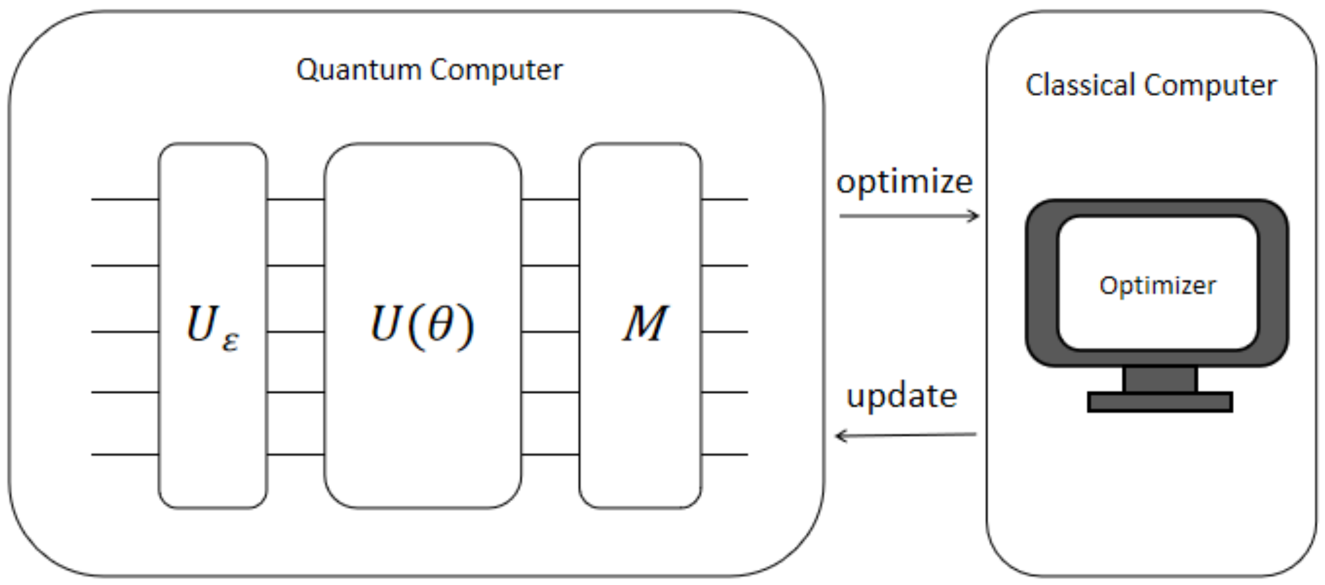
Figure 1. Parameter update process in a VQC. The entire process occurs simultaneously in both quantum and classical environments. Variational operations are performed on a quantum computer, while parameter optimization operations are carried out on a classical computer.
Information 15 00175 g001
Figure 2. The basic framework of the LSTM unit based on quantum convolutional neural networks. σ represents the sigmoid function, while the tanh block denotes the hyperbolic tangent activation function. x t   represents the input at time t, h t represents the hidden state, c t represents the cell state, and y t represents the output. and , respectively, denote addition and multiplication operations.
Information 15 00175 g002
Figure 3. A quantum convolutional circuit based on a hierarchical tree-like structure. The entire circuit is composed of multiple two-qubit VQC modules concatenated together, with each column representing a layer of the circuit. Each blue square represents a VQC module, which can be flexibly constructed according to specific requirements.
Information 15 00175 g003
Figure 4. Frame-by-frame results of the Moving-MNIST test set generated by models trained on the training set: (a) MSE; (b) SSIM; (c) LPIPS.
Information 15 00175 g004
Figure 5. Structural design of VQC: (af) represent the design schemes of a single VQC module in the quantum convolution circuit based on a hierarchical tree structure.
Information 15 00175 g005
Table 1. Average performance of different models on 10 prediction time steps.
ModelMSESSIMLPIPS
( )( )( )
LSTM132.70.6870.174
ConvLSTM113.40.7580.162
QLSTM87.20.8430.095
QConvLSTM64.80.8610.083
Table 2. Performance metric comparison of QConvLSTM in different noise environments.
EnvironmentMSESSIMLPIPS
( )( )( )
Noiseless64.80.8610.083
Bit flip64.10.8590.084
Phase flip65.00.8570.081
Bit–phase flip65.90.8530.085
Depolarizing66.10.8500.089
Table 3. Performance comparison of circuit structures with different numbers of layers.
LayersMSESSIMLPIPS
( )( )( )
1 Layer67.50.7830.092
2 Layers64.80.8610.083
3 Layers64.90.8630.081
Table 4. Comparison of the impact of different VQC structures on training effectiveness.
StructureMSESSIMLPIPS
( )( ) ( )
VQC (a)65.90.8050.095
VQC (b)65.20.8320.089
VQC (c)64.80.8610.083
VQC (d)65.30.8460.092
VQC (e)65.70.8270.094
VQC (f)65.40.8360.092
Disclaimer/Publisher’s Note: The statements, opinions and data contained in all publications are solely those of the individual author(s) and contributor(s) and not of MDPI and/or the editor(s). MDPI and/or the editor(s) disclaim responsibility for any injury to people or property resulting from any ideas, methods, instructions or products referred to in the content.