A Convolutional Deep Neural Network Approach to Predict Autism Spectrum Disorder Based on Eye-Tracking Scan Paths

Abstract

Autism spectrum disorder (ASD) is a developmental disorder that encompasses difficulties in communication (both verbal and non-verbal), social skills, and repetitive behaviors. The diagnosis of autism spectrum disorder typically involves specialized procedures and techniques, which can be time-consuming and expensive. The accuracy and efficiency of the diagnosis depend on the expertise of the specialists and the diagnostic methods employed. To address the growing need for early, rapid, cost-effective, and accurate diagnosis of autism spectrum disorder, there has been a search for advanced smart methods that can automatically classify the disorder. Machine learning offers sophisticated techniques for building automated classifiers that can be utilized by users and clinicians to enhance accuracy and efficiency in diagnosis. Eye-tracking scan paths have emerged as a tool increasingly used in autism spectrum disorder clinics. This methodology examines attentional processes by quantitatively measuring eye movements. Its precision, ease of use, and cost-effectiveness make it a promising platform for developing biomarkers for use in clinical trials for autism spectrum disorder. The detection of autism spectrum disorder can be achieved by observing the atypical visual attention patterns of children with the disorder compared to typically developing children. This study proposes a deep learning model, known as T-CNN-Autism Spectrum Disorder (T-CNN-ASD), that utilizes eye-tracking scans to classify participants into ASD and typical development (TD) groups. The proposed model consists of two hidden layers with 300 and 150 neurons, respectively, and underwent 10 rounds of cross-validation with a dropout rate of 20%. In the testing phase, the model achieved an accuracy of 95.59%, surpassing the accuracy of other machine learning algorithms such as random forest (RF), decision tree (DT), K-Nearest Neighbors (KNN), and multi-layer perceptron (MLP). Furthermore, the proposed model demonstrated superior performance when compared to the findings reported in previous studies. The results demonstrate that the proposed model can accurately classify children with ASD from those with TD without human intervention.

1. Introduction

The prevalence of autism spectrum disorder (ASD) is on the rise globally. Currently, approximately one in 68 children has been diagnosed with ASD [1]. ASD is a neurodevelopmental disorder that impacts the behavioral and cognitive abilities of children, including communication and social interaction [2]. People with ASD have difficulties in social communication and interaction, such as struggles with social–emotional reciprocity, non-verbal communication, and building and understanding relationships [3]. Previous research on ASD has examined the unique obstacles in understanding both spoken and non-spoken signals of communication. These obstacles encompass challenges in monitoring eye movements, and recognizing and replicating gestures and facial expressions, as well as grasping language pragmatics and verbal interactions. Diagnosing ASD presents a complex and rigorous challenge, focusing on examining interactive behaviors in diagnostic conversations. This examination involves evaluating how the person being assessed aligns their verbal and non-verbal actions with their conversation partner (interpersonal coordination), and also observing the frequency and characteristics of their repetitive behaviors (intrapersonal coordination). The expert needs to interact with the child, be mindful of their own conversational style, and make diagnostic notes according to their observations. Examining the level of interactional coordination in various conversation settings during autism diagnosis could offer valuable information about an individual’s ability to adjust behavior across different conversational contexts and its impact on diagnostic results. However, many studies have concentrated on behaviors at the individual utterance level or used overall statistics at the conversation level. As a result, the real-time dynamic elements of coordination in conversations are not adequately captured [4].

In numerous countries globally, parents often request a formal assessment and diagnosis primarily due to delayed initiation of communication and language or insufficient linguistic abilities in comparison to children of a similar age. This emphasizes that a considerable number of children with ASD encounter difficulties in developing language. Proficiency in language consistently proves to be a reliable indicator of social and academic achievements, emphasizing the significance of giving priority to language assistance when formulating intervention objectives for children with ASD [5]. As children diagnosed with ASD mature, some may make efforts to understand the anticipated behaviors and suitable language usage, although this may not be uniform across all contexts. Nevertheless, they frequently face difficulties in grasping the deeper implications in dialogues, resulting in literal understandings and struggles in recognizing indirect messages like sarcasm or minor deceptions. Clear and specific instructions are necessary for their understanding, as individuals with ASD might find it hard to deduce meanings without explicit guidance, despite possessing good verbal communication abilities. Nonetheless, they commonly experience difficulties in utilizing language appropriately in social environments [3].

The severity of symptoms and the impact of ASD differ from one case to another. In recent times, numerous research studies have been carried out with the aim of enhancing the quality of life for individuals with ASD. These studies suggest that early detection and intervention can have a significant impact on the diagnosis of ASD, leading to reduced costs for both individuals and society as a whole [6]. Children with autism typically display symptoms early in life, but their diagnosis is often delayed until they reach school age. Several research studies have highlighted various factors that contribute to this delay, such as limited resources in rural areas and low-income families, the effectiveness of ongoing pediatric care, a shortage of specialized referrals, and parents’ awareness of autism spectrum disorder (ASD) [7]. Diagnosing ASD is a difficult task because of its intricate characteristics and diverse range of symptoms [2]. Moreover, the identification of ASD poses challenges due to the necessity of specialized professionals utilizing methods such as observation, interviews, and questionnaires [1]. Specialist physicians in a clinical setting are usually responsible for the official diagnosis of ASD. They utilize a clinical judgment procedure and rely on observable and measurable behavioral indicators. However, the current diagnostic tools are time-consuming due to the extensive number of items that need to be checked by the specialist. These tools also rely on static human-embedded rules. As a result, there is a need to modify the coding and behavior of ASD clinical tools in order to classify cases more efficiently [1]. Despite the significant financial investment in the advancement of detection methods, clinical treatments have not yielded successful results thus far. The primary challenges contributing to these issues include clinicians’ limited access to adequate data and their inability to conduct thorough data analysis [8]. Furthermore, autism is a diverse condition with various manifestations. A standardized diagnosis approach that encompasses all cases and allows for self-treatment by specialists is lacking. Each specialist relies on their own expertise and experience to diagnose autism spectrum disorder (ASD), resulting in inconsistencies and a lack of reliability in the diagnostic process [9]. Consequently, there is a demand for advanced intelligent techniques that can swiftly and automatically classify ASD [1].

Eye-tracking technology plays a significant role in the diagnosis of autism spectrum disorder (ASD) by analyzing visual patterns [10]. Typically, an eye-tracking device consists of a high-resolution digital camera and an intelligent algorithm that precisely detects eye gaze coordinates while individuals view videos or images. The eye gaze data obtained from this technology provide valuable insights into the challenges faced by individuals with ASD in social interactions, enabling interventions to be customized according to their unique requirements [7]. One way to enhance our knowledge about the use of eye-tracking biomarkers in distinguishing different subsets of individuals with autism spectrum disorder (ASD) is to examine the potential impact of highly comorbid psychiatric conditions such as Attention Deficit Hyperactivity Disorder (ADHD), anxiety, and mood disorder. By doing so, we can gain a better understanding of how these conditions may affect the ability to identify specific populations within a clinical setting. For instance, research has shown that children who have both ASD and ADHD tend to display shorter fixation durations on faces when viewing static low-complexity social stimuli, as compared to children with ASD only and those with typical development (TD) [11].

Based on research findings, eye-tracking data have been found to serve as a biomarker for the early detection of autism spectrum disorder (ASD) in children [7]. Biomarkers, also known as biological markers, are measurable and objective indicators that provide information about a patient’s observable biological condition. Bodily fluids or soft tissue biopsies are commonly utilized to evaluate the effectiveness of treatment for a disease or medical condition. By examining eye movements, researchers have discovered that an atypical preference for geometric images can serve as an early indicator of a specific subtype of autism spectrum disorder, which is linked to more severe symptoms [11]. Compared to other types of data, the analysis of biomarkers on images is often more challenging. This is because biomarkers are not only defined by numerical values but also by their spatial relationship to one another. The precision and reliability of biomarker analysis are significantly impacted by the resolution of the image. This is due to the fact that the numerical values representing biomarker indicators in the image are crucial. In cases where there is spatial variation among these indicators within tissues or organisms, the distribution of digital values in the image will differ. Therefore, specific methods are required to accurately capture and measure the spatial correlations among these indicators. However, the complex nature of biological images often necessitates the involvement of human experts in annotating these biomarkers. Unfortunately, this process is time-consuming, labor-intensive, subjective, and prone to errors. To address these limitations, various software applications have been developed to automate data classification and assist healthcare professionals. The advent of machine learning techniques, particularly neural networks, has revolutionized this field [8]. Eye tracking has the potential to be utilized in routine clinical settings for the purpose of aiding specialists in the diagnosis of autism spectrum disorder (ASD) [12]. The results of a study indicate that eye-tracking data can significantly assist clinicians in efficiently and accurately screening for autism [7].

The CNN-based architecture was selected for this problem due to its impressive performance and accuracy in computer vision problems and image classification compared to other deep neural network architectures. It can autonomously and adaptively learn features from signals and images. A CNN is widely used in image-processing tasks including object detection, object recognition, anomaly detection, and segmentation. One of the main advantages of CNNs over previous models is its ability to extract relevant features from input images without human intervention [7]. In this study, we introduce a model called Tuned-Convolutional Neural Network-Autism Spectrum Disorder (T-CNN-ASD) that can classify eye-tracking scan path images of children with ASD and typical development (TD) without the need for human intervention. Additionally, various image-processing techniques are employed to extract the most significant features from eye-tracking scan path images of individuals with ASD. The dataset used in this research, which consists of 59 children with an average age of around 8 years, was obtained from the participation of these individuals [13]. A total of 547 images were used in the study by Carette et al. (2019) [10]. The authors then proceeded to construct the T-CNN-ASD model for the classification of eye-tracking scan path images. To improve the model’s performance, various architectures were fine-tuned using different optimizers to determine the optimal optimizer and model parameters. These parameters included kernel sizes, stride, dropout, number of batches, number of epochs, and pooling parameter, all aimed at improving the accuracy of the model. The performance of the T-CNN-ASD model will be compared to that of popular classification techniques such as random forest, decision tree, K-Nearest Neighbors (KNN), and multi-layer perceptron (MLP). Furthermore, the proposed model will be compared to previous studies in the literature. Figure 1 provides a summary of the research methodology.

This paper is structured as follows. In Section 1, an overview of ASD and the commonly employed methods for classifying ASD is provided. Section 2 presents the previous research conducted in this area. The proposed methodology is discussed in Section 3. Section 4 presents the experimental results. Finally, Section 5 concludes the findings of this research and provides suggestions for future work.

2. Related Works

Numerous investigations have been conducted on the utilization of machine learning (ML) techniques for detecting autism through eye tracking. One such study, described in [6], involved the presentation of a speaking face and the analysis of children’s gaze patterns. The researchers discovered that individuals with ASD tend to have shorter periods of fixation on the eyes, mouth, nose, body, person, face, and outer person in comparison to those without ASD. The authors utilized SVM as a classification method to distinguish between individuals with autism spectrum disorder (ASD) and typically developing (TD) individuals. They based their classification on the ratios of fixation times for all areas of interest (AOIs). The outcomes of their model classification are as follows: an accuracy rate of 85.1%, a sensitivity rate of 86.5%, and a specificity rate of 83.8%. In [14], the researchers introduced a technique for categorizing various degrees of ASD by utilizing eye gaze patterns and demographic descriptors like age. They used multiple ML classifiers to classify ASD. The researchers examined the utilization of two different sets of attributes. The initial collection includes features that were created manually and unprocessed gaze data. This combination achieved an accuracy rate of 90.83% when using both the PART and C4.5 classifiers. The second group consists of gaze pattern-based features that were manually created. These features achieved an accuracy rate of 93.45% when a random forest was used. Furthermore, the researchers calculated the Pearson correlation coefficient to determine the correlation between each feature and the classification output. It was observed that the average classification accuracy decreased when age was excluded as a feature in all tested classifiers. In addition, Vabalas et al. [15] utilized ML techniques along with eye-tracking and motion data to distinguish between autistic and non-autistic adults. They integrated both motion and eye-tracking data to improve the accuracy of their classification. The authors discovered that the kinematic and eye movement datasets contained more features than the samples. To address this issue, they employed the ‘wrapped t-test’ method, which combines features from both the filter and wrapper methods. By selecting a subset of features that yielded the highest classification performance, they eliminated certain portions of the features. Their model achieved an accuracy of 73% in predicting the diagnosis based on kinematic characteristics, 70% accuracy using features of eye movement, and 78% accuracy when combining both sets of features.

Several investigations have employed artificial neural networks (ANNs) to categorize instances of AD. For instance, Carette et al. [10] explored the fusion of eye-tracking technology with ANNs to aid in the identification of ASD. At first, non-neural network methods were employed. The accuracy attained by this group of models was satisfactory. Following that, the model was tested with different artificial neural network (ANN) architectures. Based on the findings, the single-layer model consisting of 200 neurons produces the highest accuracy. The authors of [16] conducted research on the visual attention of children with ASD when observing human faces. They utilized deep neural networks (DNNs) to extract semantic characteristics. The feature maps for autism spectrum disorder (ASD) exhibit distinct characteristics when observing human faces in comparison to individuals without ASD. These feature maps are subsequently combined with the features obtained from CASNet. In their study, the researchers compared CASNet with six other deep learning models and discovered that CASNet outperformed all of them in every scenario. In their work [17], the authors introduced a method for classifying children with TD and ASD using the eye gaze scan paths. They utilized a combination of convolutional neural networks (CNNs) and long short-term memory (LSTM) networks. The CNN-LSTM model was employed to extract features from the saliency maps and the sequence of fixation locations in the scan path. Moreover, the pretrained prediction model SalGAN was utilized for data preprocessing and to generate the network input. The proposed model achieved an accuracy of 74.22% on the validation dataset.

Our research stands out from prior studies in the following aspects: First, we addressed the issue of working with a dataset containing a small number of images without utilizing augmentation. Whereas many earlier studies depended on augmenting image data to improve outcomes, we maintained the original image count and achieved superior performance. Additionally, while numerous prior research works tested different machine learning algorithms to identify the most effective one, our study utilized CNNs. We carefully adjusted the parameters of the CNN model and offered explanations for the superior outcomes. This methodology enabled us to attain peak performance without resorting to image augmentation.

3. Proposed Methodology

Clinicians often face challenges and time constraints when diagnosing autism spectrum disorder (ASD) due to the wide range of symptoms associated with the condition. The heterogeneity of ASD symptoms leads to distinct variations within specific subgroups. Unfortunately, there is currently no reliable method to measure the diversity of autism symptoms in children, making it difficult to plan targeted interventions for smaller groups. However, research has shown a strong correlation between ASD heterogeneity and the complexity of eye-tracking data. Therefore, by utilizing advanced algorithms based on convolutional neural networks (CNNs), machine learning models could be used to quantify the variations in ASD symptoms, enabling accurate classification of ASD severity based on eye-tracking data [7]. The aim of this study is to develop an enhanced convolutional deep neural network for the identification of autism using eye-tracking scan path images. The methodology consists of several stages, including image processing, cross-validation, the creation of a T-CNN-ASD model, fine-tuning of model parameters, and evaluation of the model. The architecture of the proposed methodology is depicted in Figure 2.

3.1. Dataset Collection

The study made use of the public dataset mentioned in [13]. This dataset was employed to carry out experiments assessing the efficacy of eye-tracking technology within the realm of autism spectrum disorder (ASD). It comprises data from a study involving 59 children, with 29 diagnosed with ASD and the remaining 30 being typically developing children averaging around 8 years of age. A cohort of typically developing (TD) children was enlisted from various French schools in the Hauts-de-France region. All procedures involving human participants were conducted following the ethical standards set by the institutional and/or national research committee, as well as in compliance with the 1964 Helsinki Declaration and its subsequent amendments or similar ethical standards. The children with ASD were evaluated in specialized clinics, and the level of autism in each child was gauged using the Childhood Autism Rating Scale (CARS).

Table 1. Information about the participants.

Number of Participants	59
Gender Distribution (M/F)	38 (64%)/21 (36%)
Number of Non-ASD	30
Number of ASD-Diagnosed	29
Age (Mean/Median) years	7.88/8.1
CARS (Mean/Median)	32.97/34.50

presents a summary of the participants’ statistics [10].

The dataset underwent several stages of processing. At first, participants viewed a collection of videos containing particular scenarios aimed at prompting eye movement on the screen. Participants could be seated on their own or on their parent’s lap at approximately 60 cm distance from the display screen. The experiments were conducted in a quiet room at the University premises. Additionally, physical white barriers were used to reduce visual distractions. These videos were carefully created to include visually attractive components, especially appealing to children, like colorful balloons and animated characters. Moreover, the positioning of these components changed during the study. Some videos also included a live host who interacted verbally with the child, trying to guide their focus towards both seen and hidden elements. It is important to mention that all interactions and dialogues took place in French, the participants’ mother tongue.

The eye tracking function was performed using the SMI Experiment Center Software remote eye tracker (Red-m 250 Hz). The motion path of the eye was then transformed into images. The resulting visualizations comprised a dataset of 547 images, with 328 images corresponding to participants without ASD and 219 images corresponding to participants with ASD. Furthermore, all images had a default size of $640\times 480$ pixels.

As mentioned earlier, the field of autism spectrum disorder (ASD) has placed particular emphasis on the utilization of eye tracking technology due to the consistent identification of gaze abnormalities as a characteristic feature of autism in general [10]. The divergence in the eye tracking patterns between children with ASD and typically developing (TD) children is illustrated in Figure 3.

3.2. Stage of Image Processing

Image processing refers to the application of various operations on an image in order to improve its quality or extract valuable information from it, prior to the implementation of other algorithms. Numerous image-processing techniques can be utilized, including but not limited to image resizing, geometric transformation, and conversion of color images to grayscale images [18].

The computer analyzes the image by treating it as a collection of pixels. The resolution of the image is determined by its height, width, and dimension, which are represented in the format $h\times w\times d$ (where h is the height, w is the width, and d is the dimension). For instance, an image with a resolution of $3\times 3\times 3$ corresponds to a matrix of Red, Green, and Blue (RGB) values. Conversely, an image with a resolution of $3\times 3\times 1$ represents a grayscale image in the form of a matrix.

The CNN model can process the pixel representation of image matrices. By doing so, it can detect edges, colors, and shapes in the images, enabling image recognition. The model is capable of performing tasks such as classification and object detection within an image. However, training the CNN model using raw images may lead to lower accuracy in classification.

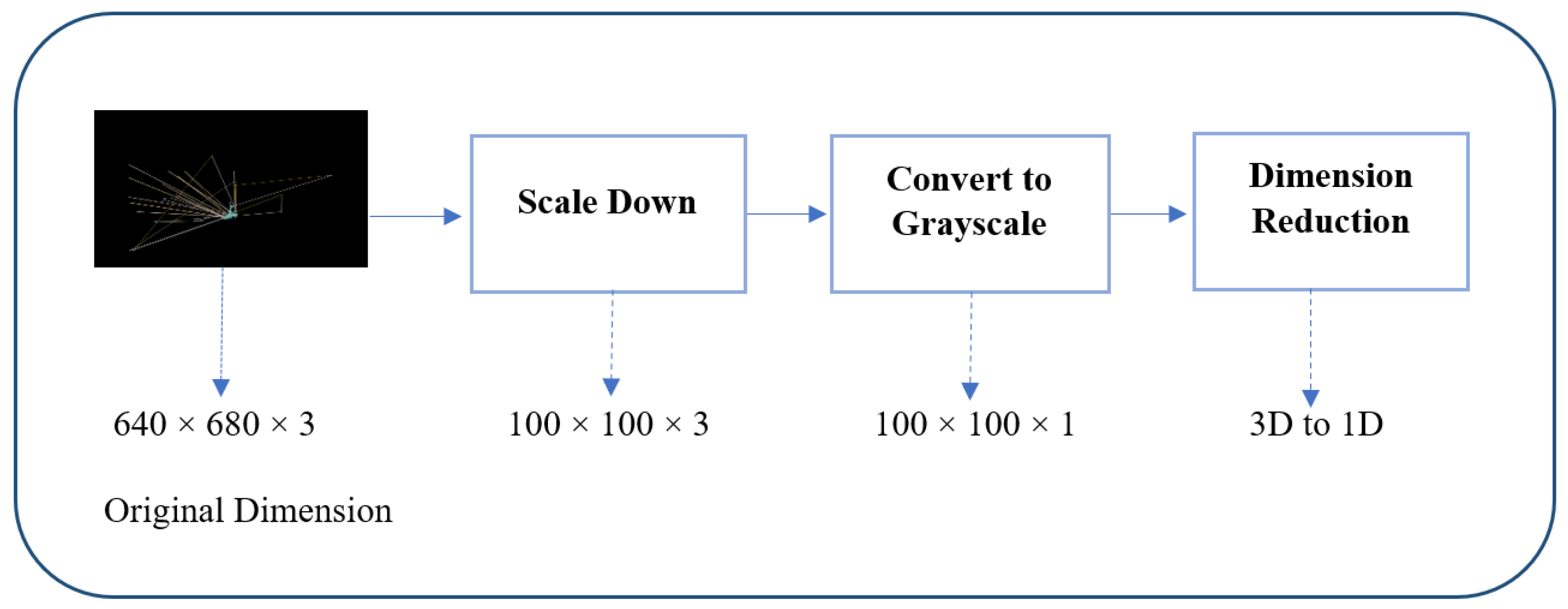
Furthermore, the process of preprocessing is regarded as a crucial step in accelerating the training of models [18]. As a result, various processing techniques were employed to enhance the model’s resilience and enhance the performance of the T-CNN-ASD. The image-processing techniques applied to the images in this paper are depicted in Figure 4.

3.2.1. Reducing the Size of Images

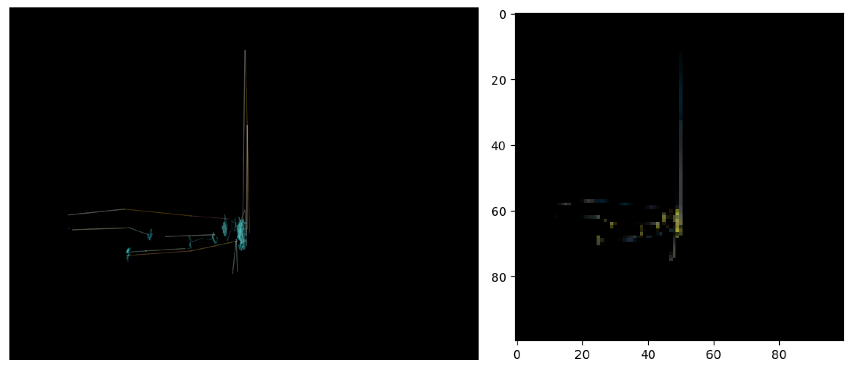
Image data are fed in batches to train T-CNN-ASD. A batch of images requires that all images be of the same size. Therefore, all images fed into the model must have the same height and width. Therefore, rescaling images is needed to fit the image size to the feature maps that are used [18]. All images were scaled down to 100 × 100 with the colors of the images being RGB. Their resizing would not cause much loss of information since most images contained a large blank space of unused pixels [10]. Thus, the dimensions of the image become 100 × 100 × 3. Figure 5 shows the scaling of a sample image.

3.2.2. Grayscale Image Conversion

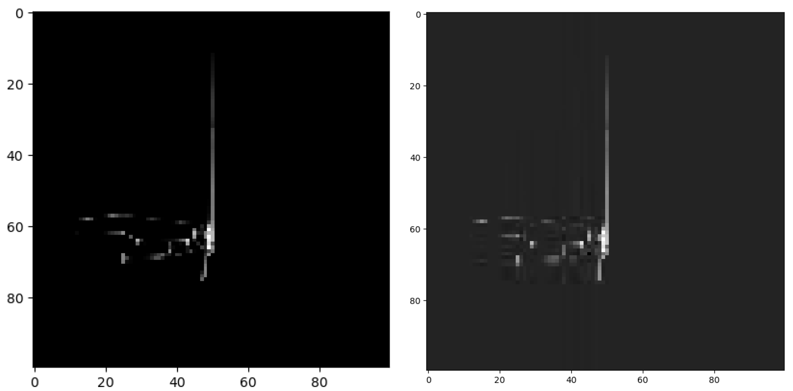
In this stage, the images are transformed into grayscale format to simplify the computations and reduce space usage. Color images contain more intricate information that may not be necessary and occupy more space compared to grayscale images. Figure 6 illustrates the process of converting the image to grayscale [19].

3.2.3. Reduction in Dimensions

Dimensionality reduction methods aim to convert a high-dimensional dataset into a lower-dimensional representation, while preserving the essential information of the original data. This process facilitates the analysis, processing, and visualization of the data [20]. This research utilizes large images with high-dimensional features. To handle this, dimensionality reduction is performed prior to using the images for training the T-CNN-ASD. The images are compressed by converting them from a 3D representation to a 1D representation. This reduction in dimensionality aids in extracting important latent features from the data, enabling the T-CNN-ASD to focus on relevant features and avoid dealing with irrelevant ones. Figure 7 illustrates the process of converting the image to 1D.

3.3. Cross-Validation

Cross-validation is a method used to assess the performance of predictive models. It involves splitting the dataset into training and testing sets in order to evaluate the model. The main purpose of its usage is to assess ML models [21]. Model generalization is achieved through the use of cross-validation, specifically K-fold cross-validation. In this approach, the dataset is divided into K groups, with K representing the number of groups. During each iteration, K-1 groups are used for training the model, while the remaining group is used for testing. This process is repeated K times to prevent overfitting during training [22]. Typically, the value of K is set to 5 or 10, as recommended in various studies in the field of applied machine learning [23].

3.4. T-CNN-ASD Model

Image classification is a task within the field of computer vision, as mentioned in the study by Filchev et al. (2020) [24]. There are various methods available for image classification, with the most common ones being CNNs. CNNs are well-suited for image classification due to their ability to effectively reduce the dimensionality of the image, which is necessary given the large number of parameters involved. The process of using CNNs involves extracting features from the image in order to identify patterns within the dataset [25].

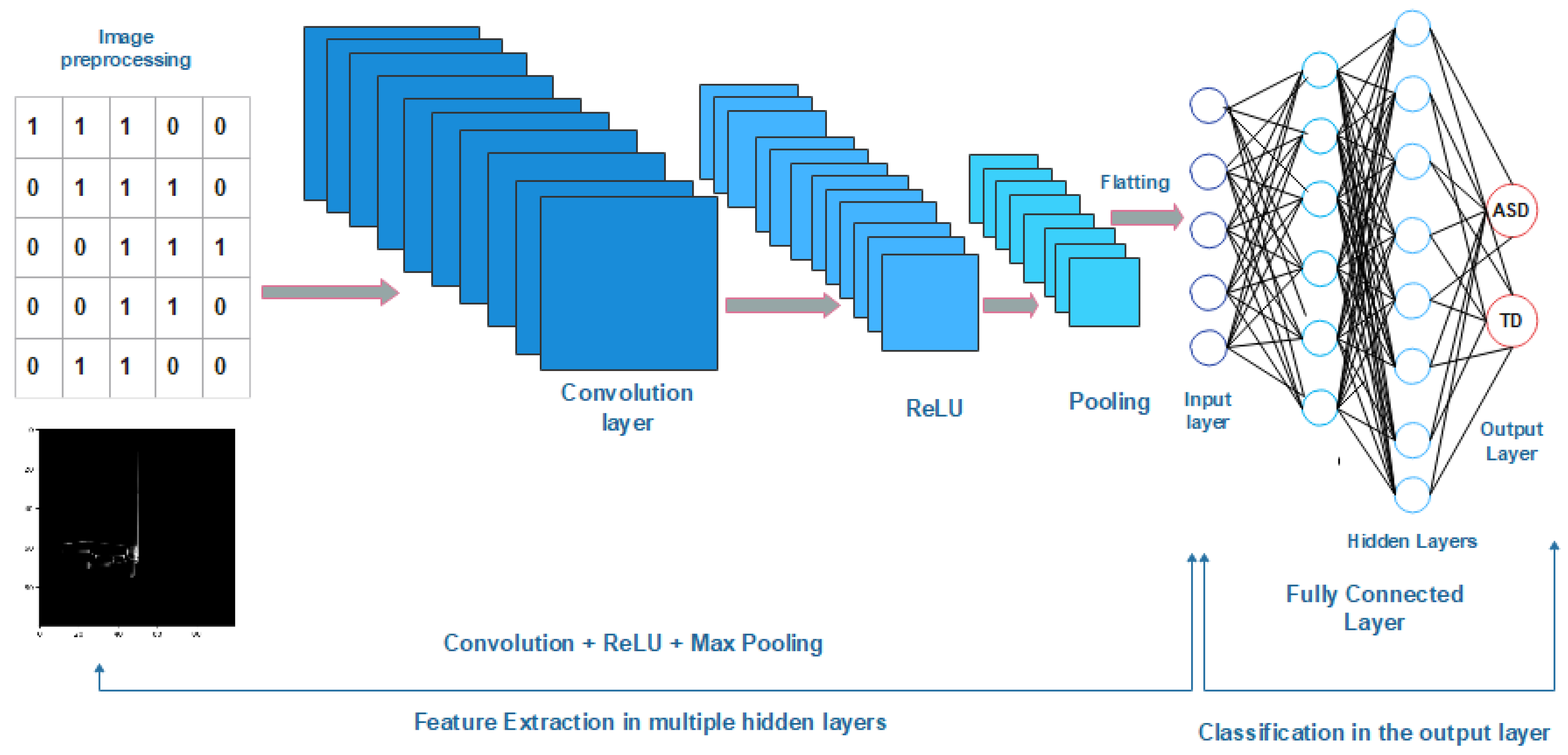
The T-CNN-ASD model is composed of different layers, including the input layer, the output layer, and multiple hidden layers. These hidden layers are made up of convolutional layers, ReLU activation function, pooling layers, and fully connected layers. The model can have a combination of convolutional and pooling layers, with the number of hidden layers varying depending on the specific problem being addressed. In some cases, a single hidden layer is sufficient, while in others, multiple layers are needed, followed by one or more fully connected layers [7]. The process of going from input data to output through these layers is referred to as forward propagations, as mentioned in [26]. The T-CNN-ASD structure, as depicted in Figure 8, is designed to implement this process. In this structure, the input image undergoes convolution layers and ReLU activation to extract features, followed by downsampling through pooling layers. Subsequently, the extracted features are fed into a fully connected layer for the classification of the image as ASD or TD.

The subsequent sections provide an overview of the primary components of the T-CNN-ASD architecture:

• The initial layer of T-CNN-ASD is referred to as the input layer. It accepts images as input, resizes them, and subsequently forwards them to subsequent layers for the purpose of extracting features.
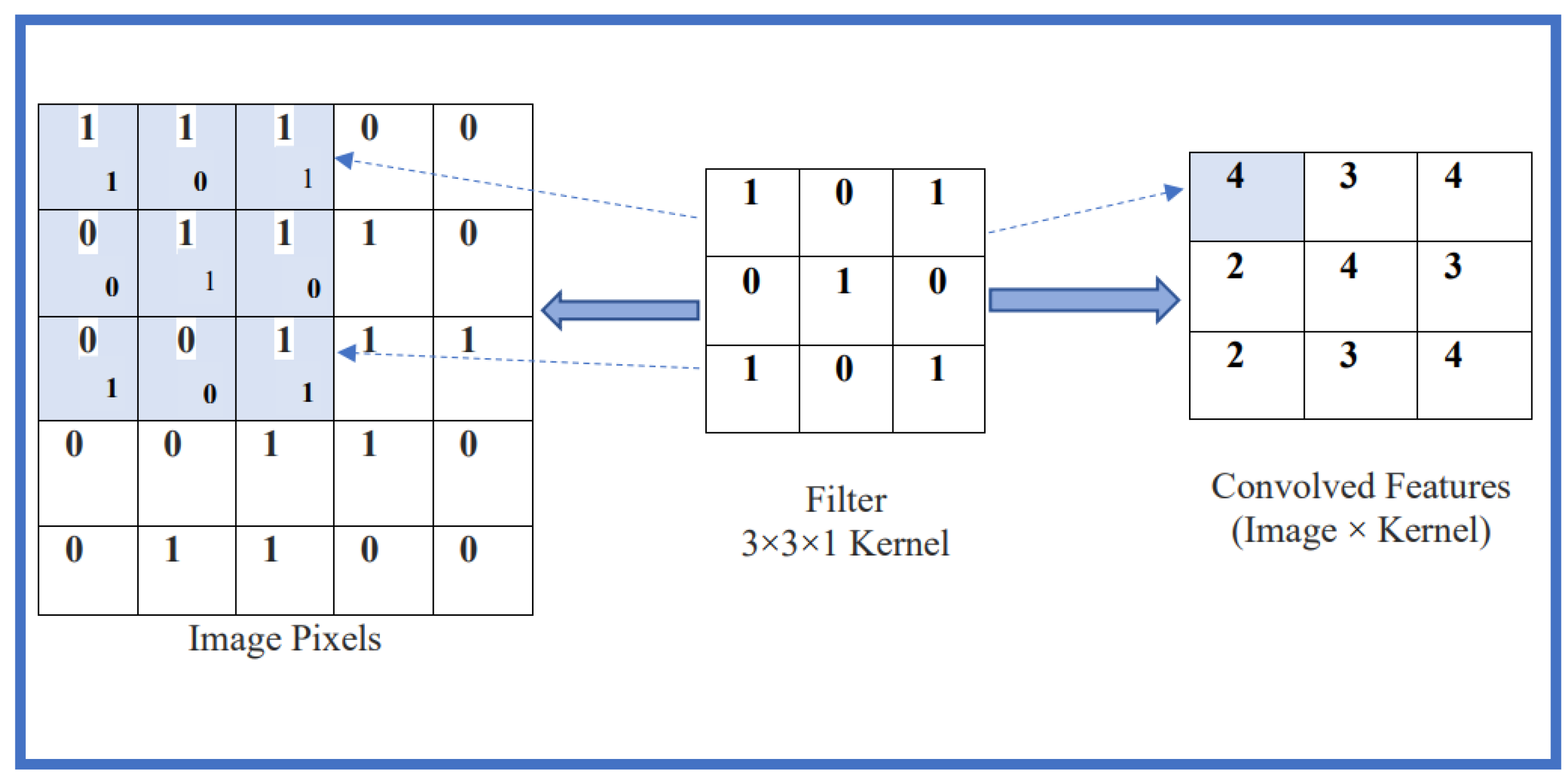
• The convolution layer is responsible for extracting spatial and temporal features from an input image through the process of convolution. It consists of multiple filters or kernels that perform convolution on the entire image. To configure the convolution layer, important parameters such as the number and size of the kernels need to be set. In the T-CNN-ASD model, each image is represented as an array of pixel values. These pixel values are then passed to the convolutional layer. Within this layer, the kernels move across receptive fields in the input image, searching for specific cues like edges, colors, and curves. Figure 9 provides a visual representation of this process [27].
  T-CNN-ASD is composed of multiple convolutional layers, generating numerous feature maps in the input layer. These maps are then utilized as the input for subsequent layers to detect a wide range of features for learning purposes.
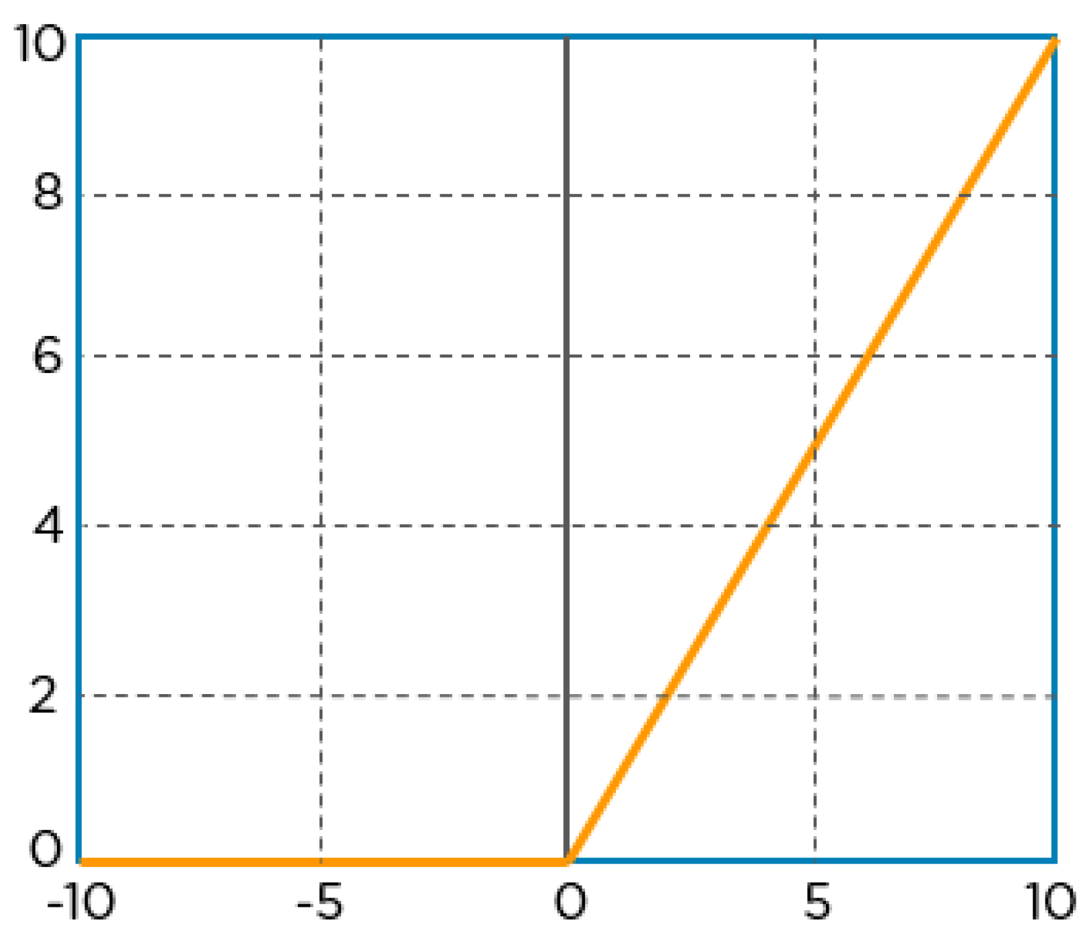
• The Rectified Linear Unit (ReLU) is a linear function that processes the input directly if it is positive, and if it is negative, it transforms it to 0. This activation function has been widely used in various neural network models due to its improved performance and ease of training. It can be represented mathematically as f(x) = max(0, x) [28]. In the context of T-CNN-ASD, the ReLU helps maintain mathematical stability by preventing learned values from getting stuck near 0 or approaching infinity. The process of the ReLU is illustrated in Figure 10.
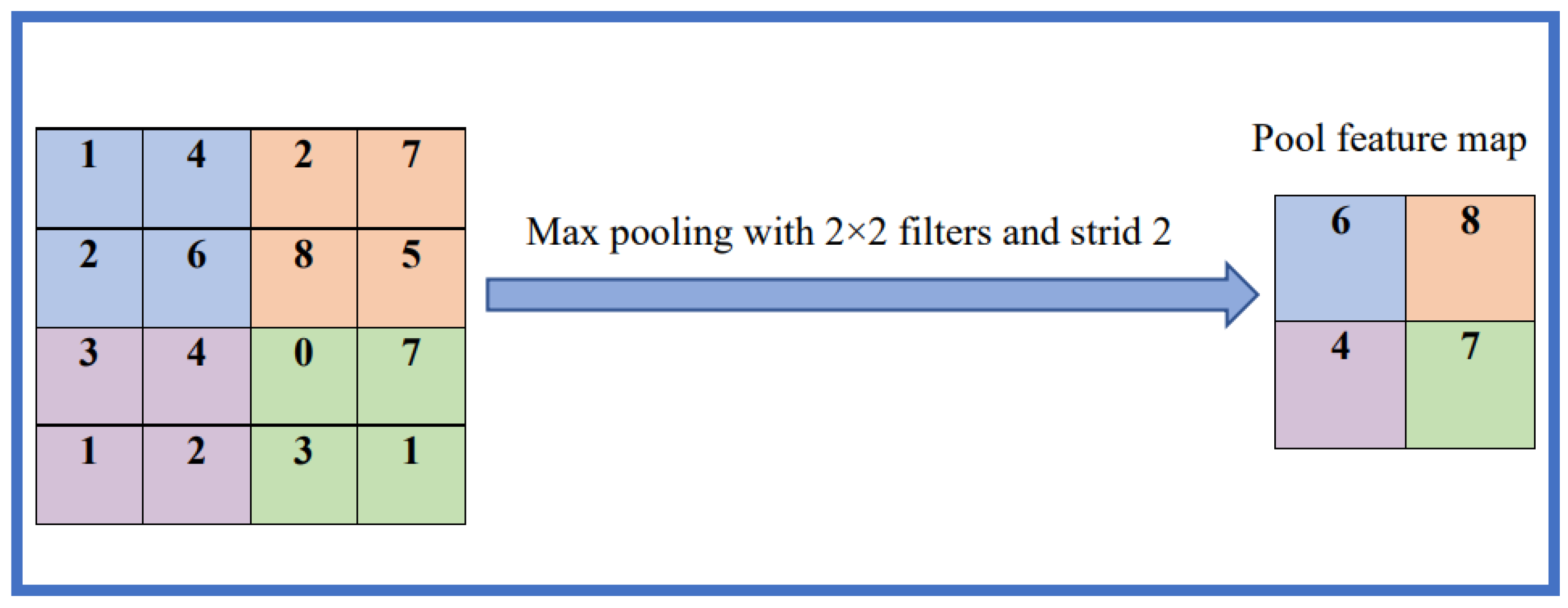
• Pooling Layer: The feature sets obtained from the previous layer are forwarded to the pooling layer. The purpose of this layer is to decrease the size of large images while still preserving the crucial information. In this study, both maximum and average pooling techniques were employed. These techniques involve extracting patches from the input feature maps. Max pooling selects the maximum value within each area, which represents the most prominent feature, while disregarding the remaining values. For this research, a maximum pooling method with a filter size of $2\times 2$ and a stride of 2 was utilized. The max-pooling layer is illustrated in Figure 11.
  The process of average pooling involves computing the average value of each patch in the feature map. In other words, a 2 × 2 square in the feature map is reduced to its average value [6]. Figure 12 illustrates the operation of average pooling.
  A pooling layer provides a downsampling operation, which reduces the internal dimensionality of the feature maps. It is of note that there is no learnable parameter in any of the pooling layers, whereas filter size, stride, and padding are hyperparameters in pooling operations. Unlike height and width, the depth dimension of the feature maps remains unchanged [26].
• The Fully Connected Layer is considered the last layer in a network. Its purpose is to take the high-level filtered images and convert them into categories or classes with corresponding labels. The output feature maps from the final convolution or pooling layer are typically flattened, meaning they are transformed into a one-dimensional array of numbers. These flattened feature maps are then connected to one or more fully connected layers. In these layers, each input is connected to every output through a weight that can be measured [29]. Once the features extracted by the convolution layers and downsampled by the pooling layers are generated, a subset of fully connected layers is used to map them to the final output of the network [29].

3.5. Tuning the Hyperparameters of T-CNN-ASD

Despite the impressive performance of deep network methods in noise reduction tasks, many of these methods encounter issues with vanishing or exploding gradients when the network architecture is excessively deep [30]. Consequently, parameter adjustments are needed to achieve optimal performance. Additionally, accurate prediction in different datasets necessitates the use of distinct sets of hyperparameters.

The presence of a multitude of hyperparameters creates a challenge for users in selecting the most appropriate ones. Determining the optimal number of layers, neurons, or optimizer for all datasets is not a straightforward task. It is crucial to fine-tune these parameters to identify the most suitable set for constructing a model based on a particular dataset. The subsequent items will delve into the hyperparameters that have undergone tuning.

• The architecture of the CNN-ASD model can be optimized by tuning its hyperparameters. One important hyperparameter to consider is the number of neurons in each hidden layer. The optimal number of neurons should be chosen based on the complexity of the problem being solved. In this study, we experiment with different numbers of neurons to identify the value that yields the highest accuracy. It is worth noting that the accuracy of the neural network can also be influenced by the number of layers. The selection of layers plays a crucial role in determining the performance of the prediction model. Using too few layers may lead to underfitting, while employing too many layers may result in overfitting. Hence, tuning the number of layers can lead to improved results.
• Optimizing primary hyperparameters in convolutional and pooling layers:
  • Kernel/Filter Size: The size of the kernel refers to the width × height of the filter mask. Various kernel sizes were employed to determine the optimal kernel size that yielded the highest level of accuracy.
  • Stride and Padding: The stride refers to the number of steps the filter moves in each step during convolution. It determines the number of pixels that are skipped while traversing the input horizontally and vertically after each element-wise multiplication of the input weights with those of the filter [26]. Figure 13 illustrates the stride parameter.
    Padding is employed to maintain the output size equal to the input size. The output size is smaller compared to the input size. Padding is a technique utilized to append zero-filled columns and rows in order to preserve the spatial dimensions after convolution. This can potentially enhance performance by preserving information at the boundaries. It is employed to ensure that the output dimension matches the input dimension [26].
  • Dropout: When the dataset is small in size, it is possible for overfitting to occur. This means that while the training results may be satisfactory, the test results are not as good. The reason for this is that the model is not able to accurately generalize to data that it has not encountered during training. If the model is unable to effectively generalize to unseen data, it will struggle to perform the intended classification or prediction tasks. To address this issue, dropout is employed as a means of reducing overfitting. Dropout is a regularization technique that decreases the likelihood of overfitting by randomly dropping out neurons during each epoch (or during each batch when using a batch approach). When a unit is dropped, the corresponding neuron is temporarily removed from the network, along with all of its incoming and outgoing connections [31], as illustrated in Figure 14.
  • Batch Size (BS): The batch size refers to the number of samples that the network will process simultaneously. This parameter plays a crucial role in enhancing the training process, particularly when fine-tuning is involved [32].
  • Epochs refer to the number of times the learning algorithm processes the entire training dataset. It is a hyperparameter that determines how many passes the algorithm will make over the data. Each epoch allows every sample in the training dataset to update the internal model parameters. An epoch consists of one or more batches. The rationale behind using epochs is to ensure that the network has the opportunity to observe previous data and adjust the model parameters, preventing bias towards the most recent data points during training [33].
• Optimizers are responsible for modifying the learning rate and weights of neurons in a neural network in order to minimize the loss function or maximize the accuracy. During the training process, the weights of the neural network are randomly initialized and then updated in each epoch to improve the overall accuracy. The loss function is used to calculate the error by comparing the output of the training data with the actual data at each epoch, and the weights are adjusted accordingly [34]. The optimizers employed include the adaptive moment estimate (Adam) optimizer, stochastic gradient descent (SGD) optimizer, Adadelta optimizer, Root Mean Square Propagation (RMSprop) optimizer, AdaMax optimizer, and Nesterov Accelerated Adam (Nadam) optimizer.

3.6. Model Evaluation

Once the image processing and implementation of the T-CNN-ASD model for image classification have been completed, the next step is to determine the evaluation method for the autism classification task. Various performance metrics are utilized to evaluate different machine learning algorithms. One commonly used measure is accuracy, which can be defined as an evaluation metric for classification problems by employing a confusion matrix to compare different machine learning classifiers. Given that the dataset is balanced, accuracy is chosen as the metric to assess the model’s performance. Accuracy is calculated as the ratio of correctly identified examples in all classes, as shown in Equation (1). Given that the research pertains to the medical field, it is essential to incorporate the following metrics: sensitivity, indicated by Equation (2), specificity, represented by Equation (3), and the F1 score, illustrated in Equation (4).

$$Accuracy=\frac{TP+TN}{TP+TN+FP+FN}$$

(1)

$$Sensitivity=\frac{TP}{TP+FN}$$

(2)

$$Specificity=\frac{TN}{TN+FP}$$

(3)

$$F1Score=\frac{2\ast (Sensitivity\ast Specificity)}{Sensitivity+Specificity}$$

(4)

where TP = True Positives, TN = True Negatives, FP = False Positives, and FN = False Negatives.

Furthermore, to assess the model’s performance, the mean accuracy is compared to that of other models such as MLP, random forest, decision tree, and KNN.

4. Experiments and Results

This section provides a discussion of the experiments conducted and the corresponding results.

4.1. Environment Setup

The experiments were carried out using a machine with the following specifications: Intel Core i7 10th GEN processor, 64-bit operating system, X64-based processor, 16 GB RAM, NVIDIA GeForce MX230 graphics card, and 1TB secondary storage. The machine ran on Windows 10 Pro. Preprocessing steps and T-CNN-ASD were carried out using Python IDLE 3.6.8. The main Python packages used were Keras (based on Tensorflow), OpenCV, Sklearn, and Matplotlib. To standardize the images, they were scaled down to 100 × 100 pixels and converted to grayscale using various image-processing techniques. Additionally, the images were compressed by converting them from 3D to 1D. The results were obtained without using augmented images. The training dataset consisted of 410 images (75% for training), while the test dataset had 137 images (25% for testing).

4.2. Sensitivity Analysis

In order to achieve optimal performance and obtain the desired outcomes, the proposed model necessitates the adjustment of multiple hyperparameters.

In this research, different configurations of neurons and layers were utilized, alongside the tuning of hyperparameters, to find the best accuracy. Various architectures were examined by adjusting different model parameters, with the goal of identifying the most efficient architecture with the optimal parameters.

• Results of Different Kernel/Filter Size: The training of the model involved 10 rounds of cross-validation, with each round consisting of 100 epochs and a dropout rate of 20%.

  Table 2. T-CNN-ASD accuracy with different kernel size.

  Number of Neurons	Hidden Layers	The Kernel Size
  		3	6	9
  50	Single layer	92.95	93.69	93.25
  100		93.87	93.79	93.05
  200		93.51	94.07	83.98
  300		93.97	93.44	87.12
  400		92.87	94.16	93.14
  500		93.61	94.13	84.58
  600		93.33	89.87	83.86
  80, 40	Two layers	94.69	91.93	93.35
  100, 50		94.87	93.80	91.04
  200, 100		94.52	90.59	86.93
  300, 150		95.59	85.23	81.71
  400, 200		94.96	93.06	87.24
  500, 250		93.59	85.82	81.59

  Bold values represent the best results.

  displays the accuracy achieved for various kernel sizes.
  The T-CNN-ASD model reached a peak accuracy of 95.59% by employing two layers with 300 and 150 neurons, respectively. The kernel size for these layers was set to 3.
• Results of Different Stride: This paper trained the model using 10 rounds of cross-validation, with 100 epochs and a 20% dropout rate. The kernel size used was 3, and the stride initially set to 1 but later changed to 2. The results can be seen in

  Table 3. T-CNN-ASD accuracy with different stride.

  Number of Neurons	Hidden Layers	Stride
  		1	2
  50	Single layer	92.95	92.61
  100		93.87	92.71
  200		93.51	92.87
  300		93.97	92.31
  400		92.87	93.69
  500		93.61	93.13
  600		93.33	93.60
  80, 40	Two layers	94.69	93.05
  100, 50		94.87	94.06
  200, 100		94.52	93.60
  300, 150		95.59	94.14
  400, 200		94.96	93.23
  500, 250		93.59	93.96

  Bold values represent the best results.

  .
  By including two layers with 300 and 150 neurons and a stride of 1, the T-CNN-ASD model achieved an outstanding performance of 95.59%.
• Pooling Layers: The training of the model was conducted using 10 rounds of cross-validation. Each round consisted of 100 epochs with a dropout rate of 20%. The kernel size used was 3. After applying max pooling, average pooling was applied to a single depth slice with a stride of 1. The details are presented in

  Table 4. T-CNN-ASD accuracy with different pooling.

  Number of Neurons	Hidden Layers	Pooling
  		Max Pooling	Average Pooling
  50	Single layer	92.95	92.60
  100		93.87	92.70
  200		93.51	92.60
  300		93.97	91.88
  400		92.87	91.49
  500		93.61	93.14
  600		93.33	93.23
  80, 40	Two layers	94.69	91.42
  100, 50		94.87	90.48
  200, 100		94.52	92.88
  300, 150		95.59	92.14
  400, 200		94.96	91.80
  500, 250		93.59	91.78

  Bold values represent the best results.

  .
  It is worth noting that the T-CNN-ASD model attained its peak performance at 95.59% accuracy by utilizing two layers comprising 300 and 150 neurons, respectively, in addition to employing max pooling.
• Dropout: In this study, three layers were utilized with varying neuron counts to identify the optimal architecture and performance. The accuracy results for the T-CNN-ASD model, with different layer and neuron configurations, along with 5 and 10 rounds of cross-validation, are presented in

  Table 5. T-CNN-ASD accuracy with different dropout and folds.

  No.Neurons	Hidden Layers	Numbers of Folds Cross-Validation
  		5 Folds Cross-Validation		10 Folds Cross-Validation
  		Dropout 20%	Dropout 50%	Dropout 20%	Dropout 50%
  50	Single layer	92.87	93.51	92.42	93.43
  100		92.69	93.14	93.79	93.43
  200		94.24	92.69	94.07	94.16
  300		92.78	93.32	93.97	93.70
  400		93.87	93.06	92.87	93.42
  500		92.87	93.88	93.61	93.50
  600		93.69	93.23	93.33	93.98
  80, 40	Two layers	93.87	94.15	94.69	92.60
  100, 50		94.15	94.61	94.25	94.78
  200, 100		93.87	94.69	93.60	95.07
  300, 150		94.53	93.60	95.59	94.16
  400, 200		94.69	93.60	94.96	94.32
  500, 250		94.15	93.60	90.52	91.37

  Bold values represent the best results.

  . The dropout rate was initially set at 20% but was later increased to 50%. Additionally, a kernel size of 3 was employed throughout the experiment.

In this study, it was found that the T-CNN-ASD model, which consisted of two hidden layers with 300 and 150 neurons, respectively, and underwent 10 rounds of cross-validation with a dropout rate of 20%, achieved the highest performance with an accuracy of 95.59%.

4.3. Results

In the first experiment, the effect of batch size was investigated on T-CNN-ASD. The model was trained based on 10 rounds of cross-validation, including 100 epochs and dropout of 20%, and the kernel size was 3. The results are shown in

Table 6. Accuracy with different BS.

Number of Neurons	Hidden Layers	The Batch Size
		32	64	128	256
50	Single layer	93.68	93.79	94.52	92.95
100		93.96	92.69	93.77	93.87
200		89.59	93.50	93.96	93.51
300		93.51	92.95	94.42	93.97
400		88.95	93.33	93.61	92.87
500		93.51	93.14	93.06	93.61
600		90.33	93.78	93.61	93.33
80, 40	Two layers	93.79	94.24	94.25	94.69
100, 50		92.81	94.78	94.71	94.87
200, 100		84.92	92.83	94.15	94.52
300, 150		71.13	87.73	91.78	95.59
400, 200		87.37	93.79	90.18	94.96
500, 250		80.44	87.11	94.34	93.59

Bold values represent the best results.

. The best performance was 95.59% when the T-CNN-ASD model included two layers of 300 and 150 neurons with 256 batch sizes.

The second experiment aimed to examine the impact of varying numbers of epochs on the training of the proposed model. The model was trained using 10 rounds of cross-validation. The batch size was set to 256, with a dropout rate of 20% and a kernel size of 3. The results for different epochs are presented in

Table 7. The accuracy at various epochs.

Number of Neurons	Hidden Layers	Epochs
		50	100	150
50	Single layer	86.80	92.95	92.32
100		90.90	93.87	93.05
200		90.50	93.51	92.60
300		91.34	93.97	91.88
400		91.70	92.87	93.87
500		91.32	93.61	92.70
600		91.29	93.33	88.87
80, 40	Two layers	92.41	94.69	92.98
100, 50		90.05	94.87	91.40
200, 100		91.20	94.52	90.77
300, 150		92.40	95.59	92.60
400, 200		92.60	94.96	88.90
500, 250		87.81	93.59	89.50

Bold values represent the best results.

. The T-CNN-ASD model achieved the highest performance of 95.59% with a configuration of two layers consisting of 300 and 150 neurons, trained over 100 epochs.

In the third experiment, a total of six optimizers were used, each with a unique approach. The Adam optimizer was used in all previous findings.

Table 8. T-CNN-ASD: Accuracy with different optimizers.

Number of Neurons	Hidden Layers	Optimizers
		SGD	Adadelta	RMSprop	AdaMax	Nadam
50	Single layer	59.98	59.80	88.10	90.23	92.97
100		60.13	57.05	92.50	91.21	92.86
200		59.97	56.64	93.51	92.04	93.96
300		62.51	61.97	93.16	92.42	94.44
400		61.80	61.60	92.04	92.24	91.61
500		61.77	60.41	92.97	93.13	92.95
600		62.33	58.88	90.13	93.71	93.43
80, 40	Two layer	59.97	56.50	92.23	85.94	90.27
100, 50		59.93	58.43	93.24	85.38	95.07
200, 100		59.97	58.15	92.78	87.75	85.67
300, 150		60.48	61.30	90.80	90.50	81.60
400, 200		59.96	58.41	94.43	91.40	85.08
500, 250		59.98	61.71	88.50	93.52	85.70

Bold values represent the best results.

presents the accuracy of T-CNN-ASD for various optimizers, employing 10 rounds of cross-validation. The experiment incorporated a dropout rate of 20%, a batch size of 256, and a kernel size of 3.

The best performance after excluding Adam was 95.07% when the model T-CNN-ASD included two layers of 100 and 50 neurons with the Nadam optimizer. Therefore, according to the previous results, Adam’s optimizer gave the best accuracy of 95.59%.

4.3.1. Comparison of T-CNN-ASD with ML Models

To showcase the effectiveness of our model, we performed a comparison with various machine learning models such as K-Neighbors, decision tree, random forests, and MLP. Additionally, the research focuses on analyzing eye-tracking scan paths for children with ASD, which is relevant to the medical field. Hence, the study incorporates the evaluation metrics of accuracy, sensitivity, specificity, and F1-Score. The results of this comparison are presented in

Table 9. The outcomes of the T-CNN-ASD method for grayscale images and alternative machine learning algorithms.

	K-Neighbors	Decision Tree	Random Forest	MLP	T-CNN-ASD
Accuracy	61.3	67.7	69.60	94.69	95.59
Sensitivity	55.10	64.42	69.34	73.91	77.60
Specificity	64.24	64.22	74.31	73.43	79.91
F1-Score	59.21	64.32	71.74	73.67	78.73

Bold values represent the best results.

and

Table 10. The T-CNN-ASD approach’s results for color images are contrasted with those of other frequently used machine learning techniques.

	K-Neighbors	Decision Tree	Random Forest	MLP	T-CNN-ASD
Accuracy	60	65.3	70.70	93.69	94.69
Sensitivity	53.31	65.10	69.82	73.52	75.70
Specificity	60.23	65.53	74.11	72.44	75.73
F1-Score	56.56	65.31	71.90	73.67	75.71

Bold values represent the best results.

. According to the findings, the model achieves the highest accuracy of 95.59%, a sensitivity of 77.60, a specificity of 79.91, and an F1 score of 78.73 when using grayscale images. These results indicate the superior performance of our model compared to the others.

4.3.2. Comparison of T-CNN-ASD with Other Studies in the Literature

The researchers in [10] conducted a study on the combination of eye-tracking technology and machine learning (ML) to aid in the diagnosis of autism spectrum disorder (ASD). At first, they tested non-neural network methods such as Naive Bayes, Logistic Regression, Support Vector Machines (SVM), and random forests. Later on, they experimented with different artificial neural network (ANN) architectures.

To compare the models, the same ANN architectures were used in this paper. The models were then trained based on 10 rounds of cross-validation, including 100 epochs and 20% dropout. The results were presented without augmented images. The reason is that the models are trained faster and the results are more reliable. In addition, color and grayscale images were used to find the best accuracy.

Table 11. ANN, MPL, and T-CNN-ASD accuracy.

No. of Neurons	Hidden Layers	ANN	MLP	MLP	T-CNN-ASD	T-CNN-ASD
		(Gray)	(Gray)	(RGB)	(Gray)	(RGB)
50	Single layer	91.00	93.52	93.69	92.42	93.14
200		92.00	93.68	93.51	93.42	93.96
500		92.00	93.23	94.07	93.61	93.22
80, 40	Two Layers	91.00	93.42	93.60	94.69	92.87

Bold values represent the best results.

illustrates the comparison between their findings and our approach.

From Table 9, the T-CNN-ASD model with grayscale images and two layers of 80 and 40 neurons, has the best accuracy of 94.69%. The reason why the proposed model is better than other approaches is because the flexible architectures of deep convolutional neural networks (CNNs) are successfully used for image denoising; its built-in convolutional layer reduces the high dimensionality of images without losing its information [30].

Table 12. The accuracy of previous work, MLP, and T-CNN-ASD.

ML Algorithms	Accuracy
Naïve Bayes	61.00
Logistic Regression	70.00
SVM	77.00
Random Forest	70.00
ANN	92.00
MLP	94.07
T-CNN-ASD	95.59

Bold values represent the best results.

presents a comparison of the results of previous research work with the best results obtained for the ML and T-CNN-ASD models.

4.4. Discussion

The proposed T-CNN-ASD model was constructed using various architectures. Among the comparison results, the optimal outcome was achieved when the model architecture comprised of two layers with 300 and 150 neurons, respectively. Subsequently, the crucial parameters influencing the performance were fine-tuned in the model, including:

• Various kernel sizes were employed, and it was observed that smaller kernel sizes tend to outperform larger ones. One advantage of favoring small kernel sizes over fully connected networks is the reduction in computational costs and weight sharing, resulting in fewer weights for back-propagation. Conversely, longer kernel sizes are avoided due to their excessively long training time and associated cost, which may lead to the loss of image details [23]. On the other hand, using small kernels aids in detecting small features and capturing image details. It is worth noting that odd kernel sizes are preferred over even ones, such as 2 by 2 or 4 by 4. This preference arises from the symmetry exhibited by all pixels in the previous layer around the output pixel. The absence of this symmetry necessitates additional calculations in the layers when employing even kernel sizes [6]. Nonetheless, some studies have successfully utilized even kernel sizes and achieved satisfactory results.
• The kernel was moved using a 1-then-2 stride technique because the optimal kernel was determined to be 3. Upon comparing the outcomes, it was discovered that moving the kernel by 1 step yielded superior results. This can be attributed to the fact that incrementally shifting the kernel aids in more effectively extracting the features.
• The pooling layer is employed to decrease the spatial size of the input image following convolution. It is positioned between two convolution layers. Applying a fully connected after-convolution layer without pooling would be computationally intensive. Hence, max pooling and average pooling are employed to reduce the spatial size of the input image [26]. Prior to pooling, the average pooling method smooths the image, resulting in the exclusion of sharp features. On the other hand, max pooling identifies the brighter pixels, which in turn determine the lighter pixels. This is particularly useful when the background of the image is dark, such as the images utilized in the research.
• Dropout is a technique commonly employed to mitigate overfitting in neural networks. It involves randomly deactivating neurons, allowing other neurons to compensate and make predictions based on the deactivated ones. Consequently, the neurons within the layers learn the weights independently and do not rely on collaboration with neighboring cells, thereby reducing inter-neuron dependency. This reduction in dependency helps to alleviate overfitting. In our study, we experimented with different dropout rates, specifically the lowest rate of 20% and the highest rate of 50%, to determine the optimal value. Based on the obtained results, a dropout rate of 20% yielded the best performance for the T-CNN-ASD model.
• Additionally, the most optimal outcomes were noted when the batch size was set to 256. Increasing the batch size allows our model to complete each epoch more rapidly during training. However, it is important to consider that using excessively large batches may compromise the quality of the model and hinder its ability to effectively generalize unseen data [32]. Consequently, the batch size is a hyperparameter that requires careful testing and adjustment based on the model’s performance during training.
• Furthermore, it is important to note that selecting the correct number of epochs is crucial. Using a limited number of epochs can lead to underfitting as the neural network does not have sufficient learning time. Conversely, using an excessive number of epochs may result in the model performing well on the training data but struggling to accurately predict new, unseen data. In this study, the optimal number of epochs was determined to be 100.
• In terms of optimizers, the model was tested to find the best one, and a total of six optimizers were employed. Each optimizer has its own unique approach to handling the dataset. Based on the previous findings, the Adam optimizer yielded the highest accuracy. Additionally, it was noted that the learning process was more consistent when using the Adam optimizer.

Based on the findings of this study, T-CNN-ASD demonstrated superior performance compared to other algorithms. Specifically, a two-layer architecture consisting of 300 and 150 neurons, 10 rounds of cross-validation, a dropout rate of 20%, and a kernel size of 3 achieved the highest accuracy.

5. Conclusions and Future Work

ASD is commonly regarded as a childhood disorder, making it crucial to identify ASD in children at an early stage in order to provide early intervention and enhance developmental milestones. However, diagnosing this psychological disorder is challenging and time-consuming, particularly when observing the child’s behavior. Therefore, there is a need to enhance the tools used for early detection of ASD. For these detection tools to be effective, they should be brief, easily understandable for parents, and easy to administer by healthcare professionals. The accuracy of these tools is also crucial for early detection. One tool that is increasingly being utilized in ASD clinics and research is eye tracking, which is a non-invasive and convenient method of measurement. Due to the atypical visual attention of children with ASD, particularly towards human faces, there are significant differences in visual attention between children with ASD and typically developing (TD) children.

This study introduces a deep learning model, known as T-CNN-ASD, that utilizes eye-tracking scans to classify participants into ASD and TD groups. Convolutional neural networks (CNNs) have shown excellent performance in applications involving image data. The model is applied to a publicly available dataset. The research demonstrates that the T-CNN-ASD architecture, along with fine-tuning hyperparameters, effectively extracts features from eye-tracking scan path images. In the testing phase, the model achieves an accuracy of 95.59%, surpassing the accuracy of other machine learning algorithms such as random forest, decision tree, KNN, and MLP. Furthermore, it outperforms previous work conducted on the same dataset. Research suggests that ASD symptoms can be reflected in eye-tracking data in children as young as 6 to 24 months old, well before behavioral traits related to ASD become apparent. Therefore, accurately recording eye-tracking data from toddlers can reveal early indicators of ASD using the proposed model.

Future work can focus on implementing various improvements to enhance the performance of the models. One limitation of this research is the small number of participants in the dataset. Utilizing a larger dataset in the future can help build a more robust model and improve accuracy while also considering the severity of autism. Additionally, transfer learning, a popular approach in deep learning, can be employed to increase accuracy by reusing a model developed for one task as the starting point for another task.

References

1. Thabtah, F.; Peebles, D. A new machine learning model based on induction of rules for autism detection. Health Inform. J. 2020, 26, 264–286. [Google Scholar] [CrossRef] [PubMed]
2. Bilgen, I.; Guvercin, G.; Rekik, I. Machine learning methods for brain network classification: Application to autism diagnosis using cortical morphological networks. J. Neurosci. Methods 2020, 343, 108799. [Google Scholar] [CrossRef]
3. Brigido, E.; Rodrigues, A.; Santos, S. Autism spectrum disorder behavioural profiles: A cluster analysis exploration. Int. J. Disabil. Dev. Educ. 2023, 70, 515–529. [Google Scholar] [CrossRef]
4. Chowdhury, T.; Romero, V.; Stent, A. Interactional coordination between conversation partners with autism using non-verbal cues in dialogues. In Proceedings of the First Workshop on Connecting Multiple Disciplines to AI Techniques in Interaction-Centric Autism Research and Diagnosis (ICARD 2023), Prague, Czechia, 12 September 2023; pp. 24–34. [Google Scholar]
5. Schaeffer, J.; Abd El-Raziq, M.; Castroviejo, E.; Durrleman, S.; Ferré, S.; Grama, I.; Hendriks, P.; Kissine, M.; Manenti, M.; Marinis, T.; et al. Language in autism: Domains, profiles and co-occurring conditions. J. Neural Transm. 2023, 130, 433–457. [Google Scholar] [CrossRef]
6. Wan, G.; Kong, X.; Sun, B.; Yu, S.; Tu, Y.; Park, J.; Lang, C.; Koh, M.; Wei, Z.; Feng, Z.; et al. Applying eye tracking to identify autism spectrum disorder in children. J. Autism Dev. Disord. 2019, 49, 209–215. [Google Scholar] [CrossRef]
7. Kanhirakadavath, M.R.; Chandran, M.S.M. Investigation of Eye-Tracking Scan Path as a Biomarker for Autism Screening Using Machine Learning Algorithms. Diagnostics 2022, 12, 518. [Google Scholar] [CrossRef]
8. Weiss, R.; Karimijafarbigloo, S.; Roggenbuck, D.; Rödiger, S. Applications of Neural Networks in Biomedical Data Analysis. Biomedicines 2022, 10, 1469. [Google Scholar] [CrossRef]
9. Yaneva, V.; Eraslan, S.; Yesilada, Y.; Mitkov, R. Detecting high-functioning autism in adults using eye tracking and machine learning. IEEE Trans. Neural Syst. Rehabil. Eng. 2020, 28, 1254–1261. [Google Scholar] [CrossRef]
10. Carette, R.; Elbattah, M.; Cilia, F.; Dequen, G.; Guérin, J.L.; Bosche, J. Learning to Predict Autism Spectrum Disorder based on the Visual Patterns of Eye-tracking Scanpaths. In Proceedings of the HEALTHINF, Prague, Czech Republic, 22–24 February 2019; pp. 103–112. [Google Scholar]
11. Shic, F.; Naples, A.J.; Barney, E.C.; Chang, S.A.; Li, B.; McAllister, T.; Kim, M.; Dommer, K.J.; Hasselmo, S.; Atyabi, A.; et al. The autism biomarkers consortium for clinical trials: Evaluation of a battery of candidate eye-tracking biomarkers for use in autism clinical trials. Mol. Autism 2022, 13, 15. [Google Scholar] [CrossRef] [PubMed]
12. Frazier, T.W.; Klingemier, E.W.; Parikh, S.; Speer, L.; Strauss, M.S.; Eng, C.; Hardan, A.Y.; Youngstrom, E.A. Development and Validation of objective and quantitative eye tracking- based measures of autism risk and symptom levels. J. Am. Acad. Child Adolesc. Psychiatry 2018, 57, 858–866. [Google Scholar] [CrossRef] [PubMed]
13. Elbattah, M. Visualization of Eye-Tracking Scanpaths in Autism Spectrum Disorder: Image Dataset. In Proceedings of the 12th International Conference on Health Informatics (HEALTHINF), Prague, Czech Republic, 22–24 February 2019. [Google Scholar] [CrossRef]
14. Fabiano, D.; Canavan, S.; Agazzi, H.; Hinduja, S.; Goldgof, D. Gaze-based classification of autism spectrum disorder. Pattern Recognit. Lett. 2020, 135, 204–212. [Google Scholar] [CrossRef]
15. Vabalas, A.; Gowen, E.; Poliakoff, E.; Casson, A.J. Applying Machine Learning to Kinematic and eye Movement features of a Movement imitation task to predict Autism Diagnosis. Sci. Rep. 2020, 10, 8346. [Google Scholar] [CrossRef] [PubMed]
16. Duan, H.; Min, X.; Fang, Y.; Fan, L.; Yang, X.; Zhai, G. Visual attention analysis and prediction on human faces for children with autism spectrum disorder. ACM Trans. Multimed. Comput. Commun. Appl. (TOMM) 2019, 15, 1–23. [Google Scholar] [CrossRef]
17. Tao, Y.; Shyu, M.L. SP-ASDNet: CNN-LSTM based ASD classification model using observer scanpaths. In Proceedings of the 2019 IEEE International Conference on Multimedia & Expo Workshops (ICMEW), Shanghai, China, 8–12 July 2019; pp. 641–646. [Google Scholar]
18. Kociołek, M.; Strzelecki, M.; Obuchowicz, R. Does image normalization and intensity resolution impact texture classification? Comput. Med. Imaging Graph. 2020, 81, 101716. [Google Scholar] [CrossRef] [PubMed]
19. Gonzalez, R.C.; Woods, R.E. Digital Image Processing, 4th ed.; Pearson: London, UK, 2018. [Google Scholar]
20. Zebari, R.; Abdulazeez, A.; Zeebaree, D.; Zebari, D.; Saeed, J. A comprehensive review of dimensionality reduction techniques for feature selection and feature extraction. J. Appl. Sci. Technol. Trends 2020, 1, 56–70. [Google Scholar] [CrossRef]
21. Kaminsky, A.L.; Wang, Y.; Pant, K. An Efficient Batch K-Fold Cross-Validation Voronoi Adaptive Sampling Technique for Global Surrogate Modeling. J. Mech. Des. 2021, 143, 011706. [Google Scholar] [CrossRef]
22. Brownlee, J. Data Preparation for Machine Learning: Data Cleaning, Feature Selection, and Data Transforms in Python; Machine Learning Mastery: Vermont, VIC, Australia, 2020. [Google Scholar]
23. Jung, Y. Multiple predicting K-fold cross-validation for model selection. J. Nonparametr. Stat. 2018, 30, 197–215. [Google Scholar] [CrossRef]
24. Filchev, L.; Pashova, L.; Kolev, V.; Frye, S. Surveys, Catalogues, Databases/Archives, and State-of-the-Art Methods for Geoscience Data Processing. In Knowledge Discovery in Big Data from Astronomy and Earth Observation; Elsevier: Amsterdam, The Netherlands, 2020; pp. 103–136. [Google Scholar]
25. Sharma, N.; Jain, V.; Mishra, A. An analysis of convolutional neural networks for image classification. Procedia Comput. Sci. 2018, 132, 377–384. [Google Scholar] [CrossRef]
26. Yamashita, R.; Nishio, M.; Do, R.K.G.; Togashi, K. Convolutional neural networks: An overview and application in radiology. Insights Imaging 2018, 9, 611–629. [Google Scholar] [CrossRef]
27. Ahlawat, S.; Choudhary, A.; Nayyar, A.; Singh, S.; Yoon, B. Improved handwritten digit recognition using convolutional neural networks (CNN). Sensors 2020, 20, 3344. [Google Scholar] [CrossRef]
28. Agarap, A.F. Deep learning using rectified linear units (relu). arXiv 2018, arXiv:1803.08375. [Google Scholar]
29. Dao, H. Image Classification Using Convolutional Neural Networks. Bachelor’s Thesis, Oulu University of Applied Sciences, Oulu, Finland, 2020. [Google Scholar]
30. Tian, C.; Xu, Y.; Fei, L.; Wang, J.; Wen, J.; Luo, N. Enhanced CNN for image denoising. CAAI Trans. Intell. Technol. 2019, 4, 17–23. [Google Scholar] [CrossRef]
31. Srivastava, N.; Hinton, G.; Krizhevsky, A.; Sutskever, I.; Salakhutdinov, R. Dropout: A simple way to prevent neural networks from overfitting. J. Mach. Learn. Res. 2014, 15, 1929–1958. [Google Scholar]
32. Kandel, I.; Castelli, M. The effect of batch size on the generalizability of the convolutional neural networks on a histopathology dataset. ICT Express 2020, 6, 312–315. [Google Scholar] [CrossRef]
33. Afaq, S.; Rao, S. Significance Of Epochs On Training A Neural Network. Int. J. Sci. Technol. Res. 2020, 9, 485–488. [Google Scholar]
34. Boob, D.; Lan, G. Theoretical properties of the global optimizer of two layer neural network. arXiv 2017, arXiv:1710.11241. [Google Scholar]
Figure 1. Research methodology steps.
Information 15 00133 g001
Figure 2. The proposed methodology stages.
Information 15 00133 g002
Figure 3. Visualization of eye-tracking scan paths. The first image represents a participant without ASD, while the second image is for an ASD-diagnosed participant.
Information 15 00133 g003
Figure 4. The image is processed by reducing the image size from 640 × 680 to 100 × 100, then the image is converted to grayscale, and after that, the image dimensions are reduced.
Information 15 00133 g004
Figure 5. Example of scaling down a sample image from (640 × 680 × 3) to (100 × 100 × 3).
Information 15 00133 g005
Figure 6. The output of conversion of the color image (100 × 100 × 3) to grayscale ( 100 × 100 × 1 ).
Information 15 00133 g006
Figure 7. Converting the image from 3D to 1D.
Information 15 00133 g007
Figure 8. The T-CNN-ASD structure.
Information 15 00133 g008
Figure 9. Convolution of the image with kernel and stride 1 (weights in the kernel are the parameters to be trained).
Information 15 00133 g009
Figure 10. ReLU process.
Information 15 00133 g010
Figure 11. Max pooling with filter 2 × 2 and stride 2.
Information 15 00133 g011
Figure 12. Average pooling with filter 2 × 2 and stride 2. Calculates the average value for each area on the feature map.
Information 15 00133 g012
Figure 13. The stride moves the filter one step.
Information 15 00133 g013
Figure 14. Dropout drops out neurons temporarily at random, and other neurons intervene to make predictions.
Information 15 00133 g014