Model Optimization and Dynamic Analysis of Inventory Management in Manufacturing Enterprises

Abstract

This study investigates inventory management systems using a sample of listed manufacturing companies in China from 2019 to 2023. By constructing a static mathematical model, the impact of inventory management on corporate performance was empirically tested. Additionally, based on a classical inventory management dynamical model and considering inventory delay characteristics, a new class of two-dimensional inventory management systems was reconstructed. The system’s periodic and chaotic nonlinear characteristics were verified using 0-1 tests, bifurcation diagrams, Lyapunov exponents, and system eigenvalue plots. Furthermore, MATLAB simulations were employed to examine the effect of resource transfer rates on the nonlinear dynamic behavior of the inventory management system. The results from both static mathematical models and dynamical models provide a theoretical basis for inventory management and safety stock level predictions in the manufacturing industry.

1. Introduction

In enterprise management operations, inventory management is a crucial aspect. Currently, in manufacturing enterprises, reducing inventory levels helps identify and resolve issues in production operations in a timely manner. This approach lowers costs, enhances operational management efficiency, and business management environment of the business. As a result, it has become a key strategy for improving the operational management level in manufacturing enterprises. Analyzing and optimizing inventory models is also a hot topic in inventory management research [1,2,3,4,5]. For example, automobile manufacturers need to manage a large amount of parts inventory to ensure the smooth operation of the production line. By establishing long-term cooperative relationships with suppliers and adopting the just-in-time (JIT) production method, on-demand supply of parts is realized. Automobile manufacturers share production plans and demand information with parts’ suppliers. Suppliers produce and distribute according to orders, reducing inventory backlogs and waste.

In the field of inventory management models [6,7], research by Vastag and Whybark found no significant relationship between a company’s inventory turnover rate and its performance [8]. Cuneyt Eroglu and Christian Hofer [9] proposed a theoretical-based lean inventory measurement method that considers industry-specific inventory management characteristics. Using panel data from 54 manufacturing industry companies in the U.S., their study found significant variations in the impact of inventory on corporate performance and the shape of the relationship across different industries. Piyachat Burawat [10] discovered a positive correlation between sustainable leadership and lean manufacturing, as well as between lean manufacturing and sustainable performance. Lean manufacturing was found to partially mediate the relationship between sustainable leadership and sustainable performance.

In the context of inventory dynamical models [11,12,13,14], Yao et al. [12] proposed that inventory capacity exhibits chaotic characteristics. Chen et al. [13] conducted basic phase analysis on a three-dimensional inventory management model and utilized adaptive control algorithms to investigate system synchronization control. Lei et al. [14] considered resource transfer rates and modified the classic three-dimensional inventory dynamical model to a two-dimensional model. They employed equilibrium point analysis and other fundamental dynamic tools to study system dynamics. They then used the fractional-order entropy tool [15]. Lei et al. [14] to examine the system’s fractional-order entropy and compared it with the maximum Lyapunov exponent. Their studies evidenced consistent results [15]. Lei et al. [16] applied deep learning algorithms, including LSTM, CNN-LSTM, and BiLSTM, to predict data generated by inventory dynamical models. The predictive algorithms met relevant error requirements, provided a new theoretical foundation for inventory forecasting. Lei et al. [17], based on integer-order dynamical models, introduced the concept of fractional-order inventory dynamical models for the first time. They verified the impact of fractional-order dynamics on inventory models using dynamical methods, offered a theoretical basis for developing inventory dynamical models that align with practical scenarios [18,19,20].

In the research of inventory management, many papers focus on inventory forecasting. Through accurate inventory forecasting, enterprises can avoid excessive inventory. Excessive inventory cause a large amount of capital to be occupied by inventory goods, increasing storage costs and inventory depletion costs. Inventory forecasting also helps to prevent stock-out costs which can will lead to lost sales opportunities for enterprises and damage their reputations. Based on this, this paper considers how to provide the necessary data for inventory forecasting on the basis of dynamic models.

In this study, the organization of this paper is as follows: Section 3 presents the independent variables, dependent variables, and intermediate control variables. It also proposes a framework model and a mathematical model based on the existing literature [21,22]. Basic statistical methods and multiple linear regression techniques are used to determine and verify the parameter values of the mathematical model adn ensure accuracy. Section 4 considers the inventory delay characteristics, simplifies the classical inventory dynamical model to obtain a two-dimensional system dynamics model. The correctness of the model is verified using phase diagrams. Section 5 defines $K_c$ under the 0-1 test and uses bifurcation diagrams, $K_c$, and the maximum Lyapunov exponent as dynamical tools to verify the system’s dynamical properties under varying parameter p on chaotic and periodic nonlinear characteristics. Section 6 concludes this study.

2. Literature Discussion and Research Methods

2.1. Literature Discussion

Wang et al. investigated the Chinese manufacturing companies listed from 2009 to 2014. They found that there are significant differences in financial performance between enterprises implementing inventory management and those not implementing lean inventory management. The financial performance of the former is better than that of the latter, and there is an inverted U-shaped relationship between lean inventory management and enterprise performance [23]. David Bendig investigated the annual data of 11,197 manufacturing enterprises in the United States from 1985 to 2012, and studied the impact of relative inventory and relative personal assets with regard on enterprise credit ratings. The study found that there is a U-shaped positive correlation between inventory management and credit ratings, while there is a U-shaped negative correlation between the lean degree of personal assets and credit ratings [21]. Chen conducted an empirical study on listed Chinese companies in the automotive manufacturing industry and found that there is an inverted U-shaped relationship between inventory management and enterprise performance, and that management innovation plays a partial intermediary role between the two. The above mainly studied the relationship between inventory management and enterprise performance [22]. Shashi and Piera Centobelli et al. (2019) established a structural equation model (SEM). They conducted an empirical study using data from 374 small and medium-sized manufacturing enterprises in India. Confirmatory factor analysis and path model analysis were used to test the hypotheses of the measurement and structural models, respectively. Lean inventory management aims to meet the constantly changing demands of production and customers with the minimum inventory and the fastest turnover. The research results show that both lean and innovation management have significant positive impacts on financial performance and environmental performance. In addition, lean management not only has a direct impact on environmental performance and financial performance, but also has an indirect impact on environmental performance and financial performance through innovation, which indicates the importance of enterprises implementing lean and innovation simultaneously [24].

2.2. Research Methods

This paper uses methods such as descriptive statistics, correlation analysis, and multiple regression of unbalanced panel data to study the relationship between lean inventory management and enterprise performance.

(1) Descriptive statistics

Descriptive statistics is employed to analyze the mean, maximum and minimum values, central tendency, degree of dispersion, etc., of all variables, providing a preliminary introduction to the unbalanced panel data used in this empirical study.

(2) Correlation analysis

Correlation analysis is used to check whether there is collinearity among many variables, laying a foundation for the subsequent regression of unbalanced panel data.

(3) Basic methods of nonlinear dynamics

Phase diagrams, 0-1 test, complexity and other nonlinear dynamics algorithms are used for calculation and analysis.

3. Static Model of Inventory Management

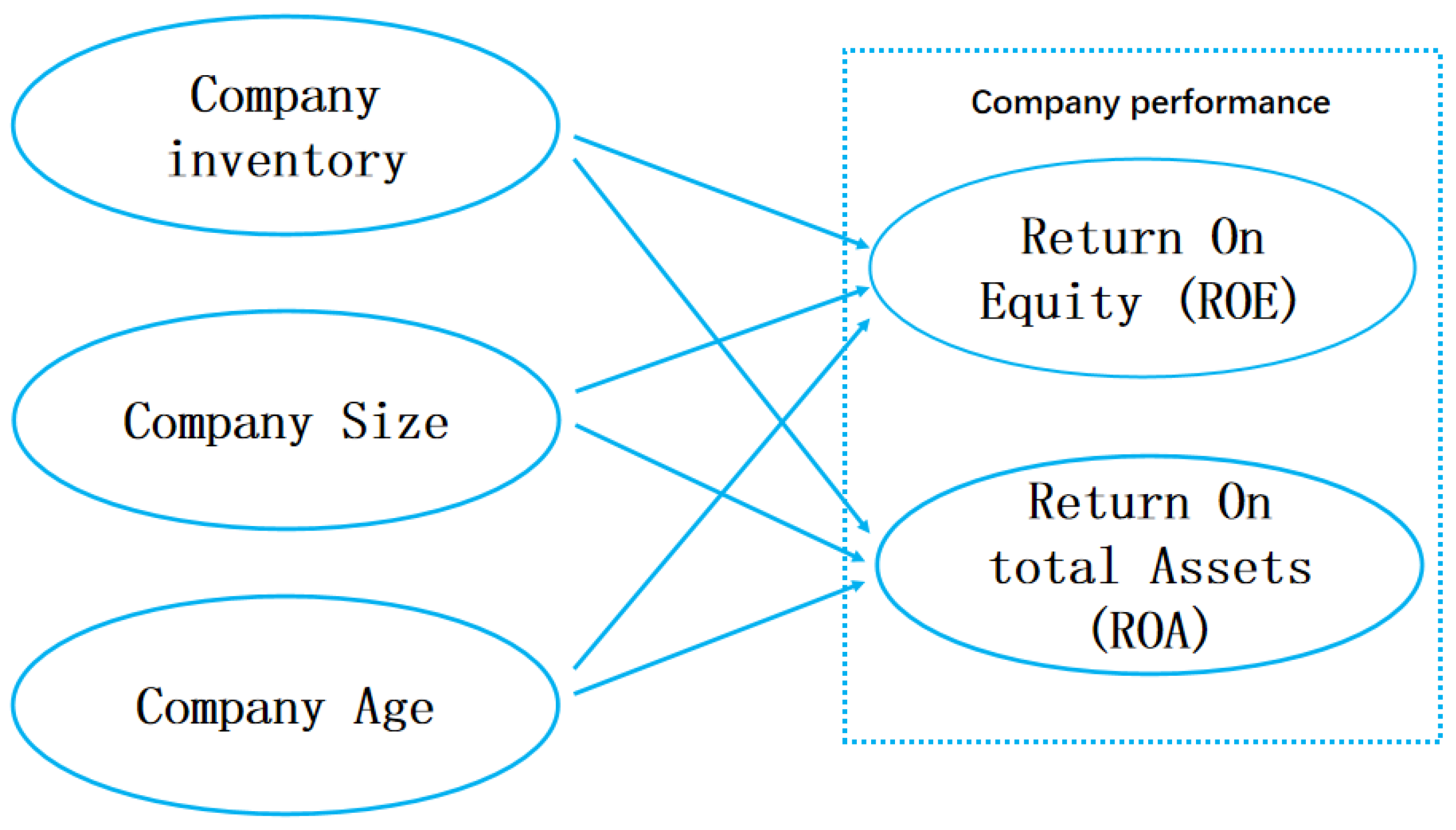
3.1. Theoretical Framework Model and Data Sources

Measurement of the Dependent Variable: Business performance is measured using Return on Assets (ROA) and Return on Equity (ROE). ROA and ROE are used as dependent variables to ensure the robustness of empirical results through mutual references. The calculation formulas are as follows: Return on Assets (ROA) = Earnings Before Interest and Taxes (EBIT)/Average Total Assets; Return on Equity (ROE) = Net Profit/Average Shareholders’ Equity.

Measurement of the Independent Variable [23]: Inventory Turnover (IT) is commonly used as a standard measure for inventory management in businesses. In this study, Inventory Turnover is used as a proxy variable to gauge the level of inventory management. The calculation formula is Inventory Turnover = Cost of Goods Sold (COGS)/Average Inventory, where Average Inventory = (Beginning Inventory + Ending Inventory)/2.

Selection of Control Variables: As identified in the Xiang et al. [2], company size (S) and company age (A) have been recognized as control variables in inventory models.

Here, we primarily study the relationship between inventory management level models and corporate performance, using inventory turnover ratio to represent inventory management level. This study also incorporates these variables into the model. Implementing inventory management allows businesses to eliminate waste, reduce inventory levels, and enable faster turnover of products and capital, thereby enhancing their competitive advantage in the market and maximizing profits. However, the implementation of inventory management requires businesses to invest more resources. For instance, implementing just-in-time procurement can significantly increase the costs associated with stock-outs. Since businesses aim to maximize overall effectiveness, there exists an optimal point for inventory management levels. Refs. [21,22] and others have identified a reversed U-shaped relationship between lean inventory management and corporate performance, the static model of inventory management is shown in Figure 1. Therefore, this section proposes the following hypothesis:

H: There is a reversed U-shaped relationship between inventory management levels and corporate performance.

China, as one of the largest manufacturing countries in the world and the country with the most comprehensive manufacturing sector, has also employed the following data types in previous inventory management research [2,25]. This paper conducts an empirical study using data from publicly listed manufacturing companies in China from 2019 to 2023. This section focuses on examining the impact of inventory management levels on corporate performance. Inventory management is a crucial aspect of corporate management, particularly for manufacturing enterprises. Therefore, this study selects listed manufacturing companies as its research subjects. To carry out the empirical research, this study excluded samples with missing or anomalous data, ultimately obtaining 11,160 unbalanced panel data points from 2232 companies across 30 manufacturing industries. The data for this study were sourced from the CSMAR (China Stock Market and Accounting Research) database.

3.2. Preliminary Analysis of Model Variables

Descriptive statistics were used to analyze the mean, minimum and maximum values, central tendency, and dispersion of all variables, as shown in

Table 1. Statistical analysis results of the related variables.

Variable	Mean	Std	Max	Min
Return on Assets (ROA)	3.3653	8.3166	78.5865	−216.0298
Return on Equity (ROE)	3.3602	28.8872	232.3628	1115.4
Inventory Turnover (IT)	4.428	4.0441	53.8295	0.0305
Company Size (S)	22.2971	1.2173	27.6400	17.9500
Company Age (A)	21.6039	5.7632	67	4

.

From Table 1, we observe that in terms of corporate performance among listed manufacturing companies in China, the mean Return on Equity (ROE) is 3.3602%, with a minimum value of −1115.4% and a maximum value of 288.8872%. The range of these values is quite large, and the standard deviation is 28.8872, indicating significant overall volatility. The mean Return on Assets (ROA) is 3.37653%, with a minimum value of −216.0928% and a maximum value of 78.5865%, as well as a standard deviation of 8.3166, showing relatively less fluctuation compared to ROE. This suggests that the overall performance level of listed manufacturing companies in China is relatively average, with considerable variability among companies. The mean Inventory Turnover (IT) ratio is 4.428, with a minimum value of 0.0305 and a maximum value of 53.8295, and a standard deviation of 4.0441. Compared to ROE and ROA, the Inventory Turnover ratio shows a larger range of fluctuation, indicating preliminary evidence of disparities in inventory management across different companies.

The mean company size (S) is 22.297, with a standard deviation of 1.2173, indicating that the overall scale of the manufacturing industry in China is quite large, with small differences among companies. The maximum age of companies (A) is 67 years, with a mean of 21.6039 and a standard deviation of 5.7632. This suggests that manufacturing companies in China have been established for a relatively long time, but there is also significant variation in their ages.

Additionally, we calculated the correlations between variables, as shown in

Table 2. Results of correlation analysis.

Variable	ROA	ROE	IT	S	A
ROA	1
ROE	0.6849 ***	1
IT	0.030	0.0116 *	1
S	0.1270 ***	−0.1193 ***	0.1273 ***	1
A	−0.0457 ***	−0.0186 **	0.0758 ***	0.1464 ***	1

. In the table, *** indicates $p<0.01$, ** indicates $p<0.05$, and * indicates $p<0.10$. It can be observed that the significant relationships are generally strong, but the correlations do not reach or approach 1. This indicates that the selected variables are not collinear, which meets the basic requirements.

3.3. Static Mathematical Model and Regression Analysis

In order to investigate the nonlinear influence of lean inventory on Return on Assets ($ROA$) and Return on Equity ($ROE$), this chapter sets the measurement model as follows.

$$\begin{array}{c}\hfill ROA=\alpha +{\alpha }_{1}IT+{\alpha }_2{IT}^2+{\alpha }_{3}S+{\alpha }_{4}A+e_1\\ \hfill ROE=\beta +{\beta }_{1}IT+{\beta }_2{IT}^2+{\beta }_{3}S+{\beta }_{4}A+e_2\end{array}$$

(1)

where $\alpha$, ${\alpha }_1$, ${\alpha }_2$, ${\alpha }_3$, ${\alpha }_4$, $\beta$, ${\beta }_1$, ${\beta }_2$, ${\beta }_3$ and ${\beta }_4$ are the coefficients of the model. $IT$ is the Inventory Turnover ratio. The Inventory Turnover ratio can represent the level of inventory management. S is the company size, and A is the company age, while $e_1$ and $e_2$ are the error terms.

Using the ‘regress’ function in MATLAB for linear regression, the following system parameters were obtained: $\alpha =-15.3505$, ${\alpha }_1=0.0452$, ${\alpha }_2=-0.0029$, ${\alpha }_3=0.9259$, and ${\alpha }_4=-0.0937$. The $R^2$ value was found to be 0.0207, which meets the basic requirements. The negative coefficient of $I{T}^2$ indicates that the quadratic function opens downward, which confirms a reversed U-shaped relationship. From the above, it can be seen that the hypothesis is valid: there is a U-shaped relationship between corporate performance and inventory management levels.

4. Dynamics Model of Inventory Management

The above model reflects the nonlinear characteristics between inventory and business performance. However, we obtained data for one year from the CSMAR database, and such data cannot capture the real-time dynamic adjustments of inventory. In today’s era of big data, it is essential to understand the real-time changes in inventory. Therefore, constructing a simple dynamic inventory management model is necessary. Studying the nonlinear changes in this dynamic model can provide a basis for safety stock prediction. The nonlinear discrete inventory management dynamics model is outlined in [2,7,8,9,10]. According to the sales resources $x_{n+1}$ for stage $n+1$, it is equal to the initial of the company plus the amount of inventory capital transferred to the sales portion at stage n (i.e., the sum of the inventory capital at stage n and the product of the inventory capital transfer rate $p{z}_n$). This means that $x_{n+1}$ is only related to the inventory resources and not to $x_n$. Therefore, we can determine $x_{n+1}$ in advance, which requires reconsidering the inventory management dynamics model to solve for $x_{n+1}$ ahead of time. The dynamic model of inventory management is revised as follows [10]:

$$\begin{array}{cc}\hfill & x_{n+1}=s+p·z_n\hfill \\ \hfill & y_{n+1}=q·x_{n+1}+r·y_n·z_n\hfill \\ \hfill & z_{n+1}=1-x_{n+1}-y_i+z_i.\hfill \end{array}$$

(2)

From Equation (2), the system changed from a three-dimensional system to a two-dimensional system.

$$\begin{array}{cc}\hfill & y_{n+1}=q·(s+p·z_n)+r·y_n·z_n\hfill \\ \hfill & z_{n+1}=1-s-p·z_n-y_n+z_n.\hfill \end{array}$$

(3)

Let $q=0.05$, $s=0.58$, and $r=0.72$ in Equation (4). This study uses MATLAB2019a software to write a program to solve Equation (4) and obtain the trajectory phase of the fractional-order inventory management system model, as shown in Figure 2. It can be seen from the trajectory phase diagram that the system is a periodic trajectory.

5. Dynamics Analysis

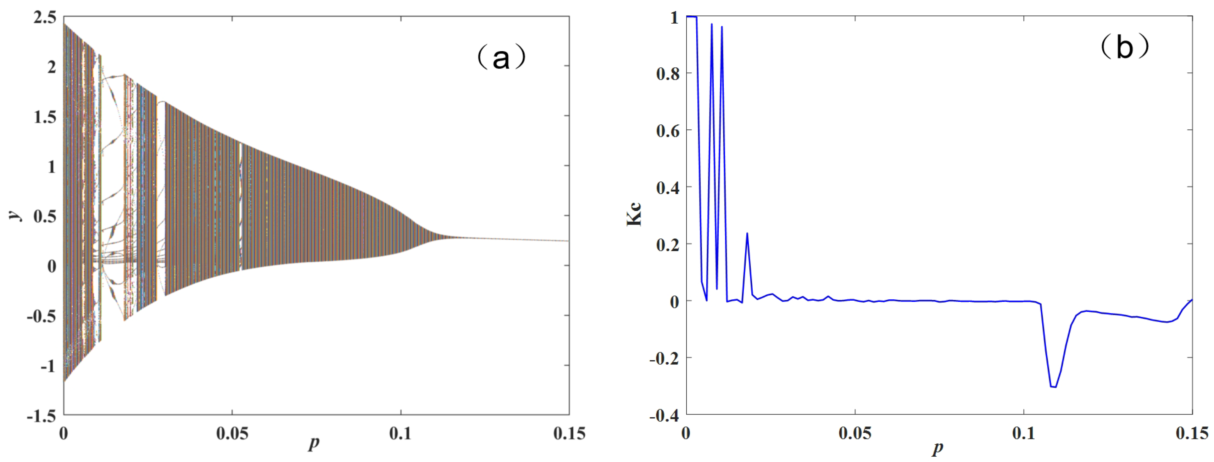
5.1. 0-1 Test and Bifurcation

The 0-1 test is a tool to analyze time series. Because the chaotic system is a series, it can also be used to analyze chaotic characteristics, and whether it is chaotic characteristics can be judged by whether the output result is 1.

Of course, there is also a visualization method, that is, the $p-q$ diagram is used to judge whether it is chaotic or not, and if the $p-q$ phase diagram shows Brownian motion, it is chaotic [25].

$$p_c\left(n\right)=\sum _{j=1}^n\varphi \left(j\right)cosjc$$

(4)

$$q_c\left(n\right)=\sum _{j=1}^n\varphi \left(j\right)sinjc$$

(5)

Here, $n=1,2,\dots ,n$. We can draw the trajectory diagram with $p_c$ and $q_c$ as the horizontal axis and vertical axis, respectively, and we can draw the $p-q$ phase diagram of $z_i$ with Matlab software, as shown in Figure 3.

In order to analyze the diffusion behavior of $p_c$ and $q_c$, we can calculate the displacement mean square deviation (MSD), with calculation formula being [26]

$$M_c\left(n\right)={\displaystyle \frac{1}{N}}\sum _{j=1}^N\left({\left[p_c(j+n)-p_c\left(j\right)\right]}^2+{\left[q_c(j+n)-q_c\left(j\right)\right]}^2\right).$$

(6)

where $n=N/10$; however, the total length N can be the length of the original sequence. Calculate $M_c\left(n\right)$ and then obtain the measure index $K_c$ of the 0-1 test.

$$K_c=\underset{n\to \infty }{lim}{\displaystyle \frac{log{M}_c\left(n\right)}{logn}}$$

(7)

Based on Equation (8), use MATLAB to calculate $K_c$ for the y sequence in the model. Calculate the $K_c$ value for System (2): When $p=0.01$, the 0-1 test $K_c$ result for the system is −0.0012, which is close to 0, indicating that the system exhibits periodic characteristics [25]. When $p=0.005$, the 0-1 test $K_c$ result for the system is 0.9963, which is close to 1, indicating that the system exhibits chaotic characteristics.

The bifurcation diagram is an important tool for characterizing dynamical systems. In continuous systems, bifurcation diagrams are drawn using the maximum value method of state variables. Since the values in continuous systems are continuous, whereas in discrete systems the values are finite, we can directly plot the corresponding variable values on the Y-axis [27].

By varying the parameter q while keeping other parameters constant, the bifurcation diagram and $K_c$ values of the inventory management system are illustrated as shown in Figure 4. From the diagram, it can be observed that at relatively small p values, the system exhibits intersections of chaotic and periodic behavior. As the p value increases, the system enters a periodic state, with corresponding $K_c$ values being around 0. The bifurcation diagram also shows that the system stabilizes through a gradual reduction in amplitude, indicating that the p value should neither be too large nor too small but should be within an appropriate range. When p is within [0, 0.006] [0.010, 0.012] [0.018, 0.019], the system is in a chaos state, with $K_c$ being equal to 1; in other regions, the system also remains in a periodic state.

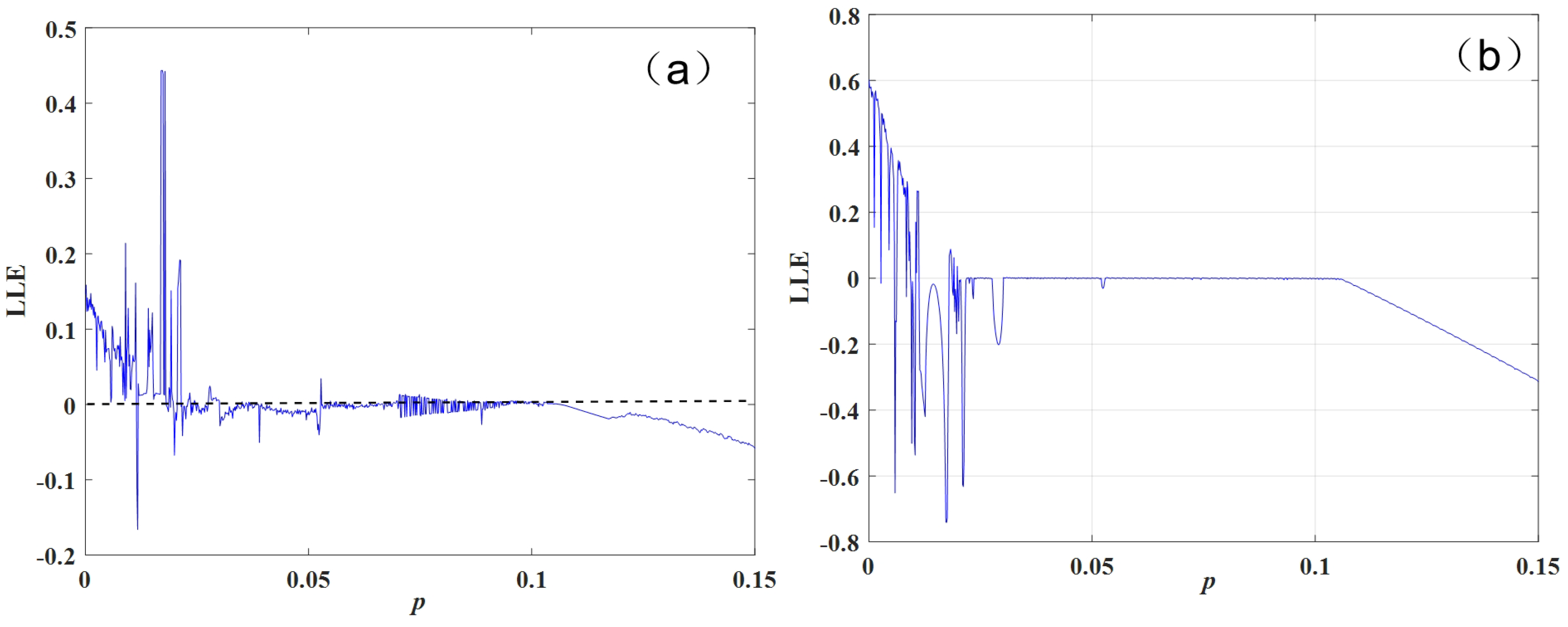
5.2. Largest Lyapunov Exponent (LLE)

In nonlinear systems, the fundamental characteristic of chaos is that motion is extremely sensitive to initial conditions [14]. A quantitative method that describes how trajectories starting from nearby initial conditions diverge exponentially over time is the Lyapunov exponent (LE). The Lyapunov exponent is a crucial quantitative indicator for assessing the dynamical properties of a system. It measures the average exponential rate of divergence or convergence between neighboring trajectories in phase space. If the Lyapunov exponent is greater than 0, it indicates a chaotic state; if it is less than or equal to 0, the system is in a periodic state [27,28].

Several methods are commonly used to compute the Lyapunov exponent, including the definition method, the Wolf method, the orthogonal method, and the small dataset method. Each of these methods has its advantages. This study employs two methods, the orthogonal method and the small dataset method, to verify the system’s dynamical behavior.

Orthogonal Method [28]: This method uses the Gram–Schmidt Renormalization (GSR) technique to track the behavior of divergent axes, allowing for the calculation of all Lyapunov exponents of a chaotic attractor. Detailed descriptions of this method can be found in reference [29] and will not be elaborated further here.

The specific steps for the small dataset method are as follows [30,31]:

S1: Reconstruction of phase space $\left\{Y_i\mid j=1,2,\cdots ,M\right\}$, from m and $\tau$. Find the nearest neighbor $Y_j^{\prime }$ of each point $Y_j$ in the phase space and limit the short score. That is,

$$d_j\left(0\right)=min∥Y_j-Y_j^{\prime }∥,\left|j-j^{\prime }\right|>P,$$

(8)

P is the average period of time series.

S2: For each point $Y_j$ in the phase space, the distance $d_j\left(i\right)$ after i discrete time steps of the adjacent point is calculated as follows:

$$d_j\left(i\right)=min∥Y_{j+i}-Y_{j+i}^{\prime }∥,i=1,2,\cdots ,min\left(M-j,M-j^{\prime }\right)$$

(9)

For each i, find the $lndj\left(i\right)$ average $y\left(i\right)$ of all j:

$$y\left(i\right)={\displaystyle \frac{1}{q\Delta t}}\sum _{j=1}^{q}ln{d}_j\left(i\right)$$

(10)

where q is the number of non-zero $d_j\left(i\right)$, with the regression line being made by the least square method, and the slope of the line is LLE.

Changing the system parameter p in the range [0, 0.15], while keeping other parameters of the inventory management system unchanged, we performed simulations using MATLAB to compare two algorithms. The largest Lyapunov exponent (LLE) system plots were generated using the ‘plot’ function, with the results being shown in Figure 5.

From the figure, the following can be observed in Figure 5a: The LLE values obtained using the small dataset method are relatively small compared to those obtained using the orthogonal method in Figure 5b.Additionally, the LLE values in Figure 5a are less accurate, particularly when the system’s numerical solution exhibits jumps. The LLE values show significant variation, which does not match the complexity of the actual system. Figure 5b show that the LLE values obtained using the orthogonal method are correct and more consistent.

When using MATLAB for computations, the simulation results in Figure 5a are faster than those in Figure 5b, indicating that the small dataset method is simpler and quicker to compute. The model’s behavior aligns closely with the actual inventory levels because, in reality, the resource transfer rate p varies, making it impossible for the inventory levels to continuously remain in a chaotic, periodic, or steady state.

Currently, we can only obtain annual data for various types of business data, and daily data cannot be precisely acquired, resulting in a relatively small dataset. Therefore, this paper simulates the relevant data. As shown in the figure above, the two graphs are largely consistent, indicating that the calculation of the system’s maximum Lyapunov exponent using a small dataset is reliable and applicable to real business data.

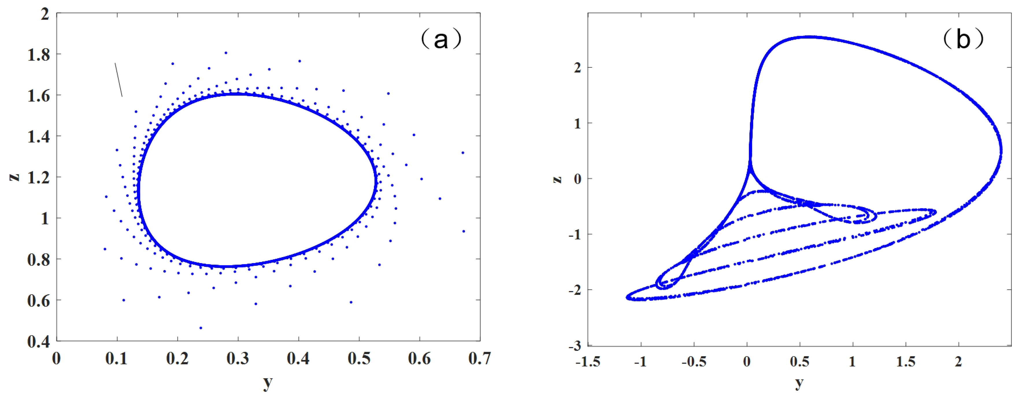
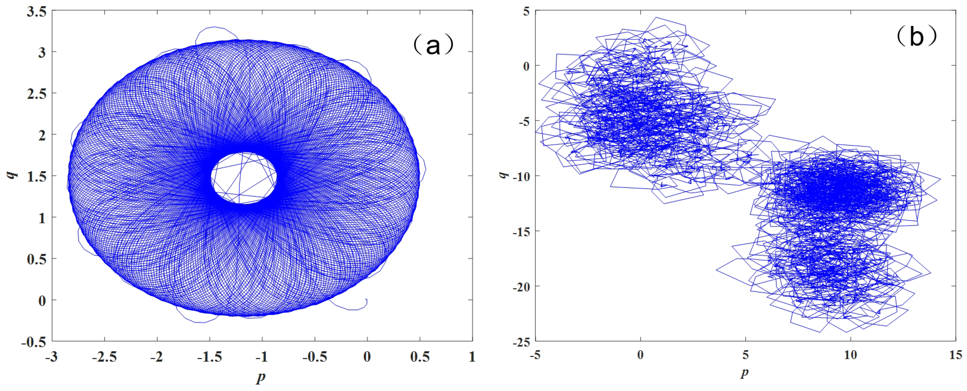
5.3. System Eigenvalue Trajectory Plot

System Eigenvalue Trajectory Plot is a graphical representation that shows the movement of eigenvalues in the complex plane as system parameters change [32]. It is useful for analyzing the stability and dynamics of a system. Complex the real part of the eigenvalues on the x-axis and the imaginary part on the y-axis. Change the system parameters, and compute and plot the corresponding eigenvalues to track their movement in the complex plane. Figure 6 shows the trajectory of the system eigenvalue with the change of parameter p.

Using system eigenvalue trajectories, a set of conjugate eigenvalues are highlighted in the plot, marked in red and green. Eigenvalues within the unit circle represent stable characteristics and align on a single line, indicating that the system is at a stable equilibrium point. The equilibrium points alternate between being inside and outside the unit circle. When the parameter p is relatively small, the system exhibits alternating chaotic and periodic behavior. When the eigenvalues are within the unit circle and lie on the line where the imaginary part is zero, this also reflects the system’s stability.

The trajectory plot of the system’s eigenvalues shows that if the system’s inventory changes periodically, it remains stable and controllable. In this case, the system’s eigenvalues are within the unit circle.

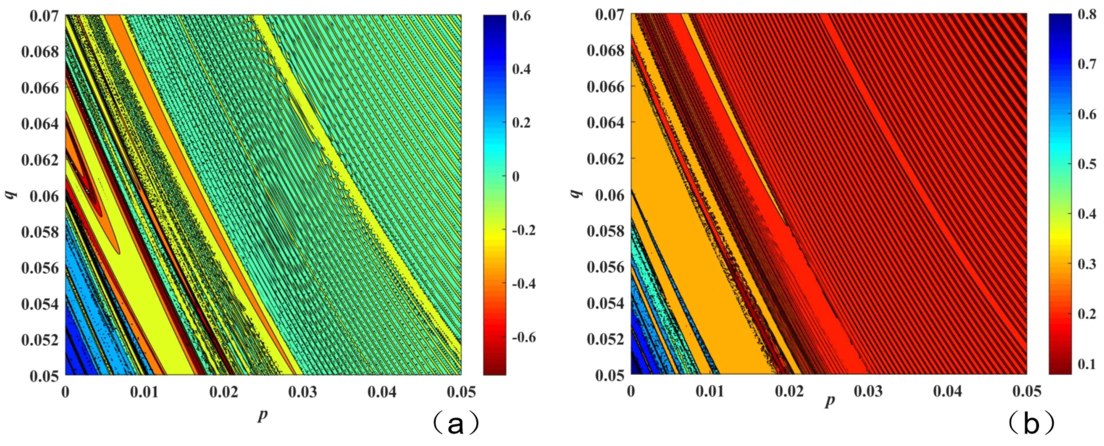
5.4. Two-Parameter Variation

We describe the dynamical characteristics of a system under two-parameter variation using the LLE and complexity [17] with two-parameter variations. Complexity is usually referred to as the complexity of the information, represented by SE and C0, respectively. This paper uses SE complexity for description, with the relevant mathematical formulas being provided in the literature [17] and not repeated here. The maximum Lyapunov exponent and SE complexity under variations in parameters p ∈ [0.05, 0.07] and q ∈ [0, 0.05] were obtained through Matlab simulations, as shown in Figure 7. Matlab source code for the largest Lyapunov exponent under two-parameter variation is provided in Appendix A.

In Figure 7a,b, different colors represent different values (with the color sequence from low to high being black, red, orange, yellow, green, cyan, and blue). By analyzing the two figures, it can be observed that they are generally consistent, indicating that the system complexity and the maximum Lyapunov exponent describe the system’s dynamical behavior in a similar manner. Additionally, it is evident that when p is relatively small, the system exhibits high complexity. Once p exceeds 0.01, the system complexity remains relatively low, between 0.2 and 0.3, indicating that the system is either periodic or in a stable state. By examining the color maps of the system under variations of the two parameters, we can choose an appropriate parameter range for the system.

6. Conclusions

Firstly, using a sample of listed manufacturing companies in China, a static inventory model was constructed to empirically test the impact of inventory management on performance. The conclusions are as follows:

Nonlinear Relationship: Data from CSMAR have demonstrated that our hypothesis of an inverted U-shaped relationship between inventory management and company performance is correct. The inverted U-shape indicates that the system has a maximum point, suggesting that there is an optimal level of lean inventory management. Implementing inventory management to a moderate extent can significantly improve performance.

Dynamic Model Analysis: Using dynamic models, this study explored how inventory transfer rates affect inventory levels through 0-1 tests, bifurcation diagrams, and the maximum Lyapunov exponent. It was found that suitable parameter values are necessary; constant and oscillatory inventory levels are not optimal.

Besesides, this study investigated only the nonlinearity of inventory management using data from the Chinese manufacturing sector. Future research could expand this analysis to other countries and other sectors, such as supermarkets, construction, and computer hardware.

References

1. Qian, Z.; Wang, C.X.; Yang, H. Association between corporate diversification strategies and inventory performance: A firm-level investigation. Int. J. Oper. Prod. Manag. 2024. [Google Scholar] [CrossRef]
2. Wan, X.; Britto, R.; Zhou, Z. In search of the negative relationship between product variety and inventory turnover. Int. J. Prod. Econ. 2020, 222, 107503. [Google Scholar] [CrossRef]
3. Halat, K.; Hafezalkotob, A. Modeling carbon regulation policies in inventory decisions of a multi-stage green supply chain: A game theory approach. Comput. Ind. Eng. 2019, 128, 807–830. [Google Scholar] [CrossRef]
4. Žic, J.; Žic, S.; Đukić, G.; Dabić-Miletić, S. Exploring Green Inventory Management through Periodic Review Inventory Systems—A Comprehensive Literature Review and Directions for Future Research. Sustainability 2024, 16, 5544. [Google Scholar] [CrossRef]
5. Qu, S.; Zhou, Y.; Ji, Y.; Dai, Z.; Wang, Z. Robust maximum expert consensus modeling with dynamic feedback mechanism under uncertain environments. J. Ind. Manag. Optim. 2024, 21, 524–552. [Google Scholar] [CrossRef]
6. Engebrethsen, E.; Dauzère-Pérès, S. Transportation mode selection in inventory models: A literature review. Eur. J. Oper. Res. 2019, 279, 1–25. [Google Scholar] [CrossRef]
7. Zhang, S.; Huang, K.; Yuan, Y. Spare Parts Inventory Management: A Literature Review. Sustainability 2021, 13, 2460. [Google Scholar] [CrossRef]
8. Vastag, G.; Whybark, D.C. Inventory management: Is there a knock-on effect? Int. J. Prod. Econ. 2005, 93–94, 129–138. [Google Scholar] [CrossRef]
9. Eroglu, C.; Hofer, C. Lean, leaner, too lean? Chopra The inventory performance link revisited. J. Oper. Manag. 2010, 29, 356–369. [Google Scholar] [CrossRef]
10. Burawat, P. The relationships among transformational leadership, sustainable leadership, lean manufacturing and sustainability performance in Thai SMEs manufacturing industry. Int. J. Qual. Reliab. Manag. 2019, 36, 1014–1036. [Google Scholar] [CrossRef]
11. Buisman, M.E.; Rohmer, S.U.K. Inventory dynamics at the retailer—An economic and environmental analysis of packaging fresh produce. Sustain. Anal. Model. 2023, 3, 100020. [Google Scholar] [CrossRef]
12. Yao, H.; Sheng, Z. An improved feedback control method in economic chaos model. J. Syst. Eng. 2002, 6, 507–511+518. [Google Scholar]
13. Chen, G.; Yao, H.; Sheng, Z. Synchronous control of chaotic system in inventory management. Forecast 2003, 22, 38–41+24. [Google Scholar]
14. Lei, T.; Li, R.Y.M.; Fu, H. Dynamics Analysis and Fractional-Order Approximate Entropy of Nonlinear Inventory Management Systems. Math. Probl. Eng. 2021, 2021, 5516703. [Google Scholar] [CrossRef]
15. Yuan, L.; Yang, X.; Zhong, R. Fractional-order approximate entropy algorithm. J. Xi’an Univ. Technol. 2020, 36, 575–580. [Google Scholar]
16. Lei, T.; Li, R.Y.M.; Jotikastira, N.; Fu, H.; Wang, C. Prediction for the Inventory Management Chaotic Complexity System Based on the Deep Neural Network Algorithm. Complexity 2023, 2023, 9369888. [Google Scholar] [CrossRef]
17. Lei, T.; Li, R.Y.M.; Deeprasert, J.; Fu, H. Dynamics and Complexity Analysis of Fractional-Order Inventory Management System Model. Fractal Fract. 2024, 8, 258. [Google Scholar] [CrossRef]
18. Yigit, F.; Easnaf, S. A new fuzzy C-means and AHP-based three phased approach foumultiple criteria ABC inventory classificatigon. J. Intell. Manuf. 2021, 32, 1517–1528. [Google Scholar] [CrossRef]
19. Perez, H.D.; Hubbs, C.D.; Li, C.; Grossmann, I.E. Algorithmic Approaches to Inventory Management Optimization. Processes 2021, 9, 102. [Google Scholar] [CrossRef]
20. Zhong, Z.; Yuan, M.; He, Z. Data-Driven Algorithms for Two-Location Inventory Systems. Systems 2024, 12, 153. [Google Scholar] [CrossRef]
21. Bendig, D.; Strese, S.; Brettel, M. The link between operational leanness and credit ratings. J. Oper. Manag. 2016, 52, 46–55. [Google Scholar] [CrossRef]
22. Chen, G.; Li, X. Research on the Impact Mechanism of Lean Inventory Management on Corporate Performance from an Innovation Perspective: The Mediating Effect of Management Innovation. Sci. Technol. Manag. Res. 2019, 39, 207–214. [Google Scholar]
23. Wang, C.; Zhang, J.; Ma, J. The Impact of Lean Inventory Management on Firm Performance—Empirical Evidence from Chinese Listed Manufacturing Firms. Manag. Rev. 2017, 29, 165. [Google Scholar]
24. Centobelli, P.; Cerchione, R.; Singh, R. The impact of leanness and innovativeness on environmental and financial performance: Insights from Indian SMEs. Int. J. Prod. Econ. 2019, 212, 111–124. [Google Scholar]
25. Gottwald, G.A.; Melbourne, I. The 0-1 test for chaos: Areview. In Chaos Detection and Predictability; Springer: Berlin/Heidelberg, Germany, 2016; pp. 221–247. [Google Scholar]
26. He, S.; Sun, K.; Peng, Y. Detecting chaos in fractional-order nonlinear systems using the smaller alignment index. Phys. Lett. A 2019, 383, 2267–2271. [Google Scholar] [CrossRef]
27. Li, Y.; Li, C.; Yu, W.; Lei, T.; Li, R.Y.M. Symmetric Pseudo-Multi-Scroll Attractor and Its Application in Mobile Robot Path Planning. Symmetry 2024, 16, 868. [Google Scholar] [CrossRef]
28. Lei, T.; He, J.; Wang, Y.; Zang, H.; Huang, L.; Fu, H. Analysis of fractional order nonlinear system based on Adomian decomposition method and realization of Lyapunov exponent algorithm. J. Vib. Shock. 2021, 40, 1–6. [Google Scholar]
29. Fu, H.; Lei, T. Adomian Decomposition, Dynamic Analysis and Circuit Implementation of a 5D Fractional-Order Hyperchaotic System. Symmetry 2022, 14, 484. [Google Scholar] [CrossRef]
30. Haiyan, F.; Tengfei, L.; Miaomiao, X.; Feng, C.; Minglei, J.; Tingyang, Y. Identification and Analysis of Tool Wear Signal in CNC Machine Tool Based on Chaos Method. In Proceedings of the 2021 IEEE International Conference on Prognostics and Health Management (ICPHM), Detroit (Romulus), MI, USA, 7–9 June 2021; pp. 1–5. [Google Scholar]
31. Luo, L.; Li, Y.; Li, T.; Dong, Q. Research and simulation of Lyapunov’s exponents. Comput. Simul. 2005, 22, 285–288. (In Chinese) [Google Scholar]
32. Li, Y.; Li, C.; Tang, Q.; Gao, Y.; Lei, T. Various Dynamics of Amplitude Regulation Within a Class of 3D Rulkov Neurons. In IEEE Transactions on Circuits and Systems I: Regular Papers; IEEE: New York, NY, USA, 2024. [Google Scholar] [CrossRef]
Figure 1. Static model of inventory management.
Information 15 00785 g001
Figure 2. Numerical two-dimensional inventory management system (3) trajectory diagram: (a) y z attractor with p = 0.1 ; (b) y z attractor with p = 0.05 .
Information 15 00785 g002
Figure 3. p q phase diagram. (a) p q phase diagram with p = 0.1 ; (b) p q phase diagram with p = 0.005 .
Information 15 00785 g003
Figure 4. Bifurcation diagram and K c ofthe inventory management system with parameter p variation: (a) bifurcation diagram of the system; (b) LLE of the system.
Information 15 00785 g004
Figure 5. LLE of inventory management system with parameter p variation: (a) orthogonal method; (b) small dataset method.
Information 15 00785 g005
Figure 6. Trajectory of the system eigenvalue.
Information 15 00785 g006
Figure 7. LLE and SE complexity of inventory management system with two-parameter p and q variation: (a) LLE; (b) SE complexity.
Information 15 00785 g007