3.4. Experimental Setup
To validate the proposed approach, an analysis was conducted using the NARX and LSTM models with Kalman smoothing for a first-order system. This system was applied to two hydrological stations with a first-order system by using six inputs and two outputs with off-line training. In this water level prediction model, three different Kalman smoothing techniques are employed to assess the robustness of the models in predicting water levels. A comparative visualization is provided, showing both the real and estimated signals from the nonlinear hybrid models, along with the graphical responses of the three Kalman smoothing techniques for each model. Additionally, a quantitative evaluation is performed using four machine learning regression metrics, as previously described, allowing for a thorough assessment of the model’s performance. The algorithms were implemented using MATLAB (R2023b). In order to perform the training and validation of the neural network, the MATLAB function PREPARETS is used, where the time steps are automatically divided into training, validation, and test sets. The training set is used to teach the network, and the training continues as long as the network continues improving on the validation set.
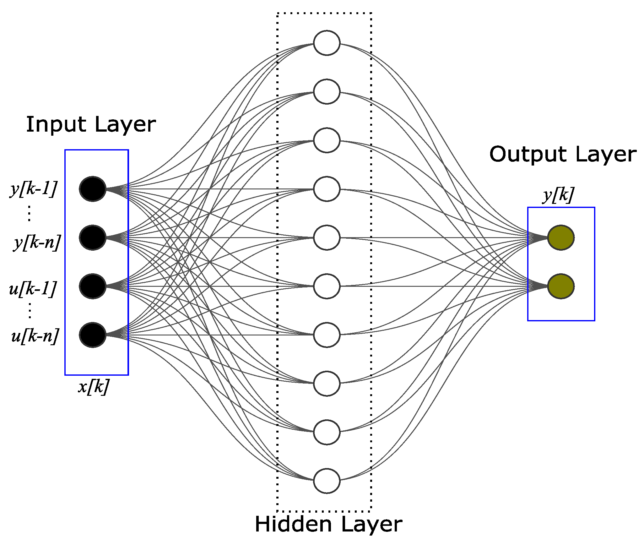
The feedforward network structure for the NARX neural network approach and the LSTM recurrent neural network includes a hidden layer with 10 nodes. The ReLU (rectified linear unit) activation function was selected for the NARX model since this piecewise linear function generates an output directly proportional to the input if it is positive or a value of zero otherwise.
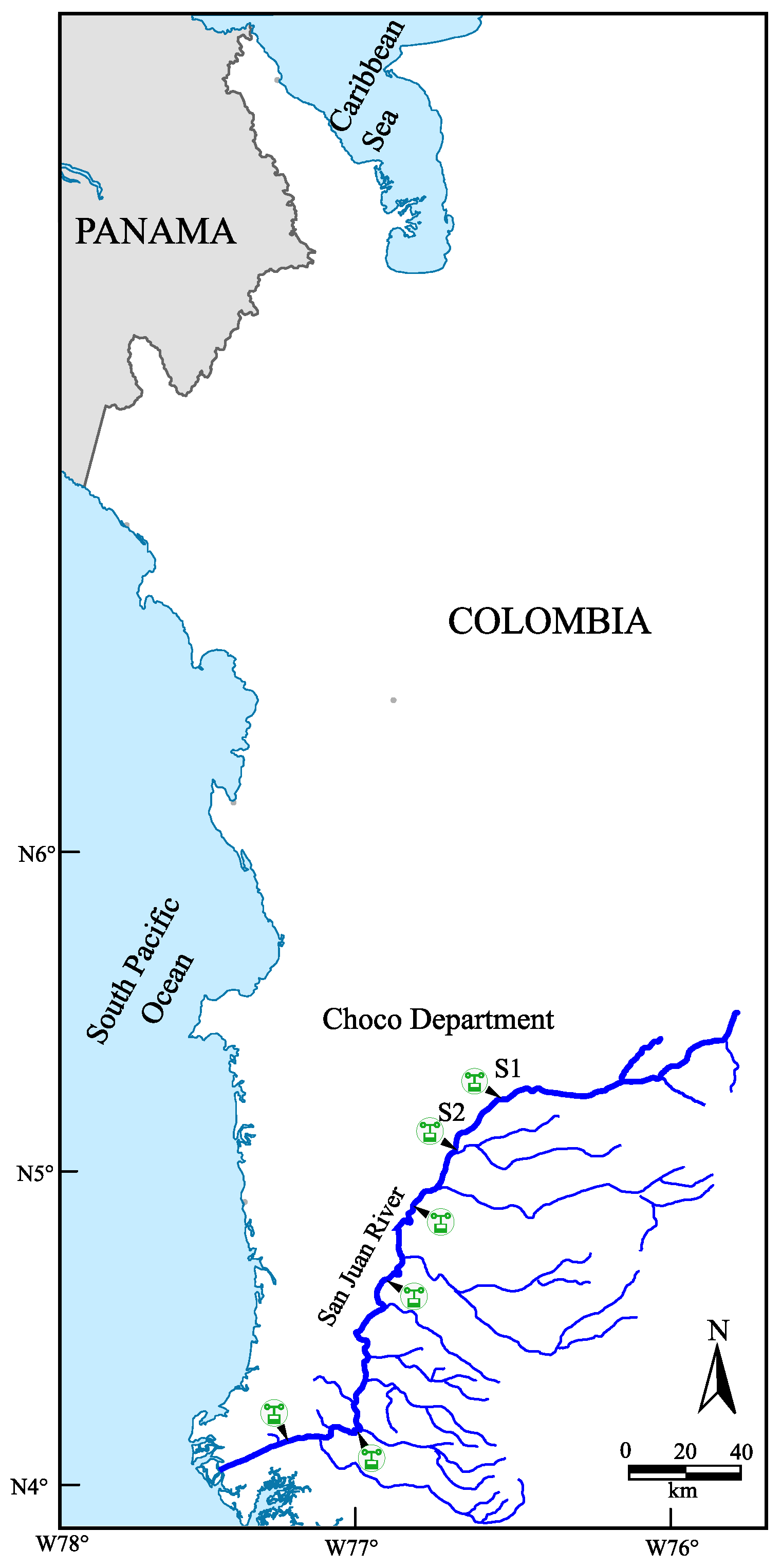
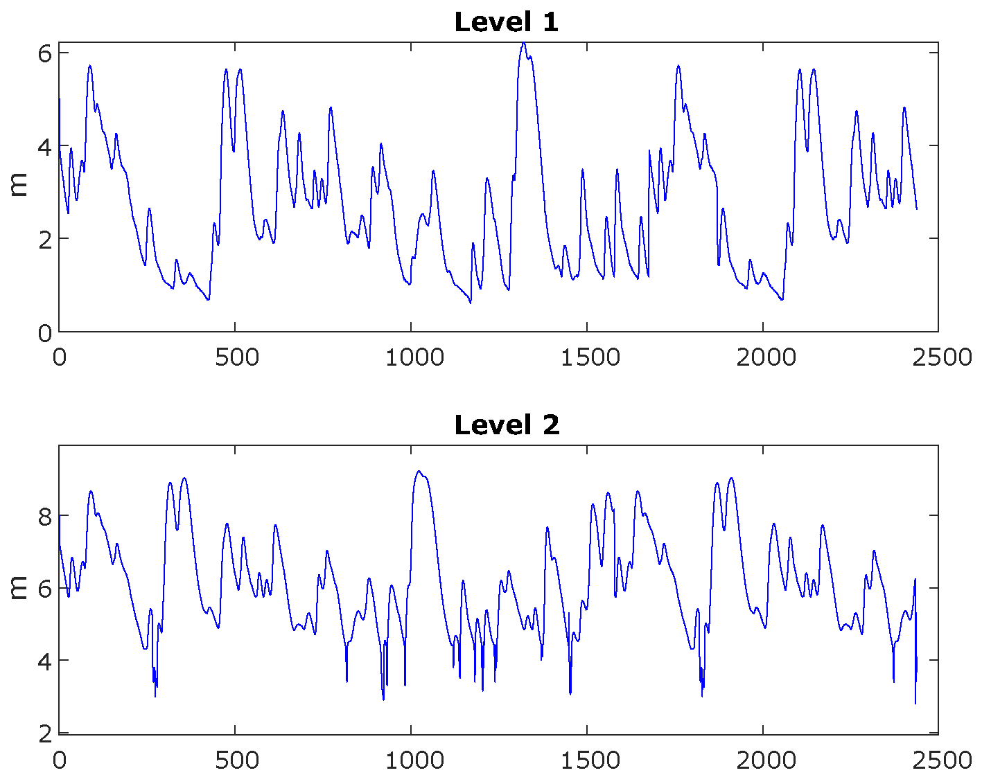
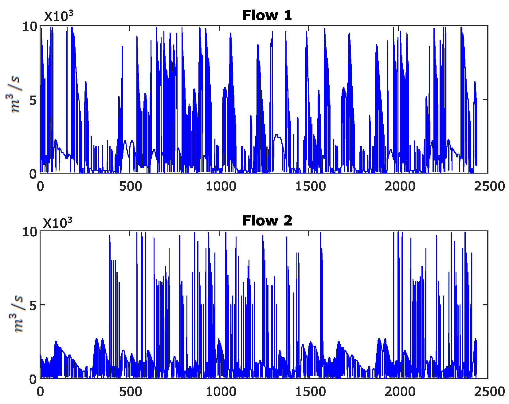
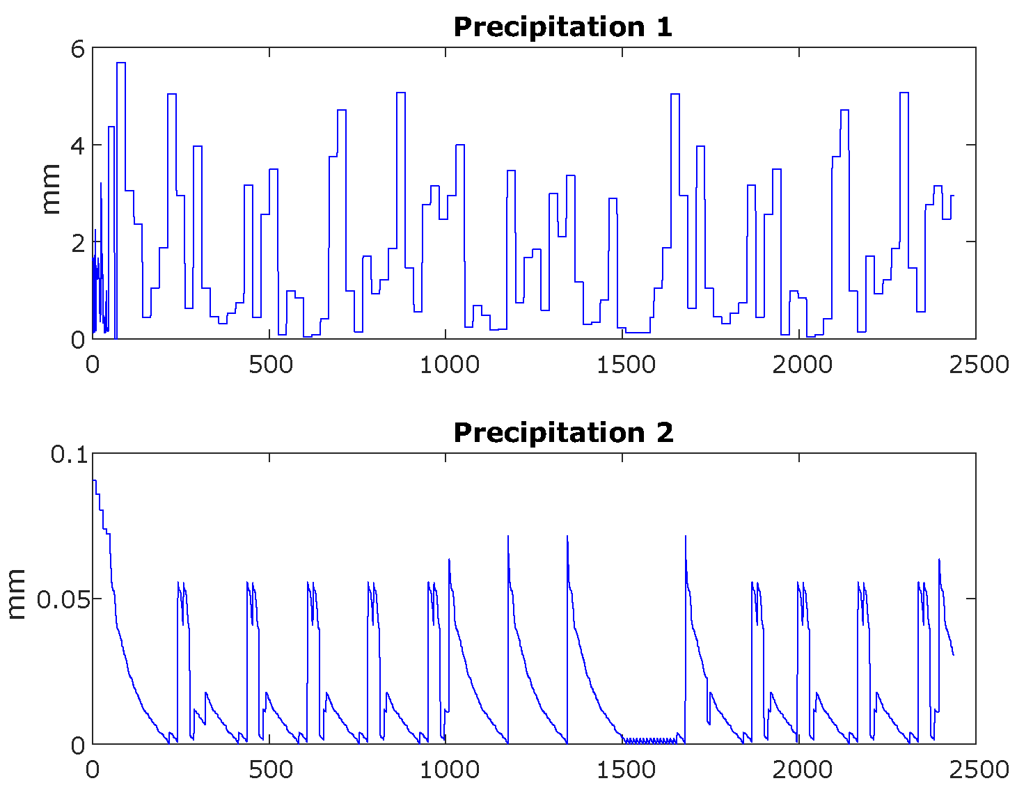
For this study, six activation functions in the input layer, one hidden layer with 10 nodes, and two outputs were considered. A feedforward network and an LSTM recurrent neural network were selected as the framework for the development of the hybrid NARX with Kalman smoothing and LSTM with Kalman smoothing models. Both models were trained off-line, using a dataset composed of 2438 samples corresponding to the three hydrological variables previously mentioned, measured at two hydrological stations located at the San Juan River in the department of Chocó, Colombia. It is worth noting that the real measurements in the dataset were not filtered before the training stage.
This approach allows for capturing the complex dynamics of the time series related to flow, water level, and precipitation. The hybrid models take advantage of the capacity of the smoothed Kalman filter to improve the accuracy of the predictions, integrating temporal information and correcting past estimates, which results in more robust and reliable predictions for flood risk management in the region.
The combined NARX and LSTM model, coupled with the smoothed Kalman filter, is essential for hydrological prediction, as it has the ability to handle external disturbances, such as white noise, which significantly improves the accuracy of the estimates. This approach is ideal for modeling complex phenomena such as river water levels, where environmental conditions and temporal variability play a key role in the evolution of the data. It is worth mentioning that exponential smoothing is configured by using the smoothing parameter of , and the Savitzky–Golay smoothing filter sets the number of convolution coefficients at .
3.7. LSTM Estimation Results with the Three Kalman Smoothing Techniques: Exponential Smoothing, Savitzky–Golay Smoothing, and Rauch–Tung–Striebel (RTS)
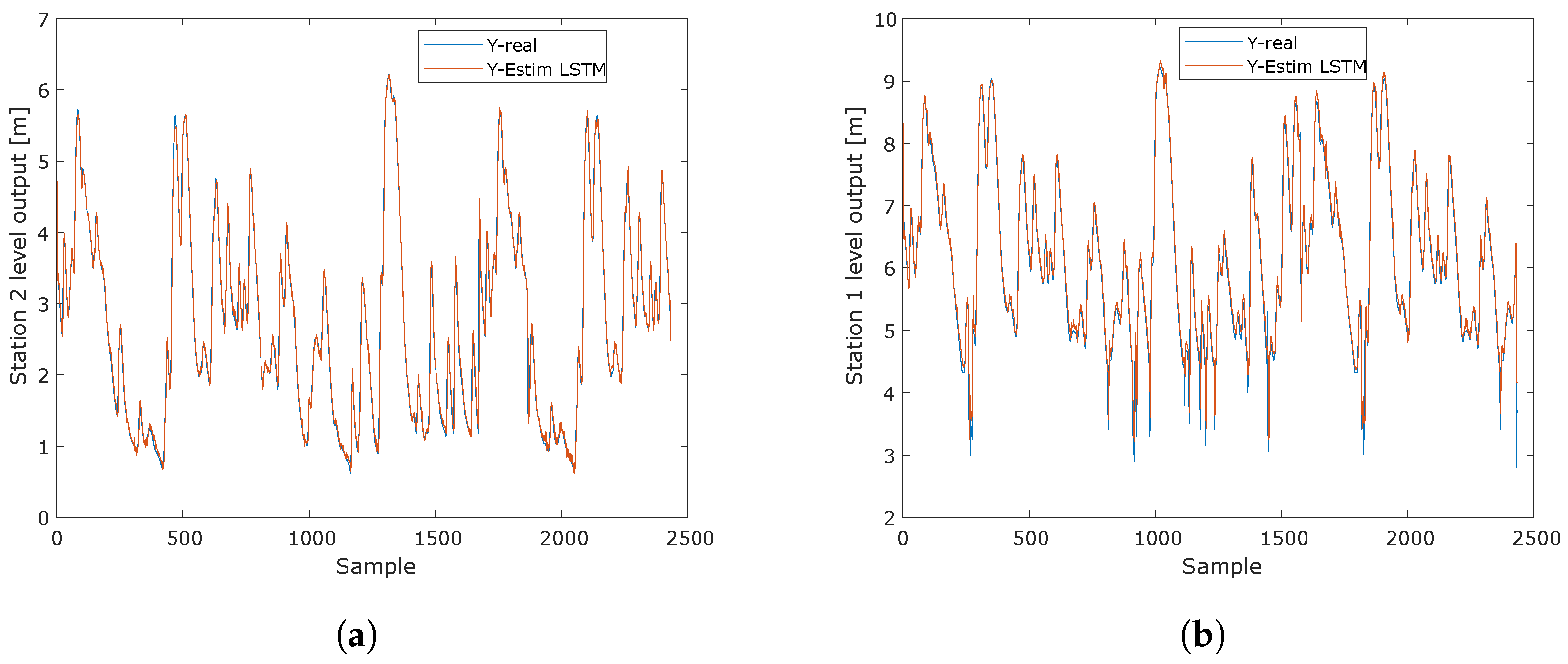
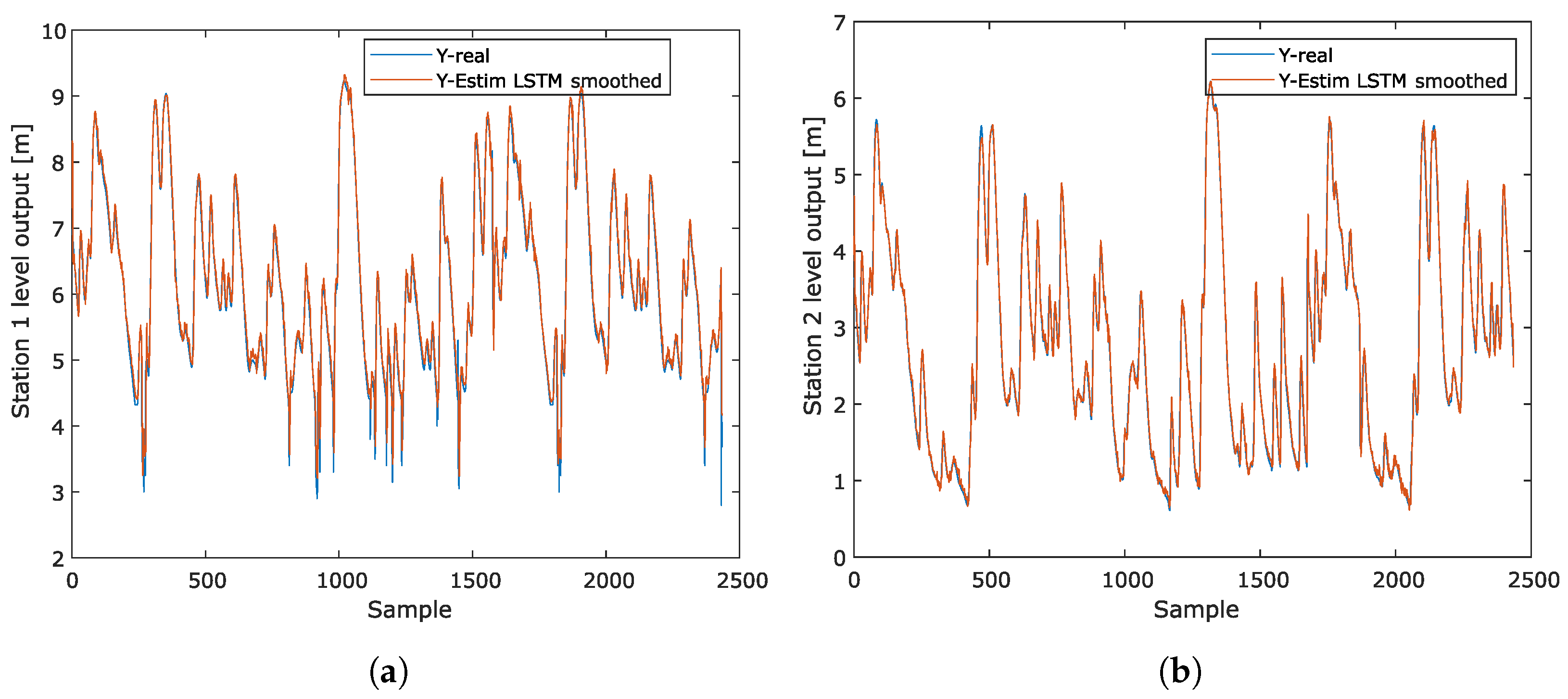
The results obtained for the LSTM model applied to both water level outflows can be seen in
Figure 12. Specifically,
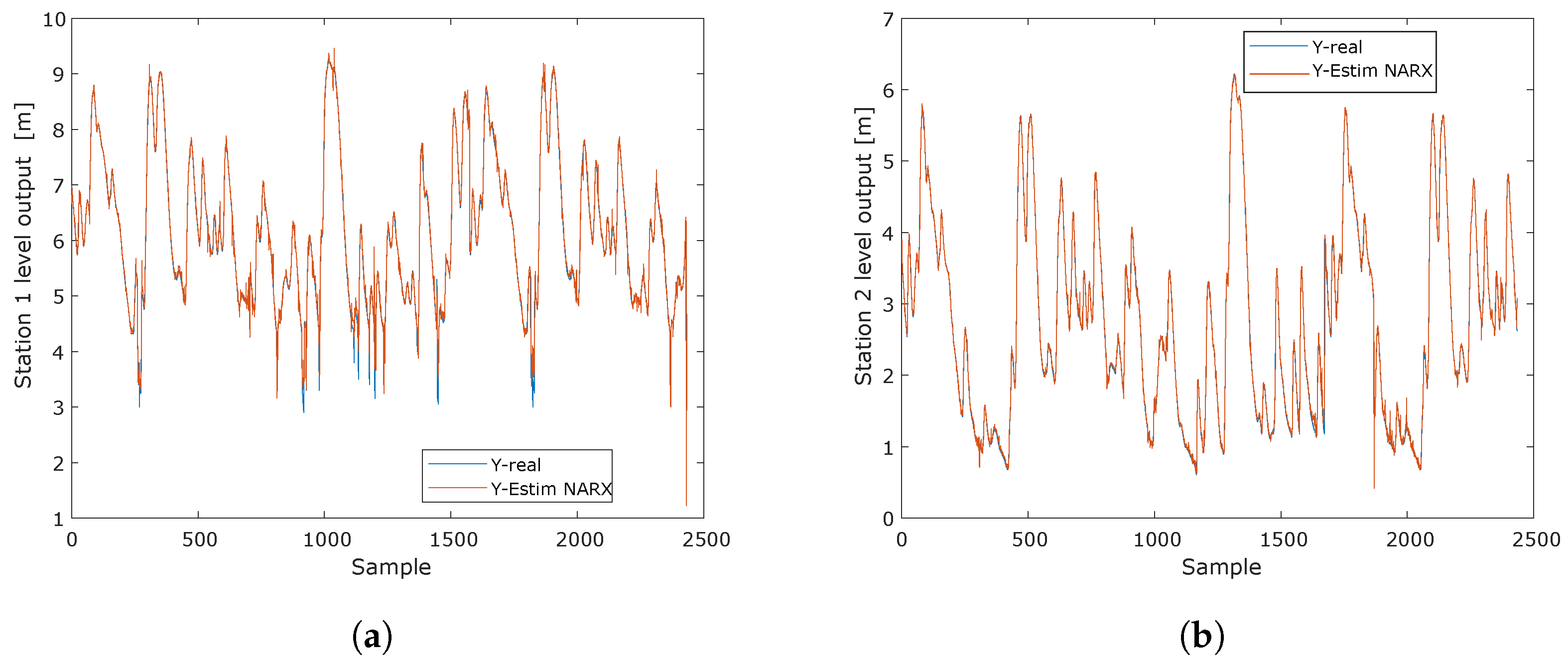
Figure 12a illustrates the short-term estimates for the first water level output, comparing the estimated signal with the actual measurements. Similarly,
Figure 12b presents the short-term prediction for the second water level output, together with the corresponding actual measurements, allowing for the accuracy of the model to be evaluated.
This type of comparative analysis allows for a clear visualization of the performance of the LSTM model and its ability to follow the evolution of water levels at both outlets.
The responses shown in
Figure 13 using the exponential smoothing method illustrate how the smoothed values fit a time series, helping to reduce noise and reveal the overall underlying trend in the data. This plot highlights the ability of smoothing to follow the general behavior of the data, eliminating short-term fluctuations. In
Figure 13a,b, the responses for the first and second water level outputs, respectively, using the exponential smoothing method are presented. The plots reflect how the method captures the main trends at both outlets, conforming to the overall patterns of water level behavior while mitigating the effects of noise.
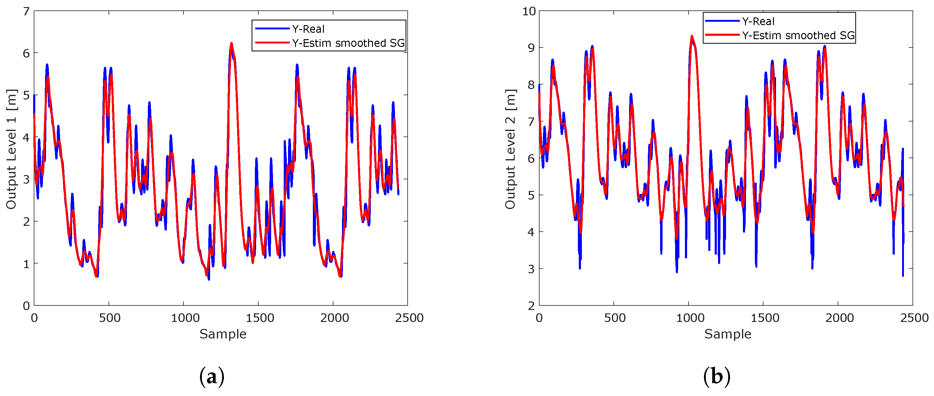
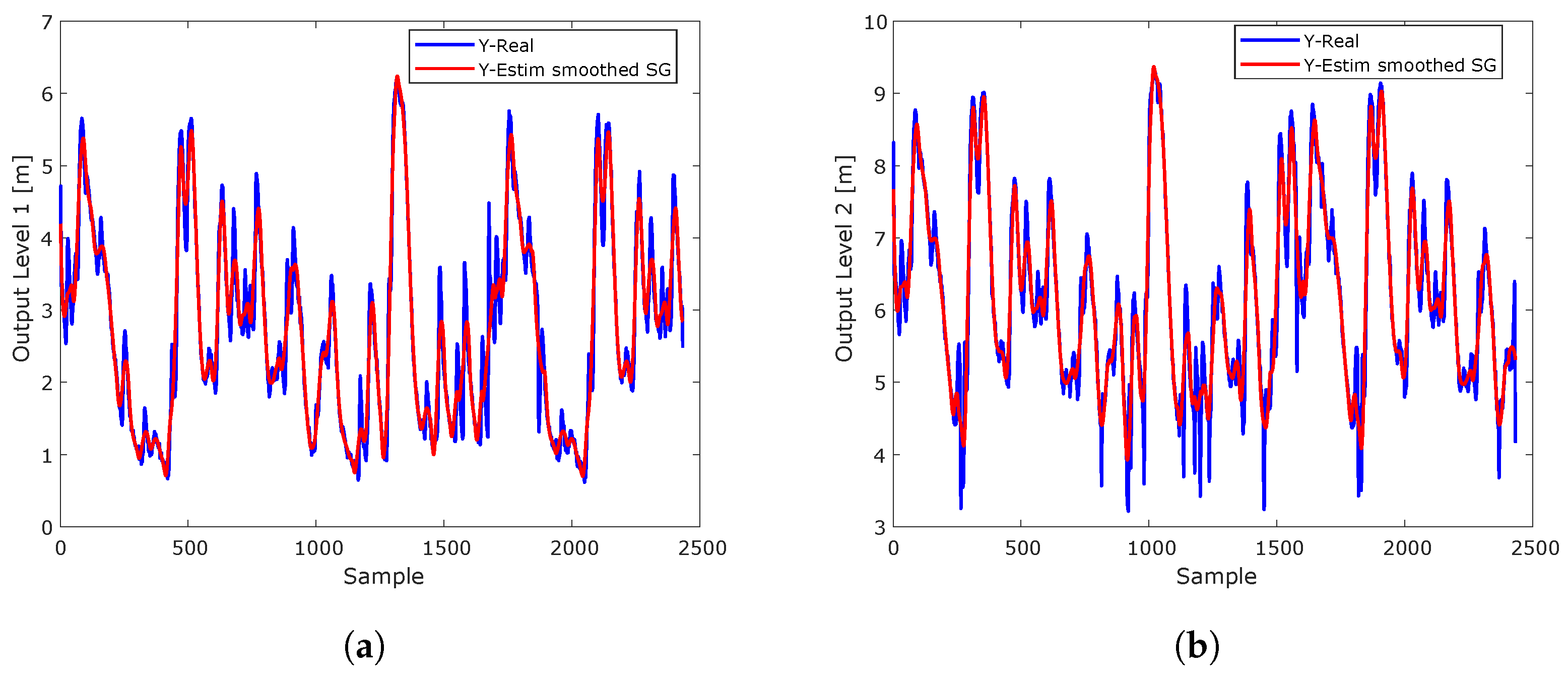
The Savitzky–Golay smoothing filter coupled to an LSTM network for two outputs, as presented in
Figure 14, illustrates how the method can reduce noise in the data and improve the accuracy of the LSTM model in predicting water level trends. This approach combines the filter’s ability to preserve relevant patterns with the ability of the LSTM to capture long-term dependencies in time series. In
Figure 14a, the first smoothed water level output is shown, and in
Figure 14b, the second output is shown, providing a more accurate and robust prediction of water levels.
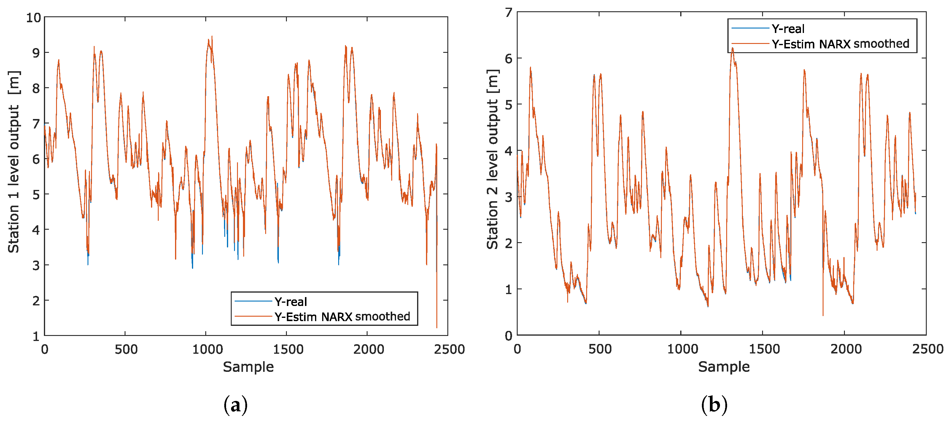
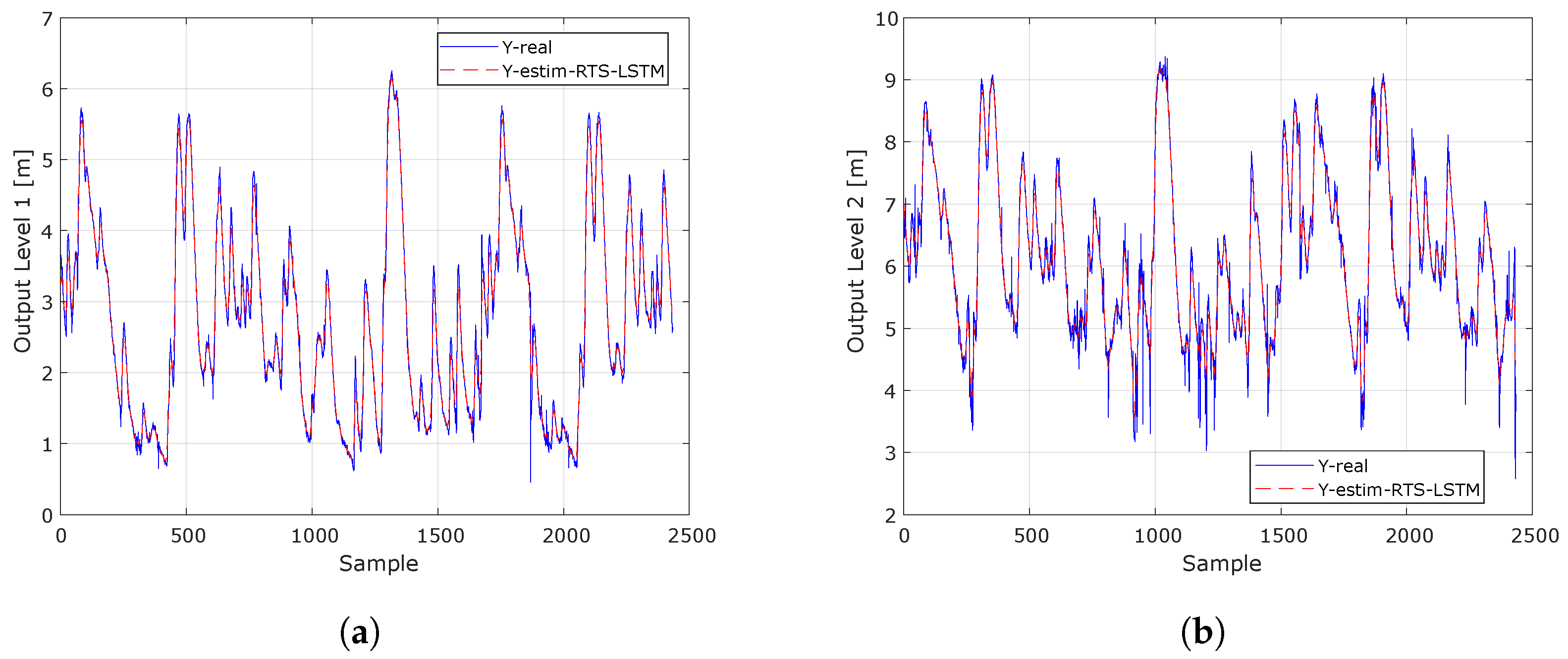
The smoothed Kalman filter using the Rauch–Tung–Striebel (RTS) algorithm applied to two water level outputs allows for observing how the model estimates align with actual measurements over time, facilitating the evaluation of its performance at each monitoring station.
Figure 15 illustrates the effectiveness of the filter in reducing noise, resulting in more consistent estimates that accurately reflect water level dynamics. A good fit between the curves of the actual outputs and the estimates indicates that the model is able to adequately capture variations and trends in the data, a crucial aspect for efficient water resource management. In addition, this graphical representation facilitates the detection of patterns and changes in water levels, which is particularly useful for forecasting floods and droughts.
Figure 15a shows the response for the first water level output, while
Figure 15b shows the response for the second output, using the smoothed Kalman filter with the Rauch–Tung–Striebel (RTS) algorithm.
Table 5 and
Table 6 present a quantitative analysis of the four regression metrics used in this research: MSE, KGE, NSE, and MAE. These metrics allow us to evaluate the accuracy of the estimates obtained using the NARX neural network model coupled with three Kalman smoothing techniques. This facilitates the evaluation of the model’s performance and its ability to generate accurate water level predictions.
In the results presented in both tables, the Narx-EXP model (NARX coupled with the exponential smoothing technique) shows the best performance in terms of accuracy and predictive ability for both Output 1 and Output 2. In Output 1, the MSE of Narx-EXP is the lowest (0.0013), with a KGE of 0.9968, an NSE of 0.9961, and an MAE of 0.0123, indicating exceptional performance in predicting water levels. In Output 2, Narx-EXP also outperforms the other models, with an MSE of 0.0078, a KGE of 0.9887, an NSE of 0.9812, and an MAE of 0.0308. This shows that exponential smoothing considerably improves prediction accuracy for both outputs, significantly reducing errors and increasing model efficiency compared to the base Narx model. In comparison, the base Narx model has a much higher MSE at both outputs (0.0062 for Output 1 and 0.0248 for Output 2), with lower KGE and NSE, showing its lower ability to predict water levels accurately.
On the other hand, the Savitzky–Golay (SG) and Rauch–Tung–Striebel (RTS) smoothing techniques also improve the performance of the Narx model, although not as markedly as exponential smoothing. Narx-SG, which uses Savitzky–Golay smoothing, has an MSE of 0.0432 for Output 1 and 0.0199 for Output 2, with the KGE and NSE lower than those of Narx-EXP but still better than those of the base model. The MAE of Narx-SG is also higher compared to Narx-EXP, reaching values of 0.0325 for Output 1 and 0.0623 for Output 2. Finally, Narx-RTS, which uses Rauch–Tung–Striebel smoothing, shows solid performance, especially for Output 1, with an MSE of 0.0135, a KGE of 0.9901, an NSE of 0.9921, and an MAE of 0.0463. For Output 2, its results are also quite good, with an MSE of 0.0123, a KGE of 0.9812, an NSE of 0.9766, and an MAE of 0.0548, placing it as the second best option after Narx-EXP. In summary, Narx-EXP offers the best accuracy and efficiency in water level prediction, while Narx-RTS and Narx-SG improve performance over the base model but do not reach the accuracy levels of Narx-EXP.
When comparing both outputs, it can be seen that, overall, the Narx-EXP model provides the best estimates for both Output 1 and Output 2, with the lowest MSE and MAE values, reflecting its ability to improve the accuracy of the original NARX model by applying exponential Kalman smoothing. Second, Narx-SG provides good results, although it is less effective compared to Narx-EXP. Finally, Narx-RTS provides an improvement in global estimates, but its higher MAE indicates lower accuracy in point predictions, which could limit its usefulness in situations where immediate accuracy is critical.
In
Table 7 and
Table 8, the quantitative analysis presented in this study evaluates four key regression metrics: MSE, KGE, NSE, and MAE. These metrics are used to measure the accuracy of the predictions generated by the LSTM neural network model coupled with three Kalman smoothing techniques. The purpose is to verify whether the estimates of the model, with four inputs and two outputs for an order 1 system, meet the accuracy standards required by these metrics. This allows for a thorough evaluation of the model’s performance and its ability to generate accurate water level predictions.
In the tables presented, the results for water level prediction using the LSTM (long short-term memory) model coupled with three Kalman smoothing techniques, exponential (EXP), Savitzky–Golay (SG), and Rauch–Tung–Striebel (RTS), can be analyzed. Overall, the LSTM-EXP model shows superior performance compared to the other models for both water level outputs (Output 1 and Output 2). For Output 1, LSTM-EXP has the lowest MSE (0.0072), the highest KGE (0.9882), the highest NSE (0.9721), and the lowest MAE (0.0298), demonstrating a significant improvement in prediction accuracy and efficiency compared to the base LSTM model. In Output 1, the LSTM model presents an MSE of 0.0121, a KGE of 0.9715, an NSE of 0.9642, and an MAE of 0.0584, which, although good, do not reach the accuracy of LSTM-EXP. In Output 2, the performance of LSTM-EXP is also outstanding, with an MSE of 0.0101, a KGE of 0.9864, an NSE of 0.9611, and an MAE of 0.0423. In comparison, the base LSTM model has a much higher MSE (0.0409) and a higher MAE (0.0777), indicating that Kalman smoothing considerably improves model performance.
On the other hand, the LSTM-RTS model, which employs Rauch–Tung–Striebel (RTS) smoothing, also shows good performance, especially in Output 1, where it has an MSE of 0.0257, a KGE of 0.9791, an NSE of 0.9707, and an MAE of 0.0432, which places it in second place in terms of accuracy. For Output 2, LSTM-RTS presents an MSE of 0.0233, a KGE of 0.9625, an NSE of 0.9514, and an MAE of 0.0548, improving significantly compared to the base LSTM model, but it does not reach the levels of LSTM-EXP. The LSTM-SG model, which uses Savitzky–Golay (SG) smoothing, has the worst performance on both outputs, with an MSE of 0.0325 on Output 1 and 0.0387 on Output 2 and a very high MAE (0.3210 on Output 1 and 0.0635 on Output 2). This suggests that this smoothing technique is not as effective as the others in terms of improving the performance of the LSTM model. In summary, EXP smoothing is the best Kalman technique for the LSTM model, showing the most consistent and accurate results in both water level outputs, while LSTM-RTS also improves the base model results, and LSTM-SG offers the worst results in terms of accuracy and error.


