Multiple Instance Bagging and Risk Histogram for Survival Time Analysis Based on Whole Slide Images of Brain Cancer Patients

Abstract

This study tackles the challenges in computer-aided prognosis for glioblastoma multiforme, a highly aggressive brain cancer, using only whole slide images (WSIs) as input. Unlike traditional methods that rely on random selection or region-of-interest (ROI) extraction to choose meaningful subsets of patches representing the whole slide, we propose a multiple instance bagging approach. This method utilizes all patches extracted from the whole slide, employing different subsets in each training epoch, thereby leveraging information from the entire slide while keeping the training computationally feasible. Additionally, we developed a two-stage framework based on the ResNet-CBAM model which estimates not just the usual survival risk, but also predicts the actual survival time. Using risk scores of patches estimated from the risk estimation stage, a risk histogram can be constructed and used as input to train a survival time prediction model. A censor hinge loss based on root mean square error was also developed to handle censored data when training the regression model. Tests using the Cancer Genome Atlas Program’s glioblastoma public database yielded a concordance index of $73.16\pm 2.15\%$, surpassing existing models. Log-rank testing on predicted high- and low-risk groups using the Kaplan–Meier method revealed a p-value of $3.88\times {10}^{-9}$, well below the usual threshold of 0.005, indicating the model’s ability to significantly differentiate between the two groups. We also implemented a heatmap visualization method that provides interpretable risk assessments at the patch level, potentially aiding clinicians in identifying high-risk regions within WSIs. Notably, these results were achieved using 98% fewer parameters compared to state-of-the-art models.

1. Introduction

Glioblastoma multiforme (GBM), among the most malignant central nervous system tumors, constitutes a prevalent form of primary brain cancer originating within brain tissue. Studies indicate challenges in complete tumor removal during surgery due to its inherent local invasiveness, with a probability of recurrence in the vicinity of the original tumor location. 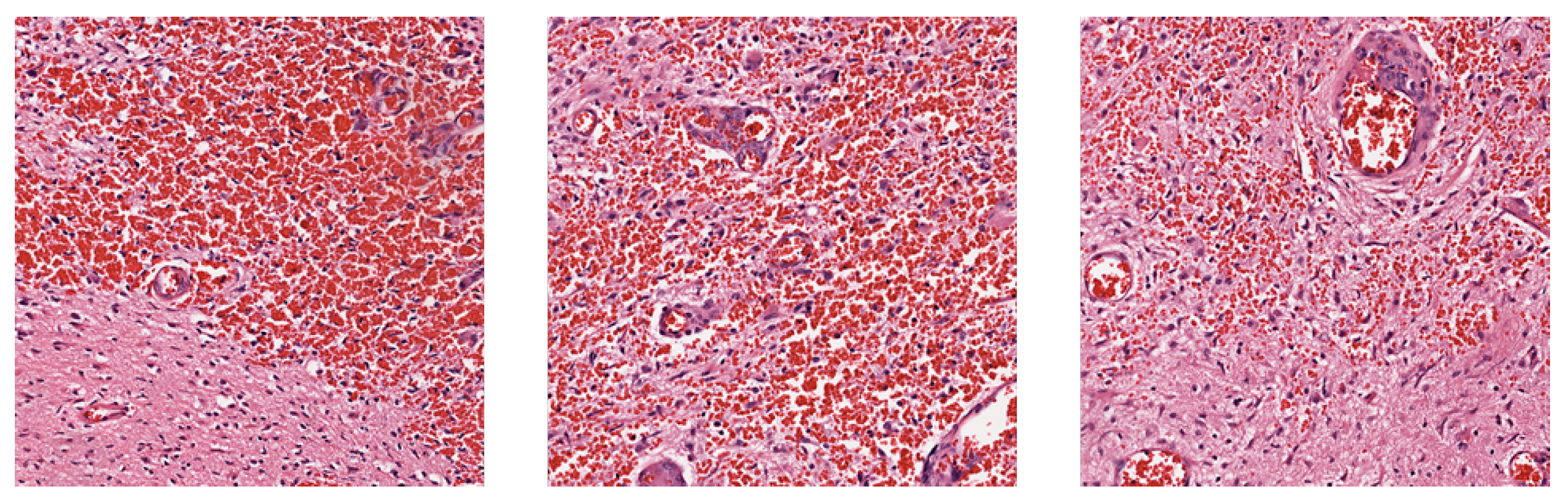Its aggressive nature bears a grade IV classification and a bleak prognosis [1]. Observations in tissue slices of glioblastoma commonly manifest as thrombus formation, microvascular proliferation, and cellular necrosis [2]. However, the tumor’s substantial heterogeneity implies that absence of these phenomena in tissue slices does not preclude the presence of GBM, posing a challenge to accurate prognosis through histological images.

Traditional survival analysis usually relies on manually extracted features modeled using proportional hazard model. For example, Tibshirani (1997) [3] utilized clinical data such as gender, age, and treatment methods, and employed the LASSO method to select pertinent features before inputting into the Cox proportional hazards model. This technique adds a penalty term to the loss function during model computation, constraining outputs within a specific range, thereby retaining essential features and reducing complexity while enhancing predictive efficacy.

Early survival analysis methods have since evolved, leveraging machine learning and deep learning techniques, especially in survival prediction based on whole-slide images (WSIs). However, WSIs are extremely high resolution images; feeding them directly into deep learning models is computationally infeasible. Thus, researchers have proposed methods to extract meaningful patches from WSIs as input. For example, Zhu et al. (2016) [4] addressed the issue by extracting patches from regions of interest (ROIs) annotated by pathologists and trained a deep convolutional neural network (CNN) for lung cancer survival analysis. However, this demands substantial human labor and potentially results in missing insights from other parts of the digital pathology slides.

To mitigate the laborious manual ROI labelling, research studies such as [5,6,7,8,9] have proposed to randomly sample patches from different areas of the WSI. Zhu et al. (2017) [5] then utilized K-means to cluster the sampled patches, and constructed classifiers for each cluster to identify and select the clusters most useful for survival analysis. Li et al. (2018) [6] and Di et al. (2020) [8] constructed a graph or hypergraph as a summarized representation of the WSI by placing feature vectors extracted from the patches as node features, and relational features among the patches as edge features. Li et al. (2023), [10] on the other hand, proposed an entropy-based patch sampling method, and utilized self-supervised learning to alleviate domain gaps from pre-training on natural images. They also introduced an attention-based global-local information fusion strategy to improve prediction accuracy.

However, many of these methods utilized only a fixed subset of all viable patches, even after removing background or distorted patches. Ref. [5] sampled a fixed area ratio of patches from WSI for training. Ref. [7] used only patches from selected clusters to train the main classifier. Ref. [9] sampled a random but fixed 1000 patches from each WSI, while [10] used only patches with high entropy to train the model. By using only a subset of patches for training, these methods may potentially discard important information from the remaining patches.

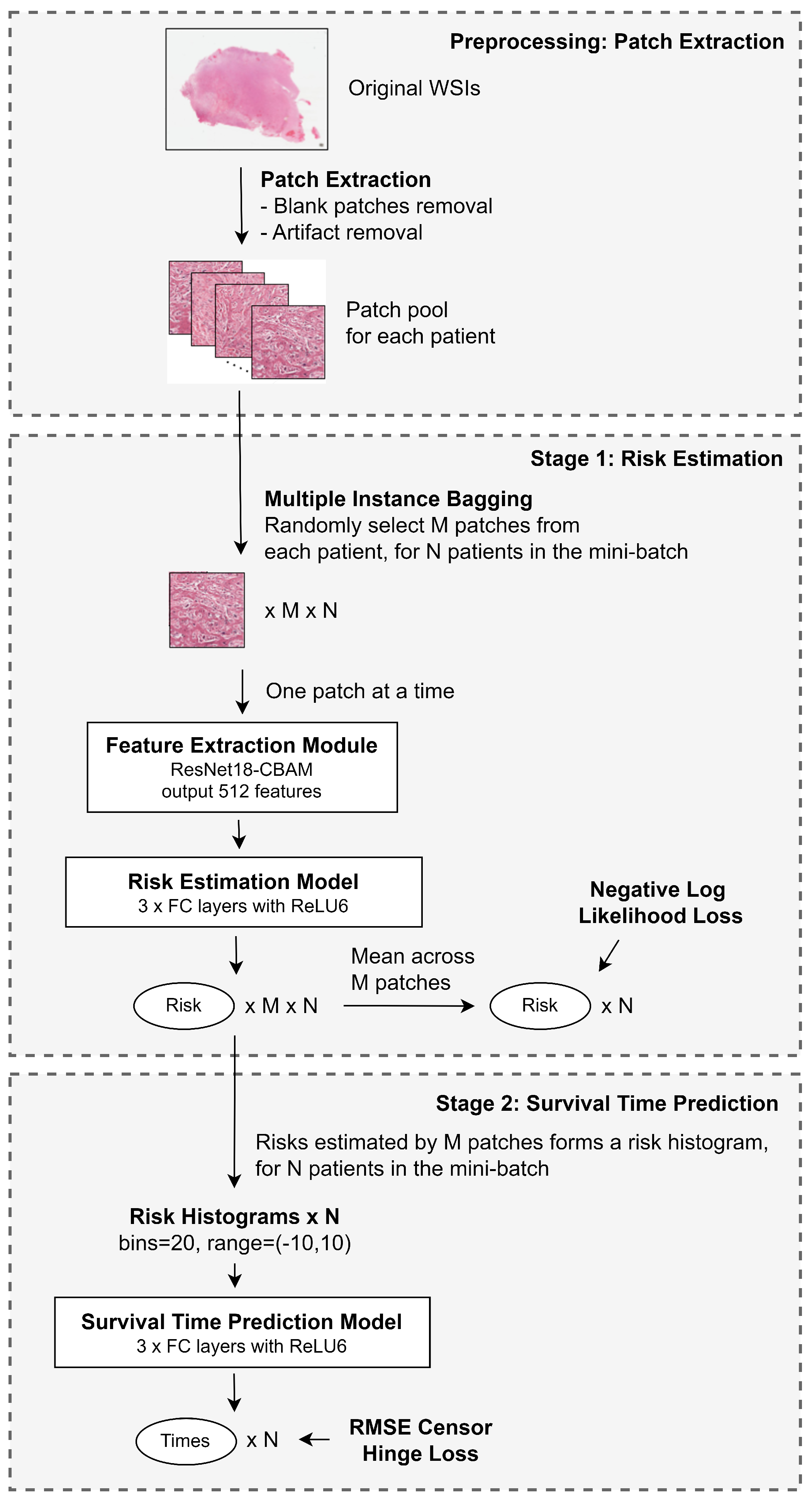
In this study, we propose a method that utilizes all viable patches from the WSI while keeping the training computationally feasible. Additionally, we attempt to predict the exact survival time of patients, beyond the usual risk of death estimation. At the same time, we aim to devise a framework that provides visual explainability for clinicians.

The contributions of this paper can be summarized as follows:

• We introduce a multiple instance bagging strategy that enables the utilization of information from the entire WSI while maintaining computational feasibility during training.
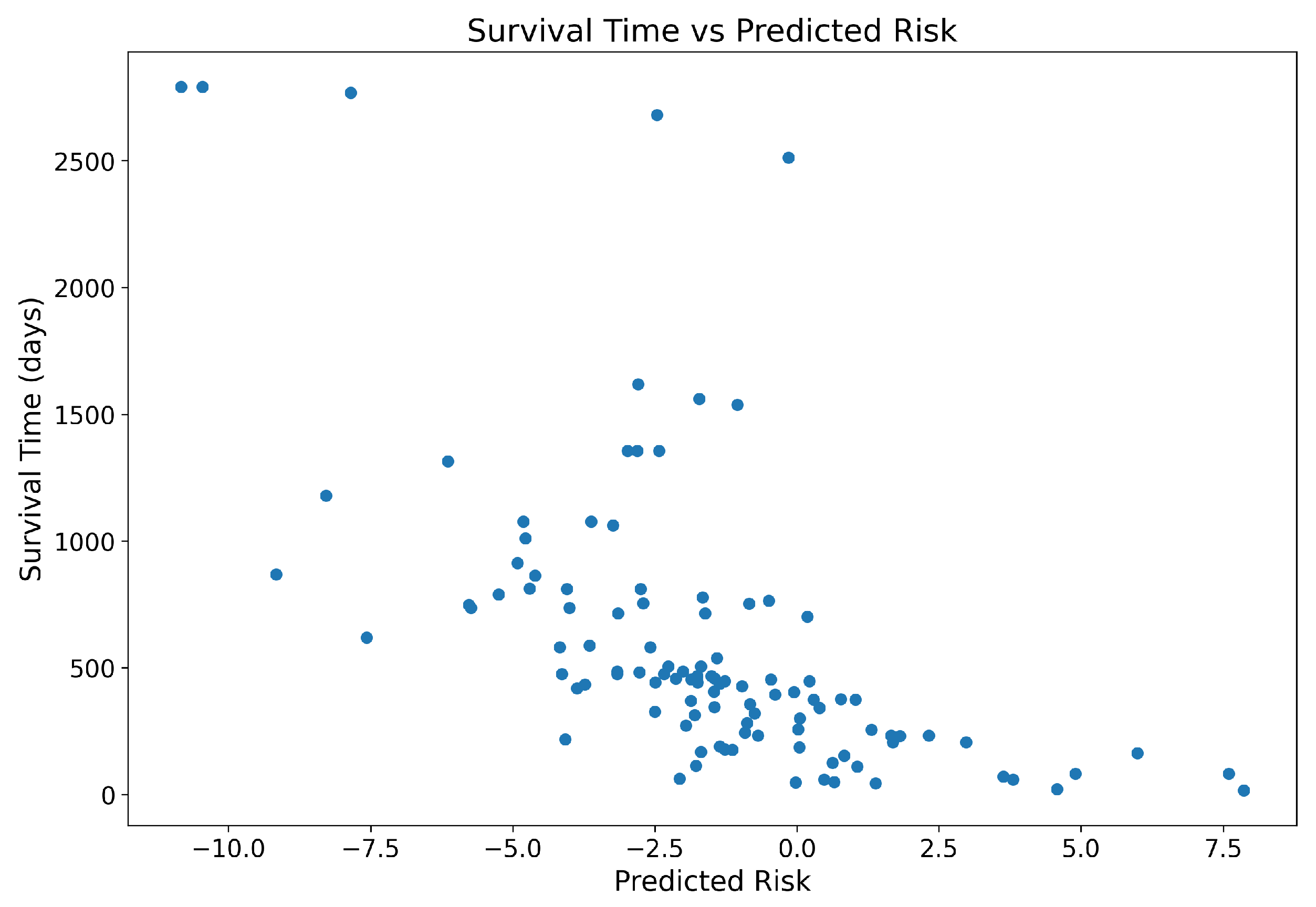
• We develop a two-stage framework that not only estimates survival risk but also predicts actual survival time.
• We propose a new loss function, the Root Mean Square Censor Hinge Loss (RMSCHE), which effectively handles censored data in survival time prediction.
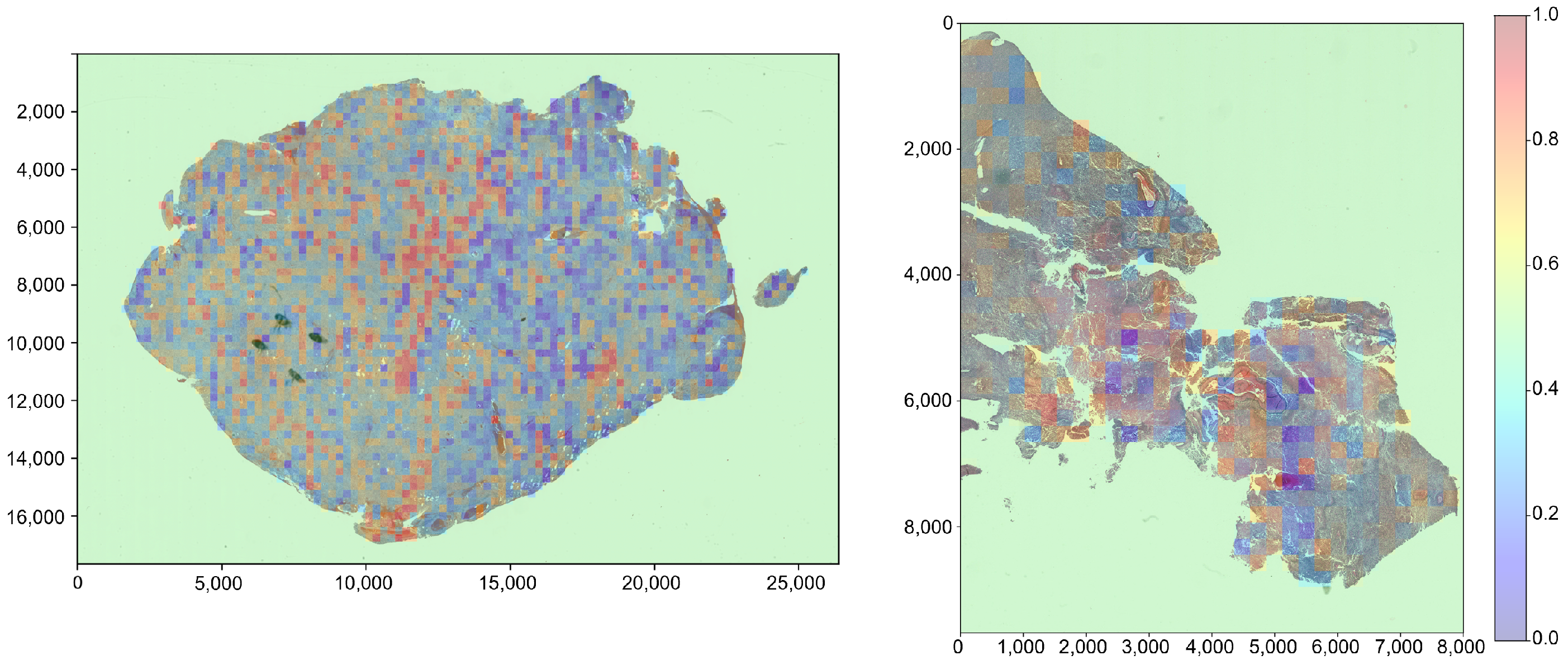
• We implement a heatmap visualization method that provides interpretable risk assessments at the patch level, potentially aiding clinicians in identifying high-risk regions within WSIs.

The rest of the paper is organized as follows: Section 2 introduces the background of survival analysis used in this study. Section 3 outlines the overall framework and details each stage of the proposed method, including patch extraction, risk estimation, and survival time prediction. Section 4 presents the experimental setup, including the dataset, evaluation metrics, and implementation details. We also present the results and discuss the findings in this section. Finally, Section 5 concludes the paper and suggests future research directions.

2. Background

2.1. Survival Analysis

Survival analysis studies the probability of occurrence of a specific event. In the medical context, the event is often defined as patient mortality. However, the presence of censored data, where observed subjects do not experience the event during the study, complicates analyses. The data involved in survival analysis thus includes the feature vectors $\left(x_i\right)$, event or censoring time $\left(t_i\right)$, and an indicator of censoring status ${\delta }_i$. In this study, ${\delta }_i=1$ denotes a patient’s passing during the observation period, with the elapsed time from the study start to the event marked as $t_i$. Conversely, ${\delta }_i=0$ indicates survival through the study, with the duration from the study start to the last recorded data termed as $t_i$ [11].

Survival data are usually modeled in the form of the survival function $S\left(t\right)$ or the hazard function $h\left(t\right)$. The survival function quantifies the cumulative probability of an event not occurring before a specific time, while the hazard function estimates the instantaneous event occurrence probability at a particular time, as shown in (1) and (2), respectively [12], where T is the random variable representing event time.

$$S\left(t\right)=P(T>t)$$

(1)

$$h\left(t\right)=\underset{\Delta t\to 0}{lim}{\displaystyle \frac{P(t\le T<t+\Delta t|t\le T)}{\Delta t}}$$

(2)

To address issues arising from censoring phenomena, three categories of statistical methods have been proposed in the literature: non-parametric, parametric, and semi-parametric models. In this study, we employ the non-parametric Kaplan–Meier method [13] and the semi-parametric Cox proportional hazards model [14] for analysis.

2.2. Kaplan–Meier Method and Cox Proportional Hazards Model

The Kaplan–Meier method does not assume data characteristics, and computes survival probabilities based on the count of patients alive $n_i$ excluding censored patients right before a certain time point $t_i$ and the number of patients experiencing the event $d_i$ at that time [13]. Multiplying the survival probabilities at each time point yields the survival function, as shown in (3).

$$S\left(t\right)=\prod _{i:t_i\le t}{\displaystyle \frac{n_i-d_i}{n_i}}$$

(3)

On the other hand, the Cox proportional hazards model [14] assumes proportional risk functions with respect to explanatory variables, as shown in (4), where $h_0\left(t\right)$ represents baseline hazard.

$$h\left(t\right|x)=h_0\left(t\right)e^{{\mathit{\beta }}^{\mathit{T}}\mathit{x}}$$

(4)

The Cox partial lLikelihood function [15] can be calculated by first estimating an individual’s risk of event occurrence within the cohort at a specific time point using (5), where the summation in the denominator is performed over the set of patients with survival and censored time greater than the time point $t_i$. The Cox partial likelihood function can be obtained by multiplying the individual risk estimates, as shown in (6).

$$l_i\left(\beta \right)={\displaystyle \frac{e^{{\mathit{\beta }}^{\mathit{T}}{\mathit{x}}_{\mathit{i}}}}{{\sum }_{j\in R\left(t_i\right)}{e}^{{\mathit{\beta }}^{\mathit{T}}{\mathit{x}}_{\mathit{j}}}}}$$

(5)

$$l_p\left(\beta \right)=\prod _{i=1}^n{l}_i\left(\beta \right)$$

(6)

The goal is then to find the best parameter $\beta$ that maximizes the Cox partial likelihood function.

2.3. Cox Model in Deep Learning

Contrary to classification models, survival risk prediction models do not compare predictions with ground truth; instead, they consider the order of predicted risk values related to survival times, taking into account the censoring status.

By taking the logarithm of the Cox partial likelihood function in (6), the Cox partial log-likelihood function is obtained, as shown in (7), which transforms the product of risk estimates into a summation of risk values.

$$L_p\left(\beta \right)=logl\left(\beta \right)=\sum _{i=1}^n\left[{\mathit{\beta }}^{\mathit{T}}{\mathit{x}}_{\mathit{i}}-log\left(\sum _{j\in R\left(t_i\right)}{e}^{{\mathit{\beta }}^{\mathit{T}}{\mathit{x}}_{\mathit{j}}}\right)\right]$$

(7)

In deep learning, gradient descent is commonly used to optimize model parameters. To find the best parameter $\beta$ that maximizes the Cox partial log-likelihood function, we take the negative of the function, as shown in (8), and minimize it instead. This gives the loss function for the survival risk prediction model.

$$\mathrm{Loss}\mathrm{function}=C\left(\beta \right)=-\sum _{i=1}^n\left[{\mathit{\beta }}^{\mathit{T}}{\mathit{x}}_{\mathit{i}}-log\left(\sum _{j\in R\left(t_i\right)}{e}^{{\mathit{\beta }}^{\mathit{T}}{\mathit{x}}_{\mathit{j}}}\right)\right]$$

(8)

3. Methodology

3.1. Framework

The proposed framework includes a preprocessing stage and a two-stage prediction stage, as illustrated in Figure 1. First, we cut the entire WSI into non-overlapping patches using a sliding window approach. These patches are then tested for background and blurriness, and removed if they do not meet certain criteria.

A unique multiple instance bagging patch selection method was proposed to randomly select different subsets of patches from each WSI in each epoch of training, thus keeping the training computationally feasible while leveraging information from the entire WSI. A feature extraction module can be trained using these patches, and the extracted features serve as input data for further analysis.

Unlike traditional survival analysis methods that focus solely on estimating risk, our framework directly predicts both the survival risk and the actual survival time, which provides a more interpretable output for clinicians and patients. The two-stage prediction model includes two main components:

• A risk estimation model based on the features extracted by the feature extraction module that outputs a risk score for each patch. These risk scores are then averaged to obtain a single estimated risk score for each WSI.
• A time prediction model that takes the histogram of patch-wise risk predictions as input and estimates the survival time.

Both the risk estimation and time prediction models utilized a multilayer perceptron (MLP) architecture, each comprised of three fully connected layers separated by ReLU6 activation functions.

In the following subsections, we detail each stage of the proposed framework.

3.2. Preprocessing: Patch Extraction

The patch extraction approach was as follows: first, utilizing a sliding window of size $256\times 256$, patches were extracted from the original WSI without overlap. Then, patches that were mostly blank or containing artifacts were detected and removed. Finally, the remaining patches were saved as a patch pool for each patient. The whole patch extraction process was automatic once the thresholds had been set. For each WSI, thousands of patches were extracted.

3.2.1. Blank Patches Removal

In medical imaging, WSIs often contain extensive blank regions that do not contribute to model learning. We applied a serie of morphological operations (dilation with kernel (3, 3), closing with kernel (20, 20), and opening with kernel (15, 15)) on masks generated by converting RGB tissue images to HSV color space and segmenting ranges of HSV values above (156, 43, 46) to emphasize regions with tissue. Patches that had 0.5 or less tissue coverage ratio were filtered away. Examples are shown in Figure 2.

3.2.2. Artifact Detection

We observed that some WSIs provided in the dataset had marker drawings. When extracted into patches, these marker drawings covered a large area of the patches, leading to altered color or diminished contrast. To detect these affected patches, we employed the Laplacian edge detection method [16] provided by OpenCV on grayscale patch images generated using the COLOR_BGR2GRAY method [17,18] to identify edges within the patches. Regions affected by markings tend to have fewer edges detected due to reduced contrast. The variance of output images was calculated as an indicator of edge presence. Patches that had a calculated variance less than 300 were considered as affected and removed. Examples are shown in Figure 3.

3.3. Stage 1: Risk Estimation

3.3.1. Multiple Instance Bagging

Most studies adopt random sampling, ROI-based patch selection strategies, or heuristics to select only a subset of potentially informative patches for training. Our approach is different. We propose a multiple instance bagging strategy where, in each epoch, a different subset of M patches are randomly selected from each patient’s pool of extracted patches. This sets the number of patches utilized in each epoch, thus keeping the training computationally feasible. Concurrently, the model is allowed to learn from different representations of the same WSI across epochs, reducing the risk of overfitting to specific regions and enhancing the model’s ability to generalize. Note that this number M is also utilized in the survival time prediction stage, where the risk histogram is calculated based on the predicted risk values from the selected M patches. The M value thus cannot be too small for effective construction of a risk histogram. We set M as 16 for this study to keep the computational cost within the limit of GPU memory, while still allowing a reasonable risk histogram to be constructed.

3.3.2. Feature Extraction Module

The base model for feature extraction was the residual attention model proposed by Woo et al. [19]. The major component of this residual attention model is the convolutional block attention module (CBAM), which combines both channel and spatial attention modules, thus selectively extracting features from different channel characteristics and spatial pixel relationships. The residual attention model injects the CBAM modules into ResNet18 model architecture, enhancing essential information within each residual block and demonstrating reduced error rates on ImageNet classification tasks [19]. A schematic diagram of the model is shown in Figure 4.

In this study, the feature extraction module began with pre-trained weights on ImageNet. The module processed the selected patches obtained from the patch extraction stage described in Section 3.2, yielding 512 features as output for subsequent stages.

3.3.3. Risk Estimation Model

To train the risk estimation model, we employed the negative log-likelihood loss function based on the Cox proportional hazards model, as described in Equations (9) and (10).

In a batch-wise training routine for the risk estimation model, we estimated the population distribution by considering a batch of N patients, where $y_i={\mathit{\beta }}^{\mathit{T}}{\mathit{x}}_{\mathit{i}}$ is the model prediction and $t_i$ the actual survival time for patient i. The loss function could then be computed as shown in (9).

$$\mathrm{Loss}\mathrm{function}=C\left(\beta \right)=-\sum _{i=1}^N\left[y_i-log\left(\sum _{j\in R\left(t_i\right)}{e}^{y_j}\right)\right]$$

(9)

By taking the derivative of (9) with respect to $\beta$, we obtained the gradient function required for parameter updates during model training, as shown in (10).

$${\displaystyle \frac{\partial C\left(\beta \right)}{\partial \beta }}=-\sum _{i=1}^N\left[{\mathit{x}}_{\mathit{i}}-{\displaystyle \frac{{\sum }_{j\in R\left(t_i\right)}{\mathit{x}}_{\mathit{j}}{e}^{y_j}}{{\sum }_{j\in R\left(t_i\right)}{e}^{y_j}}}\right]$$

(10)

The risk estimation model was a simple MLP model made of three fully connected layers with output nodes of 32, 16, and 1, respectively, and ReLU6 activation functions. It took in the 512 features extracted by the feature extraction module as input, and output a risk score for each patch. This set of M risk scores were used for the following survival time prediction stage. These M risk scores were also averaged to estimate the risk score for a given WSI, which was the final output of the risk estimation model and was used for loss calculation.

3.4. Stage 2: Survival Time Prediction

3.4.1. Risk Histogram-Based Survival Time Prediction

Given the risk scores produced from the risk estimation stage, we aimed to predict the actual survival time of patients. A straight forward approach would be to put the final average risk score through a simple multilayer perceptron (MLP) regression model and output a survival time prediction. However, this would discard the rich information that could be hidden in the specific distribution of risk scores of the patches. Additionally, we aimed to create a survival time prediction model that can take in any number of risk scores from patches, not just a fixed number dictated by the M value. This allowed the model to perform inference on different WSIs with varying number of patches, using all the patches extracted from each WSI.

To accomplish this, we proposed using the risk histogram as input to train the survival time prediction model. The risk histogram was constructed by arranging the risk scores obtained from the patches into 20 bins in the range −10 to 10. The histogram was then normalized to obtain a probability density function, which had two desired properties:

• The histogram had a fixed size (20 bins in this case), which could serve as an input with fixed input size for the survival time prediction model to process.
• Due to the normalization, the histogram was able to take in risk scores from any number of patches, not just a fixed number dictated by the M value.

The survival time prediction model is a simple MLP model similar to the risk estimation model. It takes in the risk histogram as input and outputs the predicted survival time.

Note that the risk estimation model and the survival time prediction model were trained using separate optimizers.

3.4.2. Root Mean Square Censor Hinge Loss

A challenge in survival time prediction is in handling the censored data, where the event of interest is not observed. Without the actual survival times, we cannot employ the usual mean square error loss function for model learning. One may choose to ignore the censored cases and only consider the observed ones when training the survival time prediction model. However, this throws away valuable information from the censored cases.

To fully utilize the information from both observed and censored cases, we proposed a novel loss function called the Root Mean Square Censor Hinge Loss (RMSCHE), or censor hinge loss for short. The censor hinge loss is based on the observation that, while the actual survival time is not known, the follow-up time provides the information that the patient is at least alive up to that time. We can thus utilize a hinge loss approach similar to that used in support vector machine models, where the loss is only incurred when the predicted time is shorter than the follow-up time, as shown in (11), where N is the number of samples, ${\delta }_i$ is the event indicator (1 for observed, 0 for censored), $t_i$ is the true survival or censoring time, and ${\widehat{t}}_i$ is the predicted survival time.

$$L_{RMSCHE}=\sqrt{{\displaystyle \frac{1}{N}}\sum _{i=1}^N{\delta }_i{({\widehat{t}}_i-t_i)}^2+(1-{\delta }_i)max{(0,{\widehat{t}}_i-t_i)}^2},$$

(11)

For observed events, this loss function calculates the standard root mean square error. For censored events, it only incurs a loss when the predicted time is shorter than the censoring time, using a hinge loss formulation. This approach allows the model to learn from both observed and censored data while respecting the partial information provided by censored cases.

3.5. Heatmap Visualization

One unique feature of our framework is the ability to visualize the risk scores of patches from the same WSI as a heatmap, providing interpretable information for clinicians. This is possible because the risk estimation model was designed to take in the patches one at a time. Although during training we only utilized M patches from each WSI in each epoch, the risk estimation model is capable of taking in inputs of any number of patches. Therefore, for a given test WSI, we can feed all its extracted patches into the trained risk estimation model and obtain the risk scores for all patches. By piecing together the risk scores from all patches back into the original WSI size, we can overlay the risk scores as a heatmap onto the original WSI for visual inspection. This displays regions that predict higher or lower risk, which translates to regions that predicts worse or better survival outcomes, providing interpretable information for further inspection by clinicians.

The process can be summarized as follows:

• For a given test WSI, we extracted all possible patches using a sliding window approach.
• Each patch was then inputted into the trained risk estimation model to obtain patch-wise risk predictions.
• The predicted risk values for all patches were combined and overlaid onto the original WSI, creating a risk heatmap.

An example of the heatmap is shown in Figure 5.

4. Results and Discussion

4.1. Database Introduction

The study utilized images from the publicly available dataset sourced from The Cancer Genome Atlas Program (TCGA), specifically focusing on digital pathology slides of glioblastoma multiforme (GBM) patients [20]. Each image in this dataset underwent scanning at three different magnification levels. For this research, $256\times 256$ patches were extracted at $20\times$ magnification for model training, with examples shown in Figure 6.

Excluding slides that could not be read, we utilized 544 WSIs from 247 individuals. The split ratio between training and testing datasets was 8:2, as shown in

Table 1. Number of WSIs.

	No. WSIs
Train	435
Test	109
Total	544

.

4.2. Hardware and Software Environment

The hardware setup employed for this study is detailed in

Table 2. Hardware specifications.

Hardware	Specifications
Operating System (OS)	Windows 11
Central Processing Unit (CPU)	Intel(R) Core(TM) i7-14700 @ 2.10 GHz
Graphics Processing Unit (GPU)	NVIDIA GeForce RTX 4080 SUPER, ASUSTeK, Taiwan
Random Access Memory (RAM)	DDR4 32 GB $\times 2$, Kingston, NY, USA

. Given the large size of digital pathology slide images, we utilized OpenSlide [21], a C library specialized in WSI retrieval which enables access to images at different magnifications.

Table 3. Software environment.

Software	Version
Python Version	3.11.9
PyTorch Version	2.4.1
CUDA Version	11.8
Development Environment	VS Code 1.93.1
OpenSlide Version	3.4.1

outlines the software environment.

4.3. Training Parameter Configuration

Table 4. Hyperparameter settings.

Hyperparameter	Settings
Epochs	500
Batch size (N)	16
Number of patches (M)	16
Patch size	$256\times 256$
Optimizer—risk estimation	Adam
Optimizer—survival time prediction	Adam
Learning rate—risk estimation	0.00005
Learning rate—survival time prediction	0.00005
Loss function—risk estimation	Negative Log Partial Likelihood
Loss function—survival time prediction	Root Mean Square Censor Hinge Loss

summarizes the training hyperparameters utilized in this study.

4.4. Evaluation Metrics

For risk estimation, we employed the concordance index (C-Index) to evaluate the efficacy of the model, aligning with the existing literature. For survival time prediction, we employed the Root Mean Square Error (RMSE) and Mean Absolute Error (MAE) metrics.

4.4.1. Concordance Index (C-Index)

In survival risk prediction research, the C-Index is commonly used. The C-Index is computed by taking pairs of patients and comparing the predicted survival risk values with the actual survival times. If the patient with the higher survival risk value matches a shorter actual survival time, the pair is considered concordant. The C-Index is then calculated by dividing the number of concordant pairs by the total number of comparable pairs, as shown in (12). The pairs are considered comparable if both patients are not censored, or if the patient with shorter observed survival time experienced the event [22]. Note that the C-Index measures how consistent is the model’s predicted ranking of patient risks with the ranking of actual survival times.

$$\mathrm{C}\text{-}\mathrm{Index}={\displaystyle \frac{\mathrm{Number}\mathrm{of}\mathrm{concordant}\mathrm{pairs}}{\mathrm{Number}\mathrm{of}\mathrm{comparable}\mathrm{pairs}}}$$

(12)

The C-Index ranges between 0.5 and 1. A value of 0.5 indicates random predictions, implying the model lacks predictive capability, while a value of 1 signifies complete consistency between predictions and reality. The C-Index calculation takes into account both normal and censored data, which is crucial in real clinical scenarios.

4.4.2. Log Rank Test

The log-rank Test, first introduced by Mantel in 1966 [23], evaluates differences between survival curves of distinct groups. The null hypothesis assumes no difference between survival curves of the two groups. By summing observed and expected event numbers, the test computes a statistic used to determine significant differences between survival curves.

The log-rank test begins by first calculating the expected number of survivals for each group at each time point, which can be estimated by multiplying the survival probability with the number of subjects at risk in each group. Then, by summing this expected number of events for each group across all event time, we obtain the total number of expected events E for each group, which can then be compared with the total observed number of events O for each group, as shown in (13) for the group 2 case, where $d_i$ and $r_i$ are the number of events and number of subjects at risk at time $t_i$ across all groups, and $r_{2i}$ is the number of subjects at risk in group 2 at time $t_i$.

$$E_2=\sum _{i=1}^k{\displaystyle \frac{d_i}{r_i}}{r}_{2i}$$

(13)

The test statistic calculated by (14) follows a ${\chi }^2$ distribution with 1 degree of freedom, where $O_1$ and $O_2$ are the total observed number of events for group 1 and group 2, and $E_1$ and $E_2$ are the total expected number of events for group 1 and group 2, respectively [24,25].

$${\chi }^2={\displaystyle \frac{{(O_1-E_1)}^2}{E_1}}+{\displaystyle \frac{{(O_2-E_2)}^2}{E_2}}$$

(14)

In this study, we utilize the log-rank test to test the null hypothesis for a p-value below 0.005, that is, to determine whether a significant difference can be found between the survival curves of predicted high-risk and low-risk groups plotted using the Kaplan–Meier method as another measure of model performance. The Python package lifeline was utilized for the calculation of this log-rank test statistic [26].

4.4.3. Root Mean Square Error (RMSE) and Mean Absolute Error (MAE) for Survival Time Prediction

To optimize the model’s learning, we normalized the survival time to a range between 0 and 1 by dividing the survival time by the maximum survival time in the dataset (3881 days). This normalized survival time was used to calculate the RMSE and MAE between the predicted survival time and the actual survival time. To obtain an estimate of the prediction error in days, we multiplied the RMSE and MAE by 3881 days to convert it back to the original scale in days.

It is worth noting that, while RMSE is useful during model training due to its differentiable property, it tends to be more sensitive to outliers when used as a performance metric. Therefore, we included the MAE as another metric to provide a more comprehensive evaluation of the model’s performance.

4.5. Experimental Results

4.5.1. Risk Estimation

To present a more comprehensive evaluation of the model’s performance, we performed the experiment ten times with different random seeds. The performance metrics were then averaged, as shown in Figure 7. Due to the random nature in patch selection across different epochs, we also performed Gaussian smoothing with a window size of 10 epochs to present a more meaningful learning trajectory.

At the best performing epoch (epoch 490), the framework yielded a very promising result, with a C-Index of $73.16\pm 2.15\%$.

4.5.2. Survival Time Prediction

Using the result from the best performing model, we plotted the actual survival time against the predicted risk, as shown in Figure 8. A clear negative correlation can be observed, indicating that the model was able to learn the relationship between the predicted risk and survival times, with a Pearson correlation coefficient of −0.6027.

This motivated us in training the survival time prediction model given the predicted risks, which yielded a very promising result, as seen in the plot of predicted survival time against actual survival time in Figure 9. The dots lie close to the identity line, indicating that the model was able to translate the predicted risk to survival time, albeit with some outliers. The Pearson correlation coefficient between survival time and predicted survival time was 0.6602.

The RMSE and MAE between the actual survival time and predicted survival time were 448.03 and 260.19 days, respectively, as presented in

Table 5. Survival time prediction performance.

Metric	Value
RMSE	448.03 days
MAE	260.19 days

.

As can be seen from Figure 10, the distribution of original survival time concentrates in the range between 0 to 1000 days, with the mean difference between any pairs of survival times at about 560 days. As a result, it may seem that the achieved RMSE of 448 days is not very useful; however, we note that the RMSE is sensitive to outliers. Thus, by also presenting the MAE, we can see that a MAE of 260 days is indeed a large improvement from random guessing, indicating the potential for direct survival time prediction.

The survival time prediction performance can be further validated using the plot of sorted absolute error against sample percentile in Figure 11. It can be seen that most of the absolute error concentrates in the higher percentiles. For nearly 80% of the samples, the absolute error is less than 400 days, indicating that the model is able to predict the survival time with a reasonable degree of accuracy.

4.5.3. Generating Kaplan–Meier Survival Curves Using Predicted Results

We split the dataset based on median of predicted risk values into high-risk and low-risk groups, and generated two distinct survival curves using the Kaplan–Meier method, as shown in Figure 12. The resulting survival curves demonstrated significant differences between high=risk and low-risk groups using the log-rank test, with a p-value of $3.88\times {10}^{-9}$, well below the usual threshold of 0.005.

4.5.4. Comparison with Related Literature

In comparison with recent studies that have also used the glioblastoma dataset from TCGA, this research demonstrated promising predictive performance, as presented in

Table 6. Comparison with the related literature.

Author	Methods	C-Index
Zhu et al. (2016) [4]	DeepConvSurv	62.9%
Zhu et al. (2017) [5]	WSISA	64.5%
Li et al. (2018) [6]	DeepGraphSurv	63.5%
Tang et al. (2019) [7]	CapSurv	67.0%
Di et al. (2020) [8]	RankSurv	66.2 %
Fan et al. (2023) [9]	ConsistSurv with SSL	67.0%
Li et al. (2023) [10]	MSFN	69.1%
This Study		$73.16\pm 2.15\%$

. Notably, the proposed model achieved a significantly higher C-Index at $73.16\pm 2.15\%$.

4.5.5. Comparison of Model Parameters

As depicted in

Table 7. Comparison of model parameters.

Methods	Model Size	Ave. Inf. Time (s)
MSFN	723,208,234	0.190
Ours	11,301,200	0.027

, when we compare with the state-of-the-art MSFN model proposed by Li et al. (2022) [10], the framework proposed in this study notably reduced the parameter amount by approximately 98% and used only one-seventh the inference time per WSI sample.

5. Conclusions

This study presented a novel framework for glioblastoma multiforme (GBM) survival analysis using whole-slide images (WSIs). Our approach addressed several key challenges in the field. First, we introduced a multiple instance bagging strategy that enabled the utilization of information from the entire WSI while maintaining computational feasibility during training. A two-stage framework that goes beyond estimating survival risk by also predicting the actual survival time was proposed. To address the censored data in survival time prediction, we proposed the Root Mean Square Censor Hinge Loss (RMSCHE), yielding promising results. Finally, our framework enabled the implementation of heatmap visualization, which offers a bridge between complex deep learning models and clinical interpretability. By color-coding risk assessments at the patch level, this method allows for intuitive identification of potentially problematic regions within tissue samples, which could increase trust and adoption of such models in medical practice.

Our experiments on the TCGA-GBM dataset demonstrated the effectiveness of the framework, achieving a concordance index (C-Index) of $73.16\pm 2.15\%$, outperforming existing methods in the literature. The log-rank test based on Kaplan–Meier survival curves showed a statistically significant separation between predicted high-risk and low-risk groups (p < 0.005), further validating the model’s discriminative power. For survival time prediction, our framework achieved a RMSE of 448 days and a MAE of 260 days. Comparing to the mean survival time difference between any two patients in the dataset, that is, 560 days, the model showed promising predictive value. Notably, our framework achieved these results while using much fewer parameters compared to state-of-the-art methods, reducing the model size by approximately 98% and decreasing average inference time per WSI by about 86%. This efficiency makes our approach more feasible for practical clinical applications.

While this study demonstrates promising results, there are several avenues for future research. First, investigating fully unsupervised patch selection methods could reduce the need for manual threshold setting, potentially improving the model’s adaptability to diverse datasets. Second, integrating multi-modal data, including clinical information and radiological images, could provide a more comprehensive view of patient prognosis. Owing to advancements in genetic testing technologies, several studies have confirmed that differences exist in the patterns of gene expression useful for the prognosis of GBM patients [27,28]. Incorporating these genetic data as features during survival risk prediction model development might further enhance predictive capabilities and offer insights into the molecular mechanisms underlying GBM progression. Finally, the dataset used in this study does not indicate whether death is due to glioblastoma or other causes, which introduces competing risks that should be considered in future models.

References

1. Hanif, F.; Muzaffar, K.; Perveen, k.; Malhi, S.; Simjee, S. Glioblastoma Multiforme: A Review of Its Epidemiology and Pathogenesis through Clinical Presentation and Treatment. Asian Pac. J. Cancer Prev. 2017, 18, 3. [Google Scholar] [CrossRef] [PubMed]
2. Yu, K.H.; Zhang, C.; Berry, G.J.; Altman, R.B.; Ré, C.; Rubin, D.L.; Snyder, M. Predicting Non-Small Cell Lung Cancer Prognosis by Fully Automated Microscopic Pathology Image Features. Nat. Commun. 2016, 7, 12474. [Google Scholar] [CrossRef] [PubMed]
3. Tibshirani, R. THE LASSO METHOD FOR VARIABLE SELECTION IN THE COX MODEL. Stat. Med. 1997, 16, 385–395. [Google Scholar] [CrossRef]
4. Zhu, X.; Yao, J.; Huang, J. Deep Convolutional Neural Network for Survival Analysis with Pathological Images. In Proceedings of the 2016 IEEE International Conference on Bioinformatics and Biomedicine (BIBM), Shenzhen, China, 15–18 December 2016; pp. 544–547. [Google Scholar] [CrossRef]
5. Zhu, X.; Yao, J.; Zhu, F.; Huang, J. WSISA: Making Survival Prediction from Whole Slide Histopathological Images. In Proceedings of the 2017 IEEE Conference on Computer Vision and Pattern Recognition (CVPR), Honolulu, HI, USA, 22–25 July 2017; pp. 6855–6863. [Google Scholar] [CrossRef]
6. Li, R.; Yao, J.; Zhu, X.; Li, Y.; Huang, J. Graph CNN for Survival Analysis on Whole Slide Pathological Images. In Medical Image Computing and Computer Assisted Intervention—MICCAI 2018; Frangi, A.F., Schnabel, J.A., Davatzikos, C., Alberola-López, C., Fichtinger, G., Eds.; Springer International Publishing: Cham, Switzerland, 2018; Volume 11071, pp. 174–182. [Google Scholar] [CrossRef]
7. Tang, B.; Li, A.; Li, B.; Wang, M. CapSurv: Capsule Network for Survival Analysis With Whole Slide Pathological Images. IEEE Access 2019, 7, 26022–26030. [Google Scholar] [CrossRef]
8. Di, D.; Li, S.; Zhang, J.; Gao, Y. Ranking-Based Survival Prediction on Histopathological Whole-Slide Images. In Medical Image Computing and Computer Assisted Intervention—MICCAI 2020; Martel, A.L., Abolmaesumi, P., Stoyanov, D., Mateus, D., Zuluaga, M.A., Zhou, S.K., Racoceanu, D., Joskowicz, L., Eds.; Springer International Publishing: Cham, Switzerland, 2020; Volume 12265, pp. 428–438. [Google Scholar] [CrossRef]
9. Fan, L.; Sowmya, A.; Meijering, E.; Song, Y. Cancer Survival Prediction From Whole Slide Images With Self-Supervised Learning and Slide Consistency. IEEE Trans. Med. Imaging 2023, 42, 1401–1412. [Google Scholar] [CrossRef] [PubMed]
10. Li, L.; Liang, Y.; Shao, M.; Lu, S.; Liao, S.; Ouyang, D. Self-Supervised Learning-Based Multi-Scale Feature Fusion Network for Survival Analysis from Whole Slide Images. Comput. Biol. Med. 2023, 153, 106482. [Google Scholar] [CrossRef]
11. Kartsonaki, C. Survival Analysis. Diagn. Histopathol. 2016, 22, 263–270. [Google Scholar] [CrossRef]
12. Clark, T.G.; Bradburn, M.J.; Love, S.B.; Altman, D.G. Survival Analysis Part I: Basic Concepts and First Analyses. Br. J. Cancer 2003, 89, 232–238. [Google Scholar] [CrossRef] [PubMed]
13. Goel, M.K.; Khanna, P.; Kishore, J. Understanding Survival Analysis: Kaplan-Meier Estimate. Int. J. Ayurveda Res. 2010, 1, 274–278. [Google Scholar] [CrossRef] [PubMed]
14. Cox, D.R. Regression Models and Life-Tables. J. R. Stat. Soc. Ser. (Methodol.) 1972, 34, 187–220. [Google Scholar] [CrossRef]
15. Hosmer, D.W.; Lemeshow, S.; May, S. Applied Survival Analysis: Regression Modeling of Time-to-Event Data, 2nd ed.; Wiley Series in Probability and Statistics; Wiley-Interscience: Hoboken, NJ, USA, 2008. [Google Scholar]
16. Gonzalez, R.C.; Woods, R.E.; Eddins, S.L. Digital Image Processing Using MATLAB; Pearson/Prentice Hall: Upper Saddle River, NJ, USA, 2004. [Google Scholar]
17. OpenCV: Laplace Operator. Available online: https://docs.opencv.org/3.4/d5/db5/tutorial_laplace_operator.html (accessed on 1 February 2024).
18. OpenCV: Color Conversions. Available online: https://docs.opencv.org/3.4/de/d25/imgproc_color_conversions.html#color_convert_rgb_gray (accessed on 1 September 2024).
19. Woo, S.; Park, J.; Lee, J.Y.; Kweon, I.S. CBAM: Convolutional Block Attention Module. In Computer Vision—ECCV 2018; Ferrari, V., Hebert, M., Sminchisescu, C., Weiss, Y., Eds.; Springer International Publishing: Cham, Switzerland, 2018; Volume 11211, pp. 3–19. [Google Scholar] [CrossRef]
20. Scarpace, L.; Mikkelsen, T.; Cha, S.; Rao, S.; Tekchandani, S.; Gutman, D.; Saltz, J.H.; Erickson, B.J.; Pedano, N.; Flanders, A.E.; et al. The Cancer Genome Atlas Glioblastoma Multiforme Collection (TCGA-GBM) (Version 5) [Data set]. 2016. Available online: https://www.cancerimagingarchive.net/collection/tcga-gbm/ (accessed on 1 September 2022).
21. Goode, A.; Gilbert, B.; Harkes, J.; Jukic, D.; Satyanarayanan, M. OpenSlide: A Vendor-Neutral Software Foundation for Digital Pathology. J. Pathol. Informatics 2013, 4, 27. [Google Scholar] [CrossRef] [PubMed]
22. Sksurv.Metrics. Concordance_index_censored—Scikit-Survival 0.22.2. Available online: https://scikit-survival.readthedocs.io/en/stable/api/generated/sksurv.metrics.concordance_index_censored.html (accessed on 1 February 2024).
23. Mantel, N. Evaluation of Survival Data and Two New Rank Order Statistics Arising in Its Consideration. Cancer Chemother. Rep. 1966, 50, 163–170. [Google Scholar] [PubMed]
24. Bland, J.M.; Altman, D.G. The Logrank Test. BMJ Br. Med. J. 2004, 328, 1073. [Google Scholar] [CrossRef] [PubMed]
25. Bewick, V.; Cheek, L.; Ball, J. Statistics Review 12: Survival Analysis. Crit. Care 2004, 8, 389–394. [Google Scholar] [CrossRef] [PubMed]
26. Davidson-Pilon, C. Lifelines: Survival Analysis in Python. J. Open Source Softw. 2019, 4, 1317. [Google Scholar] [CrossRef]
27. Farsi, Z.; Allahyari Fard, N. The Identification of Key Genes and Pathways in Glioblastoma by Bioinformatics Analysis. Mol. Cell. Oncol. 2023, 10, 2246657. [Google Scholar] [CrossRef] [PubMed]
28. Zhu, X.; Pan, S.; Li, R.; Chen, Z.; Xie, X.; Han, D.; Lv, S.; Huang, Y. Novel Biomarker Genes for Prognosis of Survival and Treatment of Glioma. Front. Oncol. 2021, 11, 667884. [Google Scholar] [CrossRef] [PubMed]
Figure 1. The proposed framework.
Information 15 00750 g001
Figure 2. These patches with less than 0.5 tissue coverage ratio were removed.
Information 15 00750 g002
Figure 3. Patches with less than 300 detected edge variance were removed.
Information 15 00750 g003
Figure 4. Residual attention model.
Information 15 00750 g004
Figure 5. Visualizing risk scores as heatmap. Red and blue colors indicate higher and lower risk, respectively.
Information 15 00750 g005
Figure 6. Example patches extracted from the dataset.
Information 15 00750 g006
Figure 7. Learning trajectories of the average C-Indexes across 10 runs. The shaded area indicates the maximum and minimum values.
Information 15 00750 g007
Figure 8. Actual survival time vs predicted risk.
Information 15 00750 g008
Figure 9. Predicted survival time vs actual survival time.
Information 15 00750 g009
Figure 10. Survival time histogram.
Information 15 00750 g010
Figure 11. Sorted absolute error against sample percentile.
Information 15 00750 g011
Figure 12. Kaplan–Meier survival curves plotted based on median predicted survival risk.
Information 15 00750 g012