Is Short-Term Memory Made of Two Processing Units? Clues from Italian and English Literatures down Several Centuries

Abstract

We propose that short-term memory (STM), when processing a sentence, uses two independent units in series. The clues for conjecturing this model emerge from studying many novels from Italian and English Literature. This simple model, referring to the surface of language, seems to describe mathematically the input-output characteristics of a complex mental process involved in reading/writing a sentence. We show that there are no significant mathematical/statistical differences between the two literary corpora by considering deep-language variables and linguistic communication channels. Therefore, the surface mathematical structure of alphabetical languages is very deeply rooted in the human mind, independently of the language used. The first processing unit is linked to the number of words between two contiguous interpunctions, variable Ip, approximately ranging in Miller’s 7 ± 2 range; the second unit is linked to the number of Ip’s contained in a sentence, variable M_F, ranging approximately from 1 to 6. The overall capacity required to process a sentence fully ranges from 8.3 to 61.2 words, values that can be converted into time by assuming a reading speed, giving the range 2.6∼19.5 s for fast-reading and 5.3∼30.1 s for the average reader. Since a sentence conveys meaning, the surface features we have found might be a starting point to arrive at an information theory that includes meaning.

1. Short-Term Memory Capacity Can Be Estimated from Literary Texts

This paper aims to propose that short-term memory (STM)—which refers to the ability to remember a small number of items for a short period—is likely made by two consecutive (in series) and uncorrelated processing units with similar capacity. The clues for conjecturing this model emerge from studying many novels from Italian and English Literature. Although simple, because only the surface structure of texts is considered, the model seems to mathematically describe the input-output characteristics of a complex mental process, which is largely unknown.

To model a two-unit STM processing, we further develop our previous studies based on a parameter called the “word interval”, indicated by $I_p$, given by the number of words between any two contiguous interpunctions [1,2,3,4,5,6,7,8]. The term “interval” arises by noting that $I_p$ does measure an “interval”—expressed in words—which can be transformed into time through a reading speed [9], as shown in [1].

The parameter $I_p$ varies in the same range of the STM capacity, given by Miller’s $7\pm 2$ law [10], a range that includes 95% of cases. As discussed in [1], the two ranges are deeply related because interpunctions organize small portions of more complex arguments (which make a sentence) in short chunks of text, which represent the natural STM input (see [11,12,13,14,15,16,17,18,19,20,21,22,23,24,25,26,27,28,29,30,31], a sample of the many papers appeared in the literature, and also the discussion in Reference [1]). It is interesting to recall that $I_p$, drawn against the number of words per sentence, $P_F$, approaches a horizontal asymptote as $P_F$ increases [1,2,3]. The writer, therefore, maybe unconsciously, introduces interpunctions as sentences get longer because he/she also acts as a reader, therefore limiting $I_p$ approximately in the Miller’s range.

The presence of interpunctions in a sentence and its length in words are, very likely, the tangible consequence of two consecutive processing units necessary to deliver the meaning of the sentence, the first of which we have already studied with regard to $I_p$ and the linguistic I-channel [1,2,3,4,5,6,7,8].

A two-unit STM processing can be justified, at least empirically, according to how a human mind is thought to memorize “chunks” of information in the STM. When we start reading a sentence, the mind tries to predict its full meaning from what it has already read, and only when an in-sentence interpunction is found (i.e., comma, colon, semicolon), it can partially understand the text, whose full meaning is finally revealed when a final interpunction (question mark, exclamation mark, full-stop) is found. This first processing, therefore, is revealed by $I_p$, the second processing is revealed by $P_F$ and by the number of word intervals $I_P’\mathrm{s}$ contained in the sentence, the latter indicated by $M_F$ [1,2,3,4,5,6,7,8].

The longer a sentence is, with many clauses, the longer the ideas remain deferred until the mind can establish its meaning from all its words, resulting in the text being less readable. The readability can be measured by the universal readability index, which includes the two-unit STM processing [6].

In synthesis, in the present paper, we conjecture that in reading a full sentence, humans engage a second STM capacity—quantitatively measured by $M_F$—which works in series with the first STM—quantitatively measured by $I_p$. We refer to the second STM capacity as the “extended” STM (E-STM) capacity. The modeling of the STM capacity with $I_P$ has never been considered in the literature [11,12,13,14,15,16,17,18,19,20,21,22,23,24,25,26,27,28,29,30,31] before our paper in 2019 [1]. The number $M_F$, of $I_P’s$ contained in a sentence studied previously in I-channels [4], is now associated with the E-STM.

The E-STM should not be confused with the intermediate memory [32,33], not to mention the long-term memory. It should also be clear that the E-STM is not modeled by studying neuronal activity but from counting words and interpunctions, whose effects hundreds of writers—both modern and classic—and millions of people have experienced through reading.

The stochastic variables $I_P$, $P_F$, $M_F$, and the number of characters per word, $C_P$, are loosely termed deep-language variables in this paper, following our general statistical theory on alphabetical languages and their linguistic channels, developed in a series of papers [1,2,3,4,5,6,7,8]. These parameters refer, of course, to the “surface” structure of texts, not to the “deep” structure mentioned in cognitive theory.

These variables allow us to perform “experiments” with ancient or modern readers by studying the literary works read. These “experiments” have revealed unexpected similarities and dependence between texts because the deep-language variables may not be consciously controlled by writers. Moreover, the linear linguistic channels present in texts can further assess, by a sort of “fine tuning”, how much two texts are mathematically similar.

In the present paper, we base our study on a large database of texts (novels) belonging to Italian literature spanning seven centuries [1] and to English Literature spanning four centuries [5]. In References [1,5], the reader can find the list of novels considered in the present paper with their full statistics on the linguistic variables recalled above.

In the following sections, we will show that the two literary corpora can be merged to study the surface structure of texts; therefore, they make a reliable data set from which the size of the two STM capacities can be conjectured.

After this introduction, Section 2 recalls the deep-language parameters and shows some interesting relationships between them, applied to Italian and English Literature. Section 3 recalls the nature of linguistic communication channels present in texts. Section 4 shows relationships with a universal readability index. Section 5 models the two STM processing units in series. Section 6 concludes and proposes future work.

2. Deep-Language Parameters and Their Relationships

Let us consider a literary work (e.g., a novel) and its subdivision in disjoint blocks of text long enough to give reliable average values, such as chapters, as we have done in References [1,2,3,4,5,6,7,8]. Let $n_S$ be the number of sentences contained in a text block, $n_W$ the number of words contained in the $n_S$ sentences, $n_C$ the number of characters contained in the $n_w$ words and $n_I$ the number of punctuation marks (interpunctions) contained in the $n_S$ sentences. In the texts analyzed, all other alphanumeric symbols and notes have been deleted, thus leaving only words and interpunctions. The four deep-language variables are defined as [1]:

$$C_P=\frac{n_C}{n_W}$$

(1)

$$P_F=\frac{n_W}{n_S}$$

(2)

$$I_P=\frac{n_I}{n_W}$$

(3)

$$M_F=\frac{n_{I_P}}{n_S}$$

(4)

Notice that Equation (4) can be written also as:

$${\mathit{M}}_{\mathit{F}}=\frac{{\mathit{P}}_{\mathit{F}}}{{\mathit{I}}_{\mathit{P}}}$$

(5)

As recalled above, $M_F$ gives the number of word intervals $I_P’\mathrm{s}$ contained in a sentence.

The relationships between these linguistic variables show very interesting and fundamental features of texts, practically indistinguishable in the two literatures, as we show next.

2.1. Sentences versus Words

Figure 1 shows the scatterplot of sentences per chapter, n_S, versus words per chapter, n_W, for the Italian Literature—blue circles, 1260 chapters—and the English Literature—red circles, 1114 chapters—for a total of 2374 samples. Table 1 reports the slopes and correlation coefficients of the two regression lines drawn in Figure 1. There are no significant differences between the two literary corpora, thereby underlining the fact that the mathematical surface structure of alphabetical languages—a creation of the human mind—is very deeply rooted in humans, independently of the particular language used. This issue will be further discussed by considering the theory of linguistic channels in Section 3.

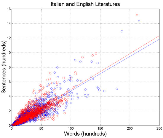
Figure 1. Scatterplot of sentences n_S versus words n_W. Italian Literature: blue circles and blue regression line; English Literature: red circles and red regression line. Samples refer to the averages found in the chapters: 1260 in Italian Literature, 1114 in English Literature; total: 2374. The blue and red lines are the regression lines with slope and correlation coefficients reported in Table 1.

Table 1. Slope m and correlation coefficient r. of $n_S$ versus $n_W$ of the regression lines drawn in Figure 1.

	m	$$\mathit{r}$$
Italian	0.0474	0.877
English	0.0493	0.819

2.2. Interpunctions versus Sentences

Figure 2 shows the scatterplot of interpunctions, $n_I$, versus sentences, $n_S$, for the Italian and the English literature. Table 2 reports slopes and correlation coefficients of the two regression lines drawn in Figure 2. The two literary corpora almost coincide—as far as the slope is concerned—as if the samples were extracted from the same database. This issue will be further discussed by considering the theory of linguistic channels in Section 3.

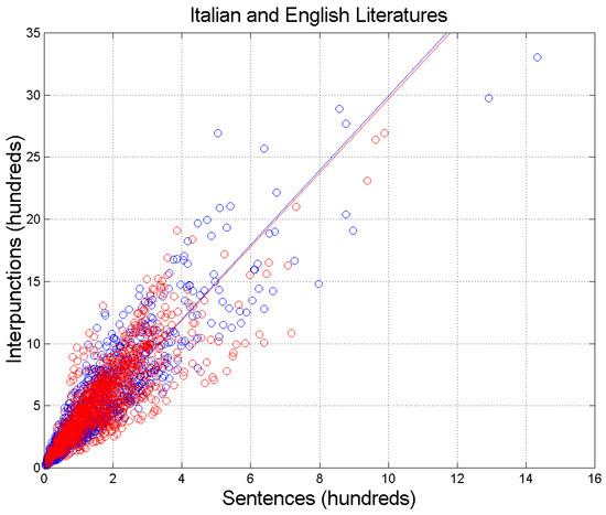
Figure 2. Scatterplot of interpunctions $n_I$ versus sentences $n_S$. Italian Literature: blue circles and blue regression line; English Literature: red circles and red regression line. The blue and red lines are the regression lines with slope and correlation coefficients reported in Table 2.

Table 2. Slope $m$ and correlation coefficient $r$ of interpunctions per chapter, $n_I$, versus sentences per chapter, $n_S$, of the regression lines drawn in Figure 2.

	$$\mathit{m}$$	$$\mathit{r}$$
Italian	2.994	0.913
English	2.969	0.853

2.3. Words per Sentence versus Word Interval per Sentence

Figure 3 shows the scatterplot of words per sentence, $P_F$, versus word intervals per sentence, $M_F$. It is interesting to notice a tight, similar linear relationship in both literatures; see slopes and correlation coefficients in Table 3. This issue will be further discussed by considering the theory of linguistic channels in Section 3.

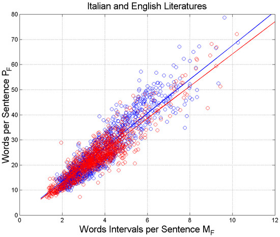
Figure 3. Scatterplot of $P_F$ versus $M_F$. Italian Literature: blue circles and blue regression line; English Literature: red circles and red regression line. The blue and red lines are the regression lines with slope and correlation coefficients reported in Table 3.

Table 3. Slope $m$ and correlation coefficient $r$ of $P_F$ versus $M_F$ of the regression lines drawn in Figure 3.

	$$\mathit{m}$$	$$\mathit{r}$$
Italian	6.763	0.937
English	6.421	0.914

The linear relationship shown in Figure 3 states that as a sentence gets longer, writers introduce more $I_P’\mathrm{s}$, regardless of the length of $I_P$. This seems to be a different mechanism—compared to that concerning the words that build-up $I_P$—that writers use to convey the full meaning of a sentence. We think that $M_F$ describes another STM processing beyond that described by $I_P$ and uncorrelated with it, as it can be deduced from the findings reported in the next sub-sections.

2.4. Word Intervals versus Words per Sentence

Figure 4 shows the scatterplot of the word interval, $I_P$, versus the words per sentence, $P_F$, for the Italian Literature (blue circles) and the English Literature (red circles). The magenta lines refer to Miller’s $7\pm 2$ law range (95% of samples). The black curve models the best fit relating $I_P$ to $P_F$ for all samples shown in Figure 4, as done in [1,2], given by:

$${\mathit{I}}_{\mathit{P}}=\left({\mathit{I}}_{\mathit{P}\mathit{\infty }}-\mathbf{1}\right)\times \left\{\mathbf{1}-{\mathit{e}}^{-\frac{\left({\mathit{P}}_{\mathit{F}}-\mathbf{1}\right)}{\left({\mathit{P}}_{\mathit{F}\mathit{o}}-\mathbf{1}\right)}}\right\}+\mathbf{1}$$

(6)

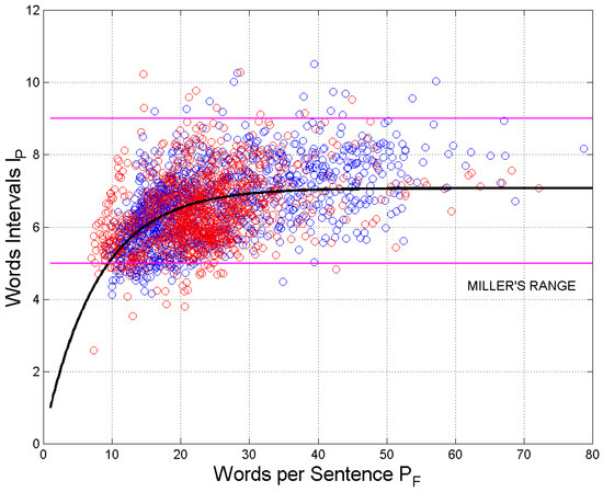
Figure 4. Scatterplot of $I_P$ versus $P_F$. Italian Literature: blue circles; English Literature: red circles. The black curve is given by Equation (6), and it is the best-fit curve for all samples. The magenta lines refer to Miller’s $7\pm 2$ law range of STM capacity.

As discussed in [1,2,3,4] and recalled above, Equation (6) models the saturation of $I_p$ as $P_F$ increases. Italian and English texts show no significant differences, therefore underlining a general behavior of human readers/writers independent of language.

In Equation (6), $I_{p\infty }=7.08$ and $P_{Fo}=7.88$. It is striking to notice that Miller’s range—which, as recalled, refers to 95% of samples—contains about 95% of all samples of $I_P$ shown in the ordinate scale of Figure 4 (precisely in the range from 4.8 to 8.6; see Section 2.6 below) and that the horizontal asymptote ($I_{p\infty }=7.08$) is just Miller’s range center value.

Defined the error $\epsilon =I_p-I_{P,model}$, between the experimental datum and that given by Equation (6), the average error is $-0.067$ for Italian and $0.063$ for English, with standard deviations of $0.852$ and $0.956$, respectively. Therefore, the two literary corpora are very similarly scattered around the black curve given by Equation (6).

In conclusion, the two literary corpora, for the purpose of the present study, can be merged together, and the findings obtained reinforce the conjecture that $I_P$ does describe the STM capacity defined by Millers’ Law.

2.5. Word Intervals per Sentence versus Word Intervals

Figure 5 shows the scatterplot of word intervals per sentence, $M_F$, versus word intervals, $I_P$. The correlation coefficient is $r=0.248$ in the Italian Literature and $r=-0.035$ in the English Literature, values which practically state that the two linguistic variables are uncorrelated. Similar values are also found for log values. The decorrelation between $M_F$ and $I_P$ strongly suggests the presence of two processing units acting independently of one another because zero correlation in Gaussian processes also means independence, a model we discuss further in Section 5.

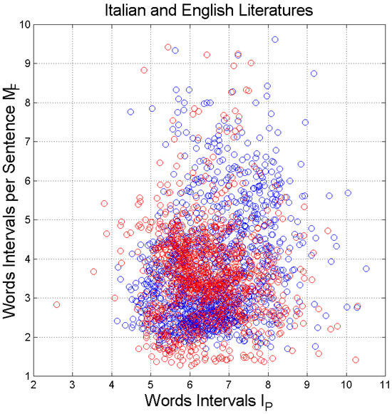
Figure 5. Scatterplot of $M_F$ versus $I_P$. Italian Literature: blue circles; English Literature: red circles. The correlation coefficient $r=0.248$ for Italian and $r=-0.035$ for English.

In the next sub-section, dealing with linguistic communication channels, we reinforce the fact that the two literary corpora can be merged together; therefore, they can give a homogeneous database of alphabetical texts sharing a common surface mathematical structure from which two STM processing units can be modeled.

2.6. Probability Distributions

In the previous sub-sections, we have noticed that there are no significant differences between the statistical features of Italian and English novels. Therefore, we are allowed to merge the two literary corpora for estimating the probability distributions of the deep-language variables. These are shown in Figure 6, Figure 7 and Figure 8, respectively, for $I_P$, $P_F$ and $M_F$. These probability distributions can be modeled with a three-parameter log-normal probability density function, as done for Italian Literature for $I_P$ in Reference [1], given by the general expression (natural logs):

$$f\left(x\right)=\frac{1}{\sqrt{2\pi }{\sigma }_x\left(x-1\right)}exp\left\{-\frac{1}{2}{\left[\frac{ln\left(x-1)-{\mu }_x\right)}{{\sigma }_x}\right]}^2\right\}\hspace{1em}\hspace{1em}x\ge 1$$

(7)

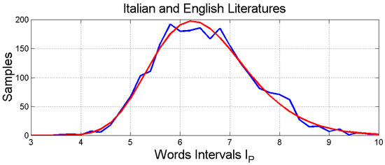
Figure 6. Histogram and log-normal probability modelling of $I_P$.

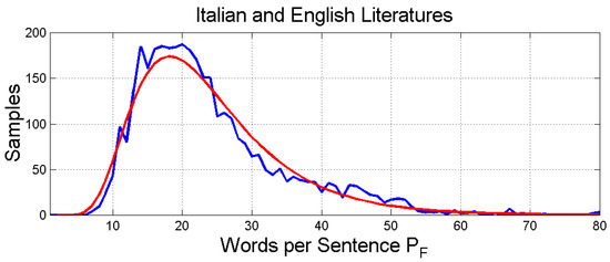
Figure 7. Histogram and log-normal probability modeling of $P_F$.

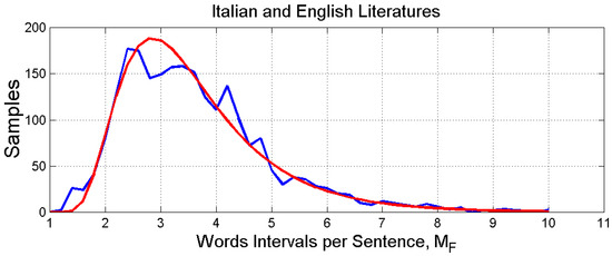
Figure 8. Histogram and log-normal probability modeling of ${ M}_F$.

In Equation (7), ${\mu }_x$ and ${\sigma }_x$ are, respectively, the average value and standard deviation. These constants are obtained as follows. Given the linear average value $m_x$ and the linear standard deviation $s_x$ of the random variable $x$, the standard deviation ${\sigma }_x$ and the average value ${\mu }_x$ of a three-parameter log-normal probability density function, defined for $x\ge 1$, are given by [34]:

$${\sigma }_x^2=ln\left[{\left(\frac{s_x}{m_x-1}\right)}^2+1\right]$$

(8)

$${\mu }_x=ln\left[\left(m_x-1\right)-\frac{{\sigma }_x^2}{2}\right]$$

(9)

Table 4 reports these values for the indicated parameters and the error statistics between the number of experimental samples and that predicted by the log-normal model. Table 5 reports some important linear statistical values that we will use in the next section.

Table 4. Average value ${\mu }_x$ and standard deviation ${\sigma }_x$ of the indicated variables and the average value and standard deviation of the error defined as the difference between the number of experimental samples and that predicted by the log-normal model.

	$${\mathit{\mu }}_{\mathit{x}}$$	$${\mathit{\sigma }}_{\mathit{x}}$$	Average Error	Standard Deviation of Error
${\mathit{I}}_{\mathit{P}}$	$\mathbf{1.689}$	$\mathbf{0.180}$	0.002	56.92
$P_F$	$3.038$	$\mathbf{0.441}$	0.049	12.44
$M_F$	$0.849$	$\mathbf{0.483}$	0.126	12.72

Table 5. Linear mean, standard deviation, and 95% probability range (Miller’s range) of the indicated variables.

	Mean	Standard Deviation	Miller’s Range (95%)
${\mathit{I}}_{\mathit{P}}$	$\mathbf{6.50}$	$\mathbf{1.00}$	$\mathbf{4.80}\mathbf{~}\mathbf{8.60}$
$P_F$	$23.98$	$\mathbf{10.64}$	$\mathbf{21.00}\mathbf{~}\mathbf{51.00}$
$M_F$	$3.63$	$\mathbf{1.36}$	$\mathbf{1.72}\mathbf{~}\mathbf{7.12}$

3. Linguistic Communication Channels in Texts

To study the chaotic data that emerge in any language, the theory developed in Reference [2] compares a text (the reference, or input text, written in a language) to another text (output text, “cross–channel”, written in any language) or to itself (“self-channel”), with a complex communication channel—made of several parallel single channels, two of which were explicitly considered in [2,4,5,7]—in which both input and output are affected by “noise”, i.e., by diverse scattering of the data around a mean linear relationship, namely a regression line, as those shown in Figure 1, Figure 2 and Figure 3 above.

In Reference [3], we have applied the theory of linguistic channels to show how an author shapes a character speaking to diverse audiences by diversifying and adjusting (“fine tuning”) two important linguistic communication channels, namely the Sentences channel (S-channel) and the Interpunctions channel (I-channel). The S-channel links $n_S$ of the output text to $n_S$ of the input text for the same number of words. The I-channel links $M_F$ (i.e., the number of $I_P’\mathrm{s}$) of the output text to $M_F$ of the input text for the same number of sentences.

In Reference [5], we have further developed the theory of linguistic channels by applying it to Charles Dickens’ novels and to other novels of English Literature (the same literary corpus considered in the present paper) and found, for example, that this author was very likely affected by King James’ New Testament.

In S–channels, the number of sentences of two texts is compared for the same number of words; therefore, they describe how many sentences the writer of text $j$ (output) uses to convey a meaning, compared to the writer of text $k$ (input)—who may convey, of course, a diverse meaning—by using the same number of words. Simply stated, it is about how a writer shapes his/her style for communicating the full meaning of a sentence with a given number of words available; therefore, it is more linked to the author’s style. These channels are those described by the scatterplots and regression lines—shown in Figure 1—in which we get rid of the independent variable $n_W$.

In I-channels, the number of word intervals $I_P$ of two texts is compared for the same number of sentences; therefore, they describe how many short texts make a full sentence. Since $I_P$ is connected to the STM capacity (Miller’s Law) and $M_F$ is linked—in our present conjecture—to the E-STM, the I-channels are more related to how the human mind processes information than to the authors’ style. These channels are those described by the scatterplots and regression lines—shown in Figure 2—in which we get rid of the independent variable $n_S$.

In the present paper, for the first time, we consider linguistic channels which compare $P_F$ of two texts for the same number of $M_F$; therefore, these channels are connected with the E-STM, as they are a kind of “inverse” channel of the I-channels. These channels are those described by the scatterplots and regression lines—shown in Figure 3—in which we get rid of the independent variable $M_F$. We refer to these channels as the $P_F$-channels.

Recall that regression lines, however, consider and describe only one aspect of the linear relationship, namely that concerning (conditional) mean values. They do not consider the scattering of data, which may not be similar when two regression lines almost coincide, as Figure 1, Figure 2 and Figure 3 show. The theory of linguistic channels, on the contrary, by considering both slopes and correlation coefficients, provides a reliable tool to compare two sets of data fully, and it can be applied to any discipline in which regression lines are found.

To apply the theory of linguistic channels [2,3], we need the slope $m$ and the correlation coefficient $r$ of the regression line between (a) $n_S$ and $n_W$ to study the S–channels (Figure 1); (b) $n_I$ and $n_S$ to study the I-channels (Figure 2); (c) $P_F$ and $M_F$ to study $P_F$—channels (Figure 3), values listed in Table 1, Table 2 and Table 3.

In synthesis, the theory calculates the slope $m_{jk}$ and the correlation coefficient $r_{jk}$ of the regression line between the same linguistic parameters by linking the input k (independent variable) to the output j (dependent variable) of the virtual scatterplot in the three linguistic channels mentioned above.

The similarity of the two data sets (regression lines and correlation coefficients) are synthetically measured by the theoretical signal-to-noise ratio ${\mathsf{\Gamma }}_{th}$ (dB) [2]. First, the noise-to-signal ratio $R$, in linear units, is calculated from:

$$R={(m_{jk}-1)}^2+\frac{1-r_{jk}^2}{r_{jk}^2}{m}_{jk}^2$$

(10)

Secondly, from Equation (7), the total signal-to-noise ratio is given (in dB) by:

$${\mathsf{\Gamma }}_{th}\left(\mathrm{d}\mathrm{B}\right)=-10\times {\mathrm{l}\mathrm{o}\mathrm{g}}_{10}R$$

(11)

Notice that when a text is compared to itself ${\mathsf{\Gamma }}_{th}=\infty$, because $r=1$, $m=1$.

Table 6 shows the results when Italian is the input language $k$ and English is the output language $j$; Table 7 shows the results when English is the input language $k$ and Italian is the output language $j$.

Table 6. Slope $m_{jk}$ and correlation coefficient $r_{jk}$ of the regression line between the same linguistic parameter of the two languages and the signal-to-noise ratio ${\mathsf{\Gamma }}_{th}$ (dB) in the linguistic channel. Input channel: Italian; output channel: English.

		$${\mathit{m}}_{\mathit{j}\mathit{k}}$$	$${\mathit{r}}_{\mathit{j}\mathit{k}}$$	$${\mathsf{\Gamma }}_{\mathit{t}\mathit{h}}$$
S-channel	$n_{S,Eng}$ versus $n_{S,Ita}$	1.040	0.994	18.37
I-channel	$n_{I,Eng}$ versus $n_{I,Ita}$	0.992	0.992	17.80
E-channel	$P_{F,Eng}$versus $P_{F,Ita}$	0.949	0.998	22.18

Table 7. Slope $m_{jk}$ and correlation coefficient $r_{jk}$ of the regression line between the same linguistic parameter of the two languages and the signal-to-noise ratio ${\mathsf{\Gamma }}_{th}$ (dB) in the linguistic channel. Input channel: English; output channel: Italian.

		$${\mathit{m}}_{\mathit{j}\mathit{k}}$$	$${\mathit{r}}_{\mathit{j}\mathit{k}}$$	$${\mathsf{\Gamma }}_{\mathit{t}\mathit{h}}$$
S-channel	$n_{S,Ita}$ versus $n_{S,Eng}$	0.962	0.994	19.01
I-channel	$n_{I,Ita}$ versus $n_{I,Eng}$	1.009	0.992	17.65
E-channel	$P_{F,Ita}$versus $P_{F,Eng}$	1.053	0.998	21.46

From Table 6 and Table 7, we can observe the following:

(a)

The slopes are very close to unity, implying, therefore, that the two languages are very similar in average values (i.e., the regression line).

(b)

The correlation coefficients are very close to 1, implying, therefore, that data scattering is very small.

(c)

The remarks in (a) and (b) are synthesized by ${\mathsf{\Gamma }}_{th}$ which is always significantly large. Its values are in the range of reliable results (see the discussion in References [2,3,4,5,6,7]).

(d)

The slight asymmetry of the two channels, Italian $\to$ English (Table 6) and English $\to$ Italian (Table 7), is typical of linguistic channels [2,3,4,5,6,7].

In other words, the “fine tuning” done through the three linguistic channels strongly reinforces the conclusion that the two literary corpora are “extracted” from the same data set, from the same “book”, whose “text” is interweaved in a universal surface mathematical structure that human mind imposes to alphabetical languages. The next section further reinforces this conclusion when text readability is considered.

4. Relationships with a Universal Readability Index

In Reference [6], we have proposed a universal readability index that includes the STM capacity, modeled by $I_P$, applicable to any alphabetical language, given by:

$$G_U=G-6\left(I_P-6\right)$$

(12)

With

$$G=89-10k{C}_P+300/P_F$$

(13)

$$k=<C_{P,ITA}>/<C_P>$$

(14)

In Equation (12), the E-STM is also indirectly present with the variable $P_F$ of Equation (13). Notice that text readability increases (text more readable) as $G_U$ increases.

The observation that differences between the readability indices give more insight than absolute values has justified the development of Equation (12).

By using Equations (13) and (14), the average value ${<10\times kC}_P>$ of any language is forced to be equal to that found in Italian, namely $10\times 4.48$. In doing so, if it is of interest, $G_U$ can be linked to the number of years of schooling in Italy [1,6].

There are two arguments in favor of Equation (14); the first is that $C_p$ affects a readability formula much less than $P_F$ [1]. The second is that $C_P$ is a parameter typical of a language which, if not scaled, would bias $G_U$ without really quantifying the change in reading difficulty of readers who are accustomed to reading shorter or longer words in their language, on average, than those found in Italian. This scaling, therefore, avoids changing $G_U$ only because in a language, on average, words are shorter or longer than in Italian.

Figure 9 shows the histogram of $G_U$. The mean value is $55.0$, the standard deviation is $11.0,$ and the 95% range is $35.0~78.5$.

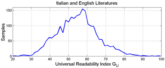
Figure 9. Histogram of $G_U$. The mean value is $55.0$, the standard deviation is $11.0,$ and the 95% range is $35.0~78.5$.

Figure 10 shows the scatterplot of $G_U$ versus $I_P$ in the Italian and English Literature. There are no significant differences between the two languages; therefore, we can merge all samples. The vertical black lines are drawn at the mean value $I_P=6.50,$ and at the values exceeded with probability $0.025$ ($I_P=4.8)$ and $0.975$ ($I_p=8.6).$ The range $4.8~8.6$ includes, therefore, 95% of the samples, and it corresponds to Miller’s range (Table 5).

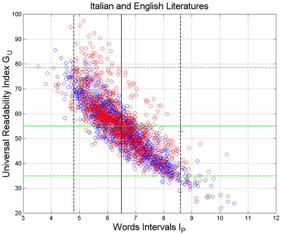
Figure 10. Scatterplot of the universal readability index $G_U$ versus the word interval $I_P$. Italian Literature: blue circles; English Literature: red circles. The vertical black lines are drawn at the mean value $I_P=6.5,$ and at the values $I_P$ is exceeded with a probability of 0.025 ($I_P=4.8)$ and 0.975 ($I_p=8.6).$ The range $4.8~8.6$ includes 95% of the samples, corresponding to Miller’s range $7\pm 2$. The horizontal green lines refer to $G_U$ (95% range $35.0~78.5$).

Figure 11 shows the scatterplot of $G_U$ versus $P_F$. The vertical black lines are drawn at the mean value $P_F=24.0,$ and at the values exceeded with probability $0.025$ ($P_F=11.0)$ and $0.975$ ($P_F=51.0).$ The range $11.0~51.0$ includes 95% of the merged samples corresponding to Miller’s range (Table 5). The horizontal green lines refer to $G_U$ (95% range $35.0~78.5$).

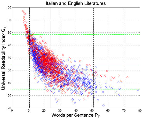
Figure 11. Scatterplot of the universal readability index $G_U$ versus the words per sentence s $P_F$. Italian Literature: blue circles and blue regression line; English Literature: red circles and red regression line. The vertical black lines are drawn at the mean value $P_F=24.0,$ and at the values exceeded with probability $0.025$ ($P_F=11.0)$ and $0.975$ ($P_F=51.0).$ The range $11.0~51.0$ includes 95% of the samples; therefore, it corresponds to Miller’s range $7\pm 2$ of $I_P$. The horizontal green lines refer to $G_U$ (95% range $35.0~78.5$).

Figure 12 shows the scatterplot of $G_U$ versus $M_F$. The vertical black lines are drawn at the mean value $M_F=3.58,$ and at the values exceeded with probability $0.025$ ($M_F=1.72)$ and $0.975$ ($M_F=7.12).$ The range $1.72~7.12$ includes, therefore, 95% of the samples, and it corresponds to Miller’s range (Table 5). The horizontal green lines refer to $G_U$ (95% range $35.0~78.5$).

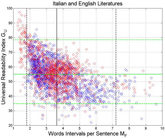
Figure 12. Scatterplot of the universal readability index $G_U$ versus the word intervals $M_F$. Italian Literature: blue circles and blue regression line; English Literature: red circles and red regression line. The vertical black lines are drawn at the mean value $M_F=3.58,$ and at the values exceeded with probability 0.025 ($M_F=1.72)$ and 0.975 ($M_F=7.12).$ The range $1.72~7.12$ includes 95% of the samples; therefore, it corresponds to Miller’s range. The horizontal green lines refer to $G_U$ (95% range $35.0~78.5$).

In all cases, we can observe that $G_U$, as expected, is inversely proportional to the deep-language variable involved in the STM processing. In other words, the larger the independent variable, the lower the readability index.

5. Two STM Processing Units in Series

From the findings reported in the previous sections, we are justified to conjecture that the STM elaborates information with two processing units, regardless of language, author, time, and audience. The model seems to be universally valid, at least according to how this largely unknown surface processing is seen through the lens of the most learned writings down several centuries. The main reasons to propose this conjecture are the following.

According to Figure 5, $M_F$ and $I_P$ are decorrelated. Moreover, because of log normality and correlation coefficients that are practically zero between log values, we can even say that the two variables are independent. This suggests the presence of two independent processing units working with different, although similar, “protocols”, the first capable of processing approximately $7\pm 2$ items (Miller’s Law)—capacity measured by $I_P$—and the second capable of processing $1~6$ items—capacity measured by $M_F$.

Figure 13 shows how these two capacities are related at equal probability exceeded. We can see that the relationship is approximately linear in the range $5~8$ of $I_P$ ($2~6$ of $M_F$).

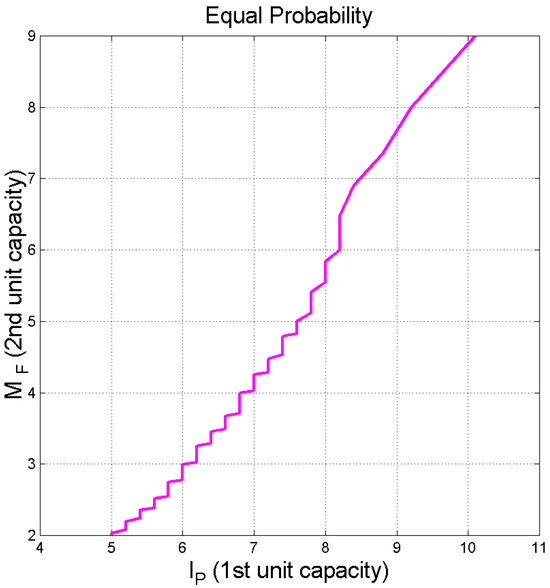
Figure 13. Capacity of the second STM processing unit, $M_F,$ versus the capacity of the first STM processing unit, $I_P,$ calculated at equal probability exceeded.

Figure 14 shows the ideal flowchart of the two STM units that process a sentence. After the previous sentence, a new sentence starts: The words $p_1$, $p_2$,…$p_j$ are stored in the first buffer, with the capacity given by a number approximately in Miller’s range, until an interpunction is introduced to fix the length of $I_P$. The word interval $I_P$ is then stored in the E-STM buffer up to $k=M_F$ items, from about 1 to 6, until the sentence ends. The two buffers are afterward cleared, and a new sentence can start.

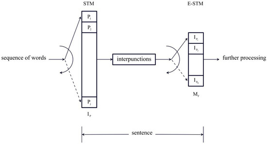
Figure 14. Flowchart of the two processing units that make a sentence. The words $p_1$, $p_2$,…$p_j$ are stored in the first buffer up to $j$ items, approximately in Miller’s range, until an interpunction is introduced to fix the length of $I_P$. The word interval $I_P$ is then stored in the E-STM buffer up to $k$ items, from about 1 to 6 items, until the sentence ends.

Let us calculate the overall capacity required by the full processing described in Figure 14. If we consider the 95% range in both processing units (Table 5), we get $4.80\times 1.72=8.26$ words and $8.60\times 7.12=61.23$ words.

We can roughly estimate the time necessary to complete the cycle of a sentence by converting the capacity expressed in words into a time interval required to read them by assuming a reading speed, such as 188 words for Italian or very similar values for other languages [9]. Notice, however, that this reading speed refers to a fast reading reader, not to a common reader of novels, whose pace can be slower, down to approximately 90 words per minute [35]. Reading 188 words in 1 min gives 2.6 and 19.5 s, respectively, values that become 5.3 and 30.1 s when reading 90 words per minute, which is very well contained in experimental findings concerning the STM processing [11,12,13,14,15,16,17,18,19,20,21,22,23,24,25,26,27,28,29,30,31].

6. Conclusions

We have shown that during a sentence, the alphabetical text is processed by the short-term memory (STM) with two independent processing units in series, with similar capacity. The clues for conjecturing this model has emerged by considering many novels belonging to the Italian and English Literatures.

We have shown that there are no significant mathematical/statistical differences between the two literary corpora by considering deep-language variables and linguistic communication channels. This finding underlines the fact that the mathematical surface structure of alphabetical languages—a creation of human mind—is very deeply rooted in humans, independently of the particular language used, therefore we have merged the two literary corpora in one data set and obtained universal results.

The first processing unit is linked to the number of words between two contiguous interpunctions, variable indicated by ${ I}_p$, approximately ranging in Miller’s $7\pm 2$ law range; the second unit is linked to the number of $I_p$’s contained in a sentence, variable indicated by $M_F$ and referred to as the extended STM, or E-STM, ranging approximately from 1 to 6.

We have recalled that a two-unit STM processing can be empirically justified according to how a human mind is thought to memorize “chunks” of information contained in a sentence. Although simple and related to the surface of language, the model seems to describe mathematically the input-output characteristics of a complex mental process, largely unknown.

The overall capacity required by the full processing of a sentence ranges from $8.3$ to $61.2$ words, values that can be converted into time by assuming a reading speed. This conversion gives the range $2.6~19.5$ s for a fast-reading reader and $5.3~30.1$ s for a common reader of novels, values well supported by experiments reported in the literature.

A sentence conveys meaning, therefore, the surface features we have found might be a starting point to arrive at the Information Theory that includes meaning.

Future work should be done on the readers of other literature of Western languages and on ancient readers of Greek and Latin Literature to assess whether their STM processing was, very likely, similar to that discussed in the present paper.

References

- Matricciani, E. Deep Language Statistics of Italian throughout Seven Centuries of Literature and Empirical Connections with Miller’s 7 ∓ 2 Law and Short–Term Memory. Open J. Stat. 2019, 9, 373–406. [Google Scholar] [CrossRef]
- Matricciani, E. A Statistical Theory of Language Translation Based on Communication Theory. Open J. Stat. 2020, 10, 936–997. [Google Scholar] [CrossRef]
- Matricciani, E. Linguistic Mathematical Relationships Saved or Lost in Translating Texts: Extension of the Statistical Theory of Translation and Its Application to the New Testament. Information 2022, 13, 20. [Google Scholar] [CrossRef]
- Matricciani, E. Multiple Communication Channels in Literary Texts. Open J. Stat. 2022, 12, 486–520. [Google Scholar] [CrossRef]
- Matricciani, E. Capacity of Linguistic Communication Channels in Literary Texts: Application to Charles Dickens’ Novels. Information 2023, 14, 68. [Google Scholar] [CrossRef]
- Matricciani, E. Readability Indices Do Not Say It All on a Text Readability. Analytics 2023, 2, 296–314. [Google Scholar] [CrossRef]
- Matricciani, E. Linguistic Communication Channels Reveal Connections between Texts: The New Testament and Greek Literature. Information 2023, 14, 405. [Google Scholar] [CrossRef]
- Matricciani, E. Short−Term Memory Capacity across Time and Language Estimated from Ancient and Modern Literary Texts. Study−Case: New Testament Translations. Open J. Stat. 2023, 13, 379–403. [Google Scholar] [CrossRef]
- Trauzettel−Klosinski, S.; Dietz, K. Standardized Assessment of Reading Performance:The New International Reading Speed Texts IreST. IOVS 2012, 53, 5452–5461. [Google Scholar]
- Miller, G.A. The Magical Number Seven, Plus or Minus Two. Some Limits on Our Capacity for Processing Information. Psychol. Rev. 1955, 63, 343–352. [Google Scholar]
- Atkinson, R.C.; Shiffrin, R.M. The Control of Short−Term Memory. Sci. Am. 1971, 225, 82–91. [Google Scholar] [CrossRef] [PubMed]
- Baddeley, A.D.; Thomson, N.; Buchanan, M. Word Length and the Structure of Short−Term Memory. J. Verbal Learn. Verbal Behav. 1975, 14, 575–589. [Google Scholar] [CrossRef]
- Mandler, G.; Shebo, B.J. Subitizing: An Analysis of Its Componenti Processes. J. Exp. Psychol. Gen. 1982, 111, 1–22. [Google Scholar] [CrossRef] [PubMed]
- Cowan, N. The magical number 4 in short−term memory: A reconsideration of mental storage capacity. Behav. Brain Sci. 2000, 24, 87–114. [Google Scholar] [CrossRef] [PubMed]
- Muter, P. The nature of forgetting from short−term memory. Behav. Brain Sci. 2000, 24, 134. [Google Scholar] [CrossRef]
- Grondin, S. A temporal account of the limited processing capacity. Behav. Brain Sci. 2000, 24, 122–123. [Google Scholar] [CrossRef]
- Pothos, E.M.; Joula, P. Linguistic structure and short−term memory. Behav. Brain Sci. 2000, 24, 138–139. [Google Scholar] [CrossRef]
- Bachelder, B.L. The Magical Number 4 = 7: Span Theory on Capacity Limitations. Behav. Brain Sci. 2001, 24, 116–117. [Google Scholar] [CrossRef]
- Conway, A.R.A.; Cowan, N.; Michael, F.; Bunting, M.F.; Therriaulta, D.J.; Minkoff, S.R.B. A latent variable analysis of working memory capacity, short−term memory capacity, processing speed, and general fluid intelligence. Intelligence 2002, 30, 163–183. [Google Scholar] [CrossRef]
- Saaty, T.L.; Ozdemir, M.S. Why the Magic Number Seven Plus or Minus Two. Math. Comput. Model. 2003, 38, 233–244. [Google Scholar] [CrossRef]
- Chen, Z.; Cowan, N. Chunk Limits and Length Limits in Immediate Recall: A Reconciliation. J. Exp. Psychol. Learn. Mem. Cogn. 2005, 3, 1235–1249. [Google Scholar] [CrossRef] [PubMed]
- Richardson, J.T.E. Measures of short−term memory: A historical review. Cortex 2007, 43, 635–650. [Google Scholar] [CrossRef] [PubMed]
- Jarvella, R.J. Syntactic Processing of Connected Speech. J. Verbal Learn. Verbal Behav. 1971, 10, 409–416. [Google Scholar] [CrossRef]
- Barrouillest, P.; Camos, V. As Time Goes By: Temporal Constraints in Working Memory. Curr. Dir. Psychol. Sci. 2012, 21, 413–419. [Google Scholar] [CrossRef]
- Mathy, F.; Feldman, J. What’s Magic about Magic Numbers? Chunking and Data Compression in Short−Term Memory. Cognition 2012, 122, 346–362. [Google Scholar] [CrossRef] [PubMed]
- Gignac, G.E. The Magical Numbers 7 and 4 Are Resistant to the Flynn Effect: No Evidence for Increases in Forward or Backward Recall across 85 Years of Data. Intelligence 2015, 48, 85–95. [Google Scholar] [CrossRef]
- Jones, G.; Macken, B. Questioning short−term memory and its measurements: Why digit span measures long−term associative learning. Cognition 2015, 144, 1–13. [Google Scholar] [CrossRef] [PubMed]
- Chekaf, M.; Cowan, N.; Mathy, F. Chunk formation in immediate memory and how it relates to data compression. Cognition 2016, 155, 96–107. [Google Scholar] [CrossRef]
- Norris, D. Short−Term Memory and Long−Term Memory Are Still Different. Psychol. Bull. 2017, 143, 992–1009. [Google Scholar] [CrossRef]
- Hayashi, K.; Takahashi, N. The Relationship between Phonological Short−Term Memory and Vocabulary Acquisition in Japanese Young Children. Open J. Mod. Linguist. 2020, 10, 132–160. [Google Scholar] [CrossRef]
- Islam, M.; Sarkar, A.; Hossain, M.; Ahmed, M.; Ferdous, A. Prediction of Attention and Short−Term Memory Loss by EEG Workload Estimation. J. Biosci. Med. 2023, 11, 304–318. [Google Scholar] [CrossRef]
- Rosenzweig, M.R.; Bennett, E.L.; Colombo, P.J.; Lee, D.W.; Serrano, P.A. Short−term, intermediate−term and Long−term memories. Behav. Brain Res. 1993, 57, 193–198. [Google Scholar] [CrossRef] [PubMed]
- Kaminski, J. Intermediate−Term Memory as a Bridge between Working and Long−Term Memory. J. Neurosci. 2017, 37, 5045–5047. [Google Scholar] [CrossRef] [PubMed][Green Version]
- Bury, K.V. Statistical Models in Applied Science; John Wiley: New York, NY, USA, 1975. [Google Scholar]
- Matricciani, E.; De Caro, L. Jesus Christ’s Speeches in Maria Valtorta’s Mystical Writings: Setting, Topics, Duration and Deep−Language Mathematical Analysis. J 2020, 3, 100–123. [Google Scholar] [CrossRef]
Disclaimer/Publisher’s Note: The statements, opinions and data contained in all publications are solely those of the individual author(s) and contributor(s) and not of MDPI and/or the editor(s). MDPI and/or the editor(s) disclaim responsibility for any injury to people or property resulting from any ideas, methods, instructions or products referred to in the content. |
© 2023 by the author. Licensee MDPI, Basel, Switzerland. This article is an open access article distributed under the terms and conditions of the Creative Commons Attribution (CC BY) license (https://creativecommons.org/licenses/by/4.0/).