Article

ABAC Policy Mining through Affiliation Networks and Biclique Analysis †

by
Abner Perez-Haro
*,‡ and
Arturo Diaz-Perez
Centro de Investigación y de Estudios Avanzados del Instituto Politécnico Nacional (Cinvestav), Department of Telecommunications, Guadalajara 45017, Mexico
*
Author to whom correspondence should be addressed.
This article is a revised and expanded version of a paper entitled Attribute-based access control rules supported by biclique patterns, which was presented at 2023 IEEE Ninth International Conference on Big Data Computing Service and Applications (BigDataService), Athens, Greece, 17–20 July 2023.
These authors contributed equally to this work.
Information 2024, 15(1), 45; https://doi.org/10.3390/info15010045
Submission received: 22 November 2023 / Revised: 31 December 2023 / Accepted: 8 January 2024 / Published: 12 January 2024
(This article belongs to the Special Issue Complex Network Analysis in Security)

Abstract

:
Policy mining is an automated procedure for generating access rules by means of mining patterns from single permissions, which are typically registered in access logs. Attribute-based access control (ABAC) is a model which allows security administrators to create a set of rules, known as the access control policy, to restrict access in information systems by means of logical expressions defined through the attribute–values of three types of entities: users, resources, and environmental conditions. The application of policy mining in large-scale systems oriented towards ABAC is a must because it is not workable to create rules by hand when the system requires the management of thousands of users and resources. In the literature on ABAC policy mining, current solutions follow a frequency-based strategy to extract rules; the problem with that approach is that selecting a high-frequency support leaves many resources without rules (especially those with few requesters), and a low support leads to the rule explosion of unreliable rules. Another challenge is the difficulty of collecting a set of test examples for correctness evaluation, since the classes of user–resource pairs available in logs are imbalanced. Moreover, alternative evaluation criteria for correctness, such as peculiarity and diversity, have not been explored for ABAC policy mining. To address these challenges, we propose the modeling of access logs as affiliation networks for applying network and biclique analysis techniques (1) to extract ABAC rules supported by graph patterns without a frequency threshold, (2) to generate synthetic examples for correctness evaluation, and (3) to create alternative evaluation measures to correctness. We discovered that the rules extracted through our strategy can cover more resources than the frequency-based strategy and perform this without rule explosion; moreover, our synthetics are useful for increasing the certainty level of correctness results. Finally, our alternative measures offer a wider evaluation profile for policy mining.

1. Introduction

Attribute-based access control (ABAC) is a relatively recent model for access control where rules are declared through attributes. The ABAC reference guide was launched by the National Institute of Standards and Technology (NIST) in 2014 [1]. The main characteristic of ABAC is its fine granularity, which allows a security administrator to create very specific rules; in contrast, writing detailed rules based on roles is a cumbersome task. Moreover, the current technological trends (e.g., Industry 4.0, smart homes, and smart cities [2,3,4]) make it necessary to define rules beyond roles. The ABAC rules are defined by combining the values of three types of attributes: user, resource, and session attributes.
Policy mining is an automated procedure for generating access rules by means of mining attribute–value patterns (a-v patterns, for short) from permissions of already exercised systems [5]. Since individual permissions are usually embedded in complex access mechanisms, the data to be mined are collected from access logs. Each log entry records useful information about the requester, the requested resource, and the environmental conditions.
Despite the benefits and the existing ABAC solutions in the market, ABAC requires meticulous planning, and establishing attribute-based rules from scratch is only workable in small scenarios, since it is imperative to analyze all the valid and invalid value combinations in the system [6]. Therefore, policy mining has been identified as the key for achieving widespread adoption of the attribute-based approach [7].
The policy mining approaches that offer convergence on large access logs (i.e., with thousand of users, resources and attribute–values, and even millions of entries), support the a-v patterns associated with rules through frequency [8,9,10]. Thus, a pattern is a good candidate for creating rules when its frequency in the log is greater than a frequency threshold. However, the problem with this strategy is that selecting a high support leaves many resources without rules (especially those with few requesters), and a low support leads to the rule explosion of unreliable rules. Therefore, the first challenge is to design an extraction algorithm that guarantees high coverage of the resources with a manageable number of rules.
A second challenge in ABAC policy mining is the difficulty of collecting examples for correctness evaluation. These examples are user–resource pairs which represent new access requests; examples labeled as permit are positive examples, and those labeled as deny are negative examples. The easiest way to obtain these pairs is to split the access log into training and test sets; however, positive pairs outnumber negatives in real access logs. To counteract class imbalance, it is possible to uniformly sample negative pairs from the set of pairs not registered in the log [11]; however, more sophisticated synthetics are required to confirm results or to reduce evaluation biases.
Due to the scarcity of negatives in access logs, alternative evaluation criteria to correctness are desirable. Two unexplored criteria for policy mining are peculiarity and diversity [12]. A pattern is peculiar when it is significantly different from other discovered patterns. A set of patterns is diverse if its elements differ significantly from each other. The advantage of peculiarity and diversity measures is that they do not depend on frequency and they do not need negative test examples to be computed. However, since the number of attribute–values can have the same order of magnitude as the number of users and resources in real access logs, many of the detected patterns can be discriminated as very peculiar, and the set of rules is very diverse. Therefore, a third challenge is the design of non-biased measures.
Our contribution is to model access logs as affiliation networks and to apply network and biclique analysis techniques in order to address the previously mentioned policy mining challenges. This new data representation is suitable (1) to extract ABAC rules supported by graph patterns without a frequency threshold, (2) to generate synthetic examples for correctness evaluation, and (3) to create alternative evaluation measures to correctness. We discovered that the rules extracted through our graph-based strategy can cover more resources than the frequency-based strategy and perform this without rule explosion; moreover, our synthetics are useful to increment the certainty level of correctness results; finally, our alternative measures offer a wider evaluation profile for policy mining.
Section 2 presents the background and preliminaries on ABAC, policy mining, its corresponding notation, and challenges. Section 3 describes the related work. Section 4 explains our graph-based proposal to solve three challenges of policy mining. Section 5 describes the datasets employed in our experiments. Section 6, Section 7 and Section 8 describe each of our solutions to the three identified challenges and present their corresponding experiments. Finally, Section 9 presents the conclusion and the future work.

2. Background and Preliminaries

2.1. Attribute-Based Access Control

We defined a notation for attribute-based access control (ABAC) rules similar to that proposed in [13]. In our notation, we integrated the main components of ABAC described in the NIST’s guide abacnist. Let U be the set of all users, R be the set of all resources, A u be the set of user attributes, and  A r be the set of resource attributes. We do not consider session attributes in this research.
Definition 1
(Attribute–value functions). Given a user u U and an attribute a u A u , the function f a u ( u , a u ) returns the corresponding attribute–value of u in a u , where the range of values for a u is V a u . Similarly, f a r ( r , a r ) and V a r for resources.
Definition 2
(Attribute–value patterns). A user pattern p u is a set of user attribute–value tuples:
p u = a u , ν a u A u , ν V a u ,
where A u A u . We define a resource pattern p r similarly for resources. We abbreviate these patterns as a-v patterns.
A user u U satisfies a pattern p u , denoted by u p u , if  a u , ν p u , f a u ( u , a u ) = ν . The resource satisfaction, denoted by r p r , has a similar definition.
Definition 3
(Access rules and policy). The elementary ABAC rule is a 4-tuple ρ p u , p r , o p , d , where p u is the associated user a-v pattern, p r is the associated resource a-v pattern, o p O P is an operation, and  d permit , deny is the rule decision. A policy is a set of access rules denoted by π.
In our research, we only consider the decision permit for rules (such specific kinds of rules are known as positive rules), and we only consider the operation access. Let u , r be a request of user u U to resource r R ; the request satisfies a rule ρ (denoted by u , r ρ ) if u ρ . p u and r ρ . p r .
In case p r = , a rule can be defined by the 4-tuple ρ p u , R , o p , d , where ρ . R R is the set of resources that the rule protects. A request u , r satisfies ρ if u ρ . p u and r ρ . R .
Definition 4
(ABAC mechanism). An ABAC mechanism is a function f π : ( U × R ) p e r m i t , d e n y which resolves access requests according to the following criteria: let π be the associated policy of the mechanism, f π returns permit to a request u , r if and only if ρ π such that u , r ρ , and it returns deny otherwise.

2.2. Policy Mining

Policy mining is an automatic procedure to generate access rules from existing single permissions in information systems; typically, the list of permissions is collected from access logs because each entry in a log records useful information for mining, such as descriptors of requesters and requested resources.
Definition 5
(Access log). We represent an access log through a set L ( U × R ) and a function f L : L permit , deny ; each element of L is a pair u , r which represents a log entry (i.e., it means u requested r), and  f L ( u , r ) returns the corresponding access decision recorded in the log for entry u , r (i.e., it indicates whether the request u , r was granted or not in the exercised system).
Access log L comprises the subset of positive entries  L + and the subset of negative entries  L , where L = ( L + L ) and:
L + = u , r L f L ( u , r ) = permit ,
L = u , r L f L ( u , r ) = deny .
Note that our definition does not admit label ambiguities by not allowing to entries to have more than one label.
Considering this representation of access logs and the rule format of Definition 3, policy mining for ABAC consists of creating a set of rules π by discovering user and resource patterns (i.e., p u and p u ) in an access log. Although there is no standard framework for applying this procedure, mining can be summarized through four consecutive processing phases:
  • Pre-processing transforms the access log into a suitable data structure in order to mine access patterns. Moreover, it guarantees that data values are either categorical or ordinal and there are no missing values, and it filters relevant attributes.
  • Rule extraction runs an extraction algorithm over the input data structure to select relevant patterns for creating ABAC candidate rules.
  • Post-processing deletes redundant rules and it can optionally create additional rules which could not be extracted by the previous phase.
  • Evaluation and improvement evaluates the performance of the final policy, and it attempts to improve the policy by relaxing too strict rules and making more robust over-permissive rules.
Two conventional criteria to evaluate policies are coverage (also known as completeness) and correctness. Coverage measures the proportion of entries of an access log L that are taken into account by a policy π :
cvg L ( π ) = u , r L + ρ π u , r ρ / L + .
Observe that this coverage definition only considers positive entries, since we are working only with positive rules.
On the other hand, correctness evaluates the ability of a policy to grant authorized accesses and to deny unauthorized accesses. Let Q + and Q be two sets of user–resource pairs whose elements represent new access requests, where Q + is the set of positive test examples and Q is the set of negative test examples. After labeling the elements of Q + as permit and the elements of Q as deny and evaluating Q + and Q through the ABAC mechanism f π , applying the correctness criteria consists of counting the number of true positives (TPs), false negatives (FNs), true negatives (TNs), and false positives (FPs) to compute measures such as recall, precision, f-score, and accuracy of binary classification. It is worth mentioning that Q + and Q are typically created from some elements of L + and L , respectively.

2.3. Challenges of ABAC Policy Mining

In spite of the promising advantages of policy mining for ABAC, we have identified some important challenges in this research area, which have to be addressed before deploying a mining solution in real systems. Given an access log L, mining procedures aimed for large-scale systems (i.e., with thousands of users, resources, and attribute–values and even millions of requests) model the input data as a set of transactions, where the elements of each transaction are attribute–values which correspond to the content of certain entry in L; then, a pattern discovery algorithm is run based on frequent itemsets to extract attribute–value patterns in order to create ABAC rules. The problem with such a strategy is that a frequency support has to be specified so that the algorithm detects only those patterns whose frequency is greater than this threshold. On the one hand, employing a high support can leave many resources without rules (especially those which have few requesters), whereas applying a low threshold leads to an explosion of unreliable rules.
Another challenge is the difficulty of having a set of examples to evaluate the correctness of policies, especially that of negative examples. The simplest procedure to obtain a test set is to set aside a subset of entries from the input access log for evaluation. However, it is common in real-world access logs that positive entries outnumber negative ones so that the latter represent less than 10 % of the log; this class imbalance can lead to biased correctness results. Moreover, it is also possible that many negative entries are not useful because their corresponding requests could be denied in specific environmental conditions that are not described in the log. On the other hand, constructing the test set of positive examples is also part of this challenge. Splitting the set of positive entries into training and test sets (e.g, an 80–20 split) is not possible for most of the resources, since most resources in real access logs have few requesters. For this reason, some policy mining solutions only evaluate rules for the most requested resources [10,11]. Additionally, this splitting can be counterproductive for a rule extraction strategy that takes into account the relationships among users and resources because deleting user–resource pairs can vanish the structures intended to be detected through that strategy.
Many studies on quality measures for data mining have been published in the last two decades [12]; the list of measures includes alternative measures that do not consider negative examples such as those based on peculiarity and diversity criterion. These measures can be useful as a supplement of the correctness evaluation because access logs are typically imbalanced as we mentioned before; moreover, they can provide a wider performance profile of policies. Thus, the third challenge is to adapt those quality measures to the specific task of policy mining in order to not obtain quality-biased results.
To summarize, we identified three challenges in ABAC policy mining:
  • The support problem in frequency-based pattern extraction: a high support leaves many resources uncovered, and a low support leads to a rule explosion.
  • The scarcity of negative examples to evaluate correctness of policies and even of positive examples when splitting is not possible due to the rule extraction technique.
  • Adapting alternative quality measures of data mining to the specific task of policy mining in order to not obtain quality-biased results.

3. Related Work

3.1. ABAC Rule Extraction

The rule extraction procedures of the state-of-the-art model access logs as a set of transactions and apply different predictive and descriptive techniques of data mining such as those in [14,15]. Predictive methods induce models or theories from labeled examples. The resulting models are employed to predict labels of new examples. The work of Xu et al., which is considered to be the first work on ABAC rule mining in the literature, falls into this category [13]; they used a technique similar to inductive logic programming that learns rules from facts. This approach generalizes seed permissions through a merging procedure to create rules. Medvet et al. employed an evolutionary algorithm with a divide-and-conquer strategy, which generates a new rule in every iteration [16]. Iyer et al. proposed a heuristic approach based on the PRISM algorithm [17]; they were the first to explore the extraction of negative authorization rules. The disadvantage of predictive methods is that they require non-sparse logs and labeled entries. In addition, [8] points out that these methods do not offer convergence on large datasets. Some authors have employed non-symbolic classifiers such as support vector machines (SVMs) [11] and neural networks [18] for mining large datasets, but they are difficult to train when categorical values of logs are anonymized and granted entries outnumber the denied ones.
Descriptive methods detect regular patterns in the data using the unsupervised approach. They have the advantage of not needing labeled entries to detect rules. The evidence of patterns is based on their frequency, and the frequency thresholds are defined by a user. Jabal et al. [9], Cotrini et al. [10], and Karimi et al. [8] employed these kinds of methods; in spite of their particularities, all coincide in using frequent itemsets as attribute–value patterns for their rules. Because only this strategy offers convergence on large datasets, we focused our research on the unsupervised approach.
Cotrini et al. presented the Rhapsody algorithm in [10], which is based on the subgroup discovery technique. Jabal et al. proposed a policy mining framework referred to as Polisma, which generates candidate rules through association rules [9], where rule antecedents are user patterns and rule consequents are resource patterns. Karimi et al. presented a clustering-based strategy in [8]. They reduced the search space of rules by grouping entries through a clustering algorithm and extracted rules from each cluster detecting the frequent attribute–values.

3.2. Correctness Evaluation

In order to deal with the class imbalance of access logs or to create ad hoc test examples, the solution is to generate synthetic user–resource pairs. Since such pairs are associated with attribute–value patterns, this generation procedure has to be intended for either categorical or ordinal variables. There is a great variety of techniques in the literature to generate synthetic categorical data; they fall into two categories: process-based techniques and data-based techniques. The former employ simulations that describe an underlying phenomenon, and the latter are trained on observed data; since in most cases phenomena are complex, the second techniques are preferred for data mining applications. Some data-based methods are as follows: Bayesian networks, categorical latent Gaussian processes, mixtures of product of multinomials, and generative adversarial networks [19]. However, since these methods are difficult to train or require large input datasets, they are not the best choice for policy mining.
A workable solution to generate synthetic test data for policy mining is to sample examples from the set of requests not present in the log access. For example, a straightforward procedure for creating synthetic negatives is to uniformly sample user–resource pairs [11]. However, in order to have more realistic examples, it is required to apply feature filters after sampling. For instance, Yanez-Sierra et al. proposed to filter pairs according to a vertex similarity function for network link prediction [20]; they argue that good positive examples are those pairs which exhibit a high similarity score between the requester and the requested element, whereas good negative examples are those which exhibit a low similarity score but one that is greater than zero. However, this solution was intended for evaluating access rules created from graph topological attributes instead of categorical attributes.
The problem statement of recommender systems is similar to the one of synthetic pair generation for policy mining. A recommender system suggests new items to users (i) based on the content of users and items, (ii) based on the ratings given by users, and (iii) based on the context of users and items [21,22]. However, one subtle difference between policy mining and the research area of recommender systems is that in the former, the number of new user–resource pairs per resource has to be proportional to the number of requesters of the resource, whereas in the latter it is desired to have as many recommended items per user as possible.

3.3. Alternative Evaluation Criteria to Correctness

Instead of just evaluating performance of policies and access rules through correctness, other evaluation criteria are available in the literature [12,23]. Such criteria are divided into two categories: objective, which is based on probability, statistics or information theory, and subjective, which takes into account the final user. The objective criteria are subdivided into the following categories:
  • Generality: A pattern is general if it covers a relatively large subset of a dataset. All access rule extraction solutions based on frequency support employ this criterion to select rule candidates.
  • Reliability: A pattern is reliable if the relationship described by a pattern occurs in a high percentage of applicable cases. In the case of association rules, the confidence measure falls into this category. Cotrini et al. adapted conventional confidence to measure reliability of ABAC rules [10].
  • Conciseness: A pattern is concise if it contains few attribute–value pairs. Molloy et al. defined a conciseness measure referred to as weighted structural complexity (WSC) for role-based access policies [24]. Xu et al. adapted this measure to ABAC. Other publications which employ a customized version of WSC are [8,25].
  • Peculiarity: A pattern is peculiar if it is far away from the other discovered patterns according to some dissimilarity measure.
  • Diversity: A set of patterns is diverse if its elements differ significantly from each other.
The most important characteristic of peculiarity and diversity is that they do not depend on the frequency of patterns; in contrast, they are proportional to the dissimilarity between a pattern and the rest of the patterns. As far as we are concerned, no previous works have presented peculiarity and diversity measures for policy mining. We describe some of these kinds of measures for generic applications. Zhong and Yao [26] proposed a peculiarity factor for tabular data. Yang et al. [27] extended this concept for density-based outlier detection with continuous variables by constraining the computation to pattern neighborhoods. Dong and Li [28] defined a peculiarity measure for association rules, known as neighborhood-based unexpectedness.
Hilderman and Hamilton [29] proposed the measurement of diversity by computing a statistical indicator (e.g., variance, entropy, Gini index) of the frequency distribution of attribute–value tuples; they argued that a set of tuples is diverse if the distribution is far from the uniform distribution. Huebner [30] explored diversity evaluation for the association rules employing the strategy of [29]. Graph summarization is another research area where diversity is employed to determine whether a summary is informative. For example, Zhang et al. [31] summarize graphs through graphs of vertex partitions, and such a graph is diverse if exhibits strong relationships between partitions with different attribute–values.

4. Our Proposal

We propose to model access logs as affiliation networks, analyze such networks, and process their biclique formations in order to achieve the following objectives:
  • Increase the policy coverage and deal with rule explosion.
  • Generate synthetic examples for correctness evaluation of rules.
  • Design alternative evaluation measures to correctness measures.
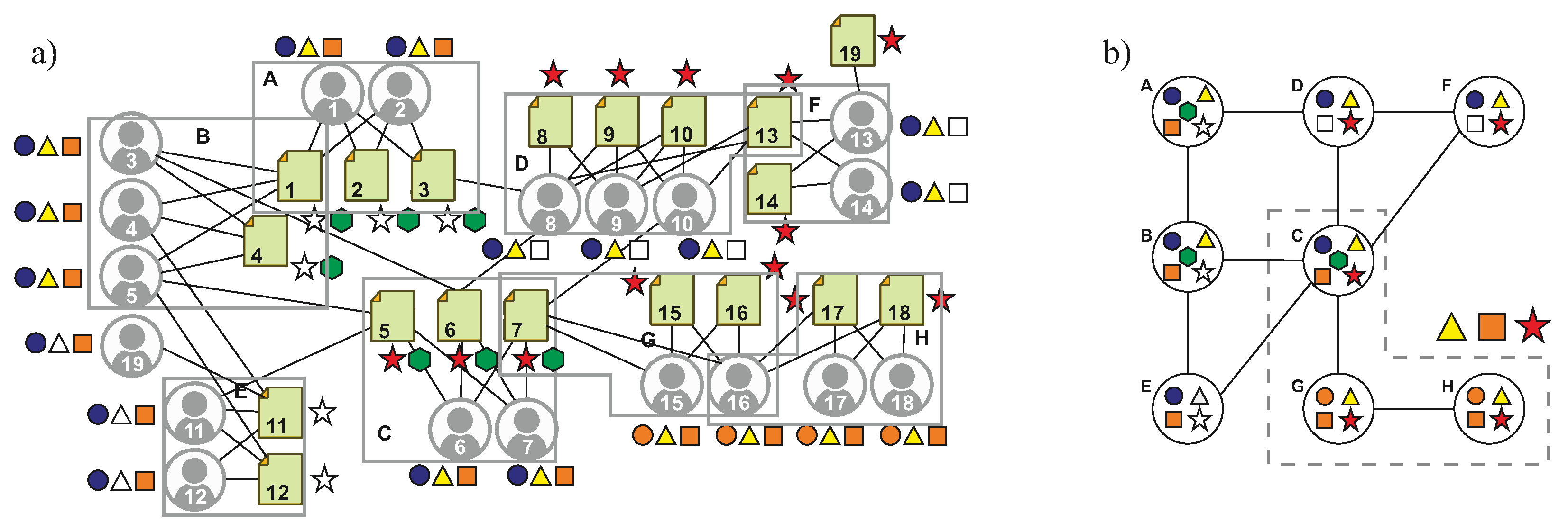
An affiliation network is a graph that consists of two sets of disjoint vertices, which are known as the top set and bottom set, and the edges between these sets of vertices. A biclique is a fully connected subgraph of an affiliation network. We model access logs through affiliation networks the following way:
Definition 6
(Access control graph (ACG)). Given an access log L, an access control graph G u r ( U , R , E ) is an affiliation network that represents L, where G u r . U U is the top set of vertices, G u r . R R is the bottom set of vertices and G u r . E ( G . U × G . R ) is the set of edges. There is an edge u , r G u r . E if and only if there exists an entry u , r in the log L + .
Notice that our definition only takes into account positive entries for creating an ACG because we only consider the extraction of positive access rules in this work. Additionally, we define two functions for such networks: (i) N ( v ) , which returns the set of adjacent vertices (known as neighbors) of vertex v ( G u r . U G u r . R ) , and (ii) function deg ( v ) , which returns the number of neighbors of v, which is known as the degree of v.
In a previous work [32], we observed that logs modeled through ACGs exhibit two important properties of complex networks [33], so it is possible to apply these network analysis techniques to discover useful access patterns for ABAC policy mining:
  • Small-world property: ACGs are structured in small fully connected subgraphs known as bicliques (which can be interpreted as collaboration groups of users through specific resources), and the average hop distance of ACGs is much shorter than the total vertices [34,35].
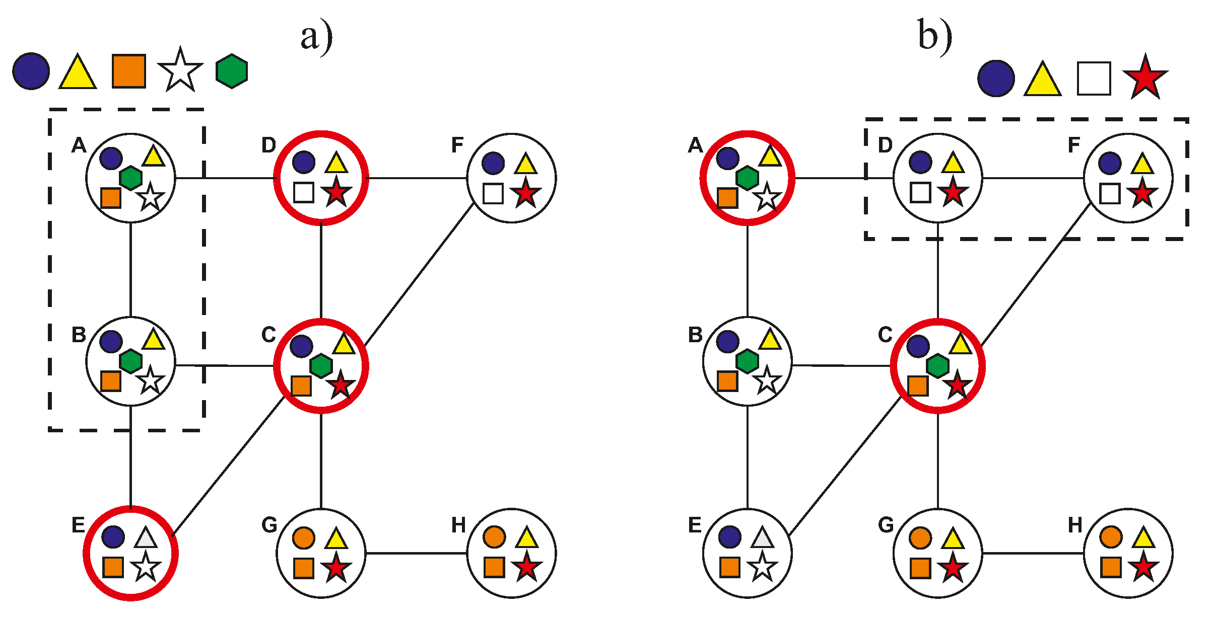
  • Homophily property: members of each biclique tend to share attribute–values, close bicliques are similar, and distant bicliques are dissimilar [36].
Figure 1a shows an example of a small access control graph, which has small-worldness and exhibits the homophily property. Observe that it has biclique formations, and users of biclique A share three attribute–values: the resources of A share one value, values of biclique A are similar to those of biclique B and D and values of biclique A are dissimilar to those of biclique H. We explain below the analysis techniques applied to the access control graph to achieve the stated objectives.

4.1. Our Solution for Objective 1

In order to increase the policy coverage and to deal with rule explosion, it is required to reformulate the attribute–value patterns associated with access rules and therefore to apply a different procedure to extract such patterns.
First, let K be the set of maximal bicliques of G u r , such that each element in K is a fully connected induced subgraph (i.e., biclique) denoted by κ ( U , R ) , where κ . U G u r . U and κ . R G u r . R . The term ‘maximal’ means that no biclique in K is a subgraph of another biclique in K; in this document, when we mention the term ‘bicliques’, we refer always to maximal bicliques. We also define the function f p u ( κ ) , which returns the longest pattern p u from biclique κ , such that the frequency of p u in κ . U is equal to κ . U (similarly, f p r ( κ ) for resources). From bicliques, we can define the following type of pattern:
Definition 7
(Biclique graph pattern (BGP))
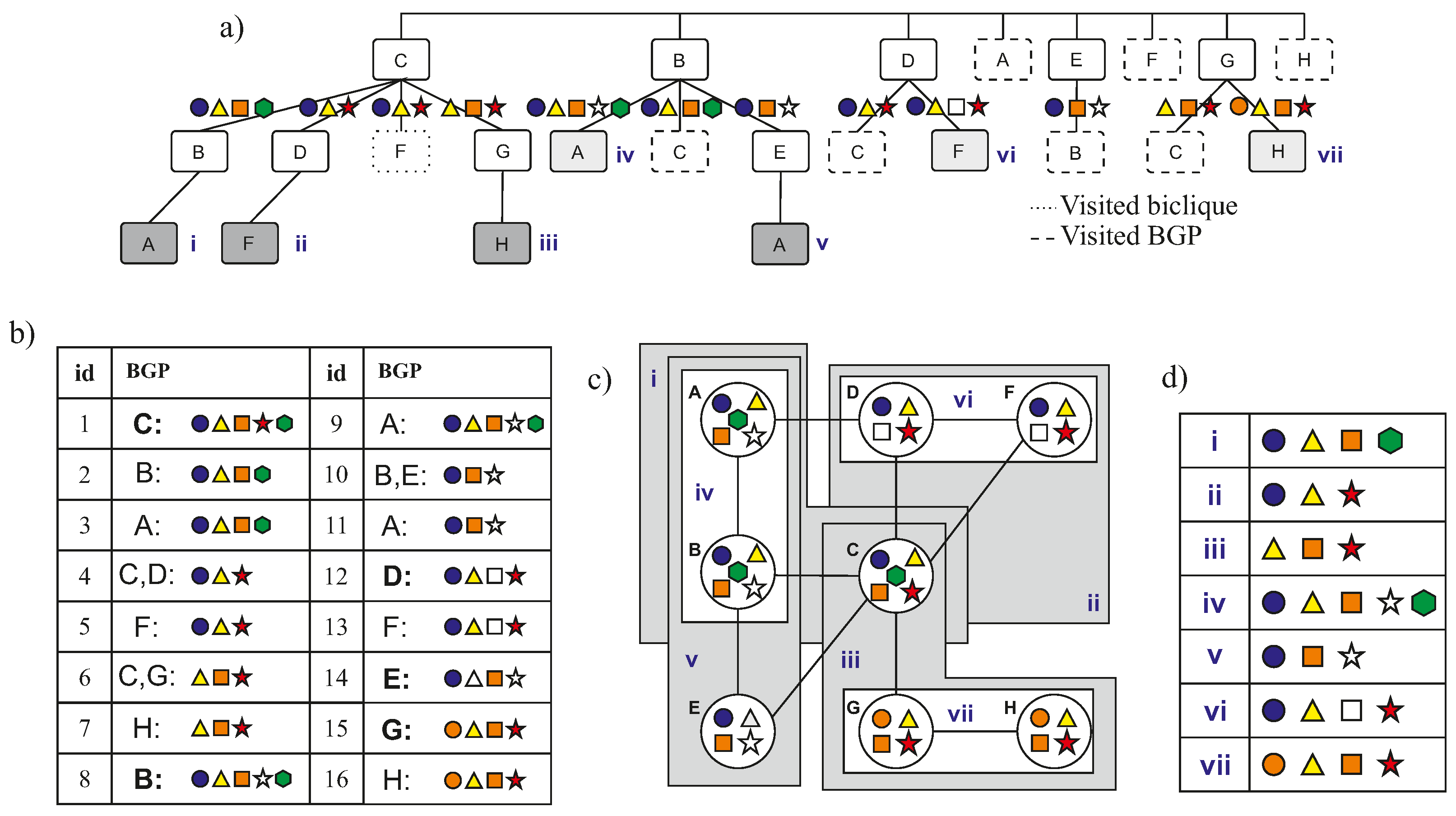
. A biclique graph pattern is a 3-tuple P ( K , p u , p r ) , where P . K is a subset of connected bicliques of G u r such that:
P . p u = κ P . K f p u ( κ ) ,
P . p r = κ P . K f p r ( κ ) ,
where f p u ( κ ) is the subset of user attribute–values shared by all users of biclique κ (similarly, f p r ( κ ) for resources).
For example, a biclique graph pattern in Figure 1a is P ( K , p u , p r ) such that P . K contains the connected bicliques C, G, and H; P . p u corresponds to triangle–yellow and square–orange and P . p r corresponds to star–red. Therefore, a candidate ABAC positive rule can be inferred which states that resources with star–red are authorized for users fulfilling triangle–yellow and square–orange.
In order to extract our patterns, it is required to modify the implementation of pre-processing and rule extraction phases of policy mining because conventional mining is based on frequent patterns (FPs). First, instead of directly extracting BGPs from the ACG, we transform this network into a suitable representation for our extraction algorithm:
Definition 8
(Graph of bicliques). The graph of bicliques of an access control graph G u r is a graph G κ ( K , E ) , where G κ . K K is its set of vertices which corresponds to a set of maximal bicliques of G u r , and  G κ . E ( G κ . K × G κ . K ) is its set of edges. An edge e = ( κ , κ ) G κ . E means the biclique κ and κ relate structurally to each other.
Figure 1b shows the resulting graph of bicliques of the ACG of Figure 1a, and the BGP P of our previous example. Secondly, we designed a bottom-up algorithm to detect BGPs starting from bicliques as building blocks, and agglomerating adjacent similar bicliques in a depth-first search fashion to create larger substructures. The procedure is summarized as follows:
For each biclique κ in the graph G κ :
  • For each combination p of at least l 1 attribute–values of κ :
    -
    Try to find at least other s 1 0 vertices in G κ such that they are connected to κ and share p to create a new biclique graph pattern P.
The resulting set of biclique graph patterns after applying our procedure is P s l (where s 1 and l 1 ), such that P P s l :
P . K s P . p u P . p r l ,
and corresponding ABAC rules are:
π = ρ i | P i P s l
ρ i P i . p u , P i . p r , access , permit .
For Objective 1 of our research, the resulting rules must achieve the following requirements:
  • High coverage: the set of rules must cover most of the log entries and many of the resources (especially those with few requesters).
  • Manageable rule explosion: the total number of rules must be much lower than the number of log entries.
For measuring the first requirement, we used the log coverage of Equation (4), and we defined the following measure:
Definition 9
(Resource coverage). The resource coverage of the rule set π in the resource subset R ¯ R (denoted by cvg R ( π , R ¯ ) ) is the ratio R π / R ¯ , where R π corresponds to the resources in R ¯ covered by π:
R π = r | r R ¯ ( ρ π , r ρ . p r ) .

4.2. Our Solution for Objective 2

In order to evaluate the correctness of ABAC policies, we propose a method to generate positive and negative synthetic examples (denoted by S = ( S + S ) ) by means of applying the ideas of content and context from recommender systems to our access control graph. Generating negative synthetics has the purpose of compensating for the lack of negative examples in access logs, and creating positive examples is desirable to avoid degrading biclique formations of access control graphs by splitting the set of positive entries into training and test sets (remember that integrity of bicliques is required in the rule extraction phase).
Given an access control graph G u r , the context distance of a pair u , r G u r . E is the minimum number of hops to reach u from r, and the content similarity of u , r is the proportion of attribute–values of u which are present in the neighbors of r. Thus, given a resource r G u r . R , our generation method for positives is to find users in G u r that are similar in context and content to r. On the other hand, for negatives, we employ the empirical evidence presented by Tang et al. in [37], which states that the geodesic distance between the end points of a not permitted pair u , r should be close to each other but not as the end points of possible permitted pairs. Therefore, generating negatives for r is to find users in G u r that are similar in context and content to r, but not as the positive examples.
For instance, in Figure 1a, a positive example for resource 4 is user 11, and a negative example for resource 4 is user 10. In contrast, the state-of-the-art uniform sampling strategy can suggest user 17 as a negative example for resource 4 (i.e., a very distant user). We will show in Section 7 that evaluating through our generation procedure is useful to increment the certainty level of correctness results.

4.3. Our Solution for Objective 3

As an alternative to correctness evaluation, we propose a peculiarity measure for ABAC rules and a diversity measure for ABAC policies that takes into account the relationships of attribute–value patterns in a network structure. Conventional peculiarity was proposed by Zhong et al. in [26], and it considers an attribute–value pattern as peculiar if differs significantly from the rest of the patterns. This conventional definition will discriminate most attribute–value patterns as peculiar in policy mining applied to large-scale access systems, since such systems can manage thousands of attribute–values and since this quantity is about the order of magnitude of the total users and resources in such scenarios.
In order to avoid this measurement bias, we propose a peculiarity measure where dissimilarity is computed with respect to a data neighborhood. The notion of a neighborhood is crucial for this task because a rule can be very peculiar with respect to the whole data but not necessarily with respect to its neighborhood. It is possible to define the neighborhood of an ABAC rule or an attribute–value by locating its corresponding biclique graph pattern in the graph of bicliques; for example, Figure 2 shows the neighboring data of two BGPs, which correspond to the adjacent bicliques of the patterns. As an example of how our proposal avoids biases, observe the attribute–value star–white in the BGP of Figure 2a, which is very peculiar in the pattern with respect to all the data; however, star–white is not very peculiar considering only the neighboring bicliques (i.e., bold red circles). In contrast, square–white is very peculiar for the pattern of Figure 2b with respect to all the data and their neighbors. Finally, we propose a diversity measure based on the distribution of our peculiarity measure because a very diverse policy is that whose rules are very peculiar.

5. Datasets

5.1. Reference Access Logs

In conducting our research, we employed two public access logs, which contain real requesting activity from Amazon Inc., and three synthetic access logs:
  • Amazon Kaggle (AZKAG): This dataset contains 32 K requests of 9 K users to 7 K resources. The dataset was provided by the Kaggle competition Employee Access Challenge in 2013 [38].
  • Amazon UCI (AZUCI): This dataset has 716 K entries which specify the time and date of requests. There are 36 K registered users in the system, of which 17 K have at least one request, and  6.4 K requested resources. It is available in the UCI Machine Learning Repository [39].
  • Xu and Stoller datasets: This is a collection of three synthetic datasets created by Xu and Stoller in [13]: University (UN), Healthcare (HC) and Project Management (PM). UN controls access to the resources of a university, HC controls access to electronic health records, and PM controls access to different data resources such as budgets, schedules, and tasks.
Table 1 shows the characteristics of these five datasets. Notice that most of the entries in the datasets are granted entries (see the third column), and the five datasets contain many infrequent attribute–values since the number of values is comparable to the number of users and resources of the logs (see the seventh column). Amazon’s datasets record the activity of thousands of users and resources, whereas the synthetic ones only offer support to hundreds of elements. Another important difference between real and synthetic access logs is the frequency distribution of their resources (see the last three columns); on one hand, in the real ones about 80 percent of the resources have few requesters, and the number of users of the resources with many requesters deviates substantially from the average. On the other hand, all resources in synthetic datasets have few requesters and are in the range from 1 to 10 users.

5.2. Access Control Graphs

We created the corresponding access control graphs (ACGs) of the reference access logs. We selected a list of relevant attributes from ( A u A r ) , and we ensured that the log entries of L were in categorical format before creating the ACGs. Afterwards, we characterized these networks through a clustering coefficient and a homophily degree measure.
The coefficient we employed is a local clustering coefficient defined in [40] for bipartite graphs:
C C l ( v ) = # closed two paths in v # two paths in v ,
where v is a vertex in ( G u r . U G u r . R ) , and the coefficient can be interpreted as either the probability that two requesters of resource ( v = r ) R have another resource r R in common or the probability that two resources requested by user ( v = u ) U have another requester u U in common. We defined the following homophily degree for bipartite graphs:
H = h s h s + h d ,
where h s is the number of wedges (i.e., number of two-paths) whose ends have at least one attribute–value in common, and  h d is the number of wedges whose ends have no attribute–values in common.
Table 2 shows the characteristics of the generated access control graphs. The five graphs are sparse, i.e.,  G u r . E G u r . U · G u r . R . They exhibit the small-world property because the average value of the local clustering coefficient is greater than the values of the corresponding random graph models, and the average path lengths satisfy L a v g ( G u r ) G u r . U G u r . R ; we created the models using the Molloy–Reed approach in [41], which keeps the size and the degree distribution of the original graphs. Moreover, they exhibit the homophily property since their homophily degree is considerably greater than zero. These interesting results reveal that it is possible to extract biclique graph patterns from either these reference datasets or any access log with similar characteristics.

6. Increasing Coverage and Dealing with Rule Explosion

6.1. Description of Our Solution

Our solution to increase coverage and to deal with rule explosion is to extract biclique graph patterns (BGPs) from access control graphs (ACGs). In order to achieve this objective:
  • Transform the input ACG into a graph of bicliques, which is a suitable data representation to extract BGPs;
  • Execute the extraction algorithm on the graph of bicliques, which is based on depth-first search.

6.1.1. Generating the Graph of Bicliques

The first step to create the graph of bicliques is to detect and process the bicliques of the input ACG following the procedure below.
  • Detecting bicliques in the ACG:
  • Enumerate the maximal bicliques of G u r to obtain the set K.
  • For all κ i K ( 1 i K ), find an a-v pattern p u ( i ) that is present in all the elements of κ i . U and an a-v pattern p r ( i ) that is present in all the elements of κ i . K . We computed these patterns by mining closed frequent itemsets from each single biclique with maximum support, and we kept the longest itemset. Finally, we created the mappings κ i ( f p u ( κ i ) = p u ( i ) ) and κ i ( f p r ( κ i ) = p r ( i ) ) .
  • Obtain the subset of exploitable bicliques K ¯ K such that κ K ¯ , f p u ( κ ) 1 (i.e., those bicliques having a non-empty user a-v pattern).
  • If there is an explosion of bicliques, apply Algorithm 1 over K ¯ to reduce the number of bicliques. This procedure is based on the greedy max k-cover algorithm, which selects the biclique that covers more remaining users and resources of K ¯ in each iteration.
The second step is to generate the graph of bicliques from the detected bicliques.
Algorithm 1 Obtain a reduced set of bicliques
1:
begin:  getReducedBCs ( K , U , R )
Input: K is a set of bicliques, and U and R are a set of considered users and resources, respectively.
Output:  K is the reduced set of bicliques.
2:
    Let K ^ K be the set of bicliques with at least one frequent attribute–value.
3:
    Let U ^ U be the set of users in K ^ .
4:
    Let R ^ R be the set of resources in K ^ .
/* Greedy algorithm for maximum coverage */
5:
     k 0.1 K ^
6:
     X U ^ R ^
7:
     S S κ K ^ , S = ( κ . U κ . R )
8:
    Init K as an empty set
9:
    for  i = 1 , , k  do
10:
        Let S i be one of the sets in S which maximizes S i X
11:
         X X S i
12:
         K . add ( κ i ) such that κ i K ^
13:
    end for
14:
    return  K ( K K ^ )
15:
end
  • Generating the graph of bicliques:
  • Compute the closeness matrix W for all κ , κ ( K ¯ × K ¯ ):
    W ( κ , κ ) = v κ . V v κ . V α v κ α v κ A ( v , v )
    α v κ = 1 α v v κ . V 1 O v v A ( v , v )
    α v = κ K ¯ v κ . V 1 O v v A ( v , v ) ,
    where κ . V = ( κ . U κ . R ) , and  O v v is the number of bicliques in K that share the edge v , v U × R . A is the adjacency matrix of the access control graph G u r , which is defined as:
    A ( v , v ) = 1 if v , v G u r . E 0 otherwise
  • Create the graph G κ ( K , E , w ) from W such that G κ . K = K ¯ , discarding the edges with weights that are too small.
  • In the case of obtaining a graph of bicliques too dense, apply the following procedure based on the work of [42]:
    (a)
    Let E x be the incident edges on κ x G κ . K . For all κ x , κ y E x and for all κ x G κ . K , compute the ranking function:
    rank x ( y ) = κ N ( κ x ) w > w + 1 ,
    such that w = G κ . w κ x , κ y , and  w = G κ . w κ x , κ .
    (b)
    Sort the elements of E x for all κ x G κ . K in descending order, according to rank x ( y ) .
    (c)
    Select the top deg ( κ u ) α elements of E x , for all κ x G κ . K , α 0 , 1 , and discard the rest of the edges.

6.1.2. The Extraction Algorithm

We designed a bottom-up algorithm to detect our patterns starting from bicliques as building blocks and agglomerating adjacent similar bicliques to create larger substructures. After obtaining the graph patterns and the corresponding rules, we reduced the total rules by clustering similar rules. Finally, we discarded graph patterns that were too small and with only frequent attribute–values because their topological support was negligible.
  • Description of the algorithm
Our extraction algorithm receives as input the graph of bicliques G κ , and it returns the set of graph patterns P s l and the corresponding rule set π . The first step is to select the parameters s and l, which specify the minimum number of groups and the minimum number of attribute–values for all graph patterns P P s l , respectively. The second step is to enumerate P s l by means of Algorithm 2, which traverses G κ in a depth-first search (DFS) fashion from each source vertex κ G κ . K sorted by maximum degree.
Algorithm 2 Detect graph patterns
1:
begin:  graphPatterns ( G κ , s , l )
2:
    Init P s l as an empty set
3:
     κ G κ . K : avpatts ( κ )
4:
    for each  κ G κ . K by max degree  do
5:
         p = f p u ( κ ) f p r ( κ )
6:
        if  p p ˜ , p ˜ avpatts ( κ )  then
7:
            κ G κ . K : visited ( κ ) F a l s e
8:
           Init K ˜ as an empty set
9:
           for each  κ N ( κ )  do
10:
                p u f p u ( κ ) f p u ( κ )
11:
                p r f p r ( κ ) f p r ( κ )
12:
               if  p u p r l  then
13:
                    visited ( κ ) T r u e
14:
                    K ˜ dfsVisit ( G κ , κ , p u , p r ,
                    visited , avpatts )
15:
                   if  κ K ˜ s  then
16:
                      P s l . add κ K ˜ , p u , p r )
17:
                   end if
18:
               end if
19:
           end for
20:
       end if
21:
    end for
22:
    return P s l
23:
end
Let p = f p u ( κ ) f p r ( κ ) be the attribute–value pattern of the source κ . For all κ and for all p powerset ( p ) such that p l , our algorithm attempts to find at least s 1 groups connected to κ having the attribute–value pattern p . The algorithm does not need to explore the whole powerset of κ since every p must be present in the neighborhood of κ (except p itself), and it is expected that the number of neighbors of every κ is much less than G κ . K . Moreover, in order to avoid redundant searches, table avpatts ( κ ) keeps track of the attribute–values patterns of κ searched in the past.
Figure 3 shows the search tree, the auxiliary table, and the result of the graph pattern discovery applied to the example of Figure 1 with s = 2 and l = 3 . Every time the traversal visits a new vertex κ connected to the source κ G κ . K , the algorithm checks whether the a-v pattern p has not been visited previously for κ or not; if applicable, it records the a-v pattern in the auxiliary table. The traversal detects a new graph pattern when no more vertices have the attribute–value pattern p for the source κ .
For each P i P s l , we created a rule ρ i p u , p r , o p = a c c e s s , d = p e r m i t . If κ P i . K f p r ( κ ) = , which is the case for the graph pattern containing groups A, B, and C in the example of Figure 3c, we instead created a rule ρ i p u , R , o p = a c c e s s , d = p e r m i t for P i .
  • Reducing the number of rules
We reduced the rule set π by first removing those rules whose graph patterns are redundant; for instance, in Figure 3c, pattern (vii) is already covered by (iii). To reduce redundancy, we computed the dissimilarity between pairs of rules ρ i and ρ j based on the overlapping of their associated graph patterns:
d κ ( i , j ) = d o ( P i . K , P j . K ) ,
where d o is the overlapping set dissimilarity defined as:
d o ( A , B ) = 1 A B min ( A , B ) ,
where d o ( A , B ) = 0 is a complete overlapping and d o ( A , B ) = 1 is not overlapping. Afterwards, we ran a distance-based clustering method (e.g., PAM, hierarchical clustering, and affinity propagation) employing the dissimilarity values in order to cluster similar rules. Finally, from each cluster, we took the rule having more associated groups.

6.2. Experiments

We implemented our extraction algorithm using Python 3.9 and ran the experiments on a PC with an Intel Core i7 2.8 GHz CPU and 8 GB of RAM. The execution time for two real large access logs was less than half an hour for pre-processing, and less than 2 min for rule extraction. For another three small synthetic datasets, the entire execution took less than one min.

Results of Graphs of Bicliques

We employed the technique of Uno et al. to enumerate maximal bicliques, which is based on the LCM algorithm [43]. The first three columns of Table 3 present some statistics about the generated graphs of bicliques, and Figure 4 shows the biclique size distributions of the five access logs. The main feature of the distributions of real datasets is that most of the bicliques tend to be symmetrical and small (i.e., close to the lower left corner of plots), and the rest of the bicliques are very asymmetrical (i.e., close to the vertical and horizontal axis); HC is the only synthetic dataset that exhibits this behavior. The concentration of small-size bicliques in Amazon’s distributions is consistent with the size distribution of fully connected subgraphs in other real complex networks [44].
We only applied our reduction procedure on the AZUCI dataset to simplify its set of bicliques from about one million bicliques to only 13.5 K; for the rest of the datasets, we only kept those bicliques with regular attribute–value patterns. Finally, it was only required to sparsify the graphs of bicliques of real access logs. We compared our extraction procedure based on biclique graph patterns (BGPs) against the strategy based on frequent patterns (FPs) of [8,9,10] through log coverage and resource coverage. Since computing frequent itemsets is the basis of these three techniques, we condensed our study in comparing our resulting graph-based ABAC rules against ABAC rules created from a-v patterns extracted through frequent itemset mining. We employed an a priori algorithm [45] to extract the latter patterns.
The chosen parameters for the BGP were s = 1 for all datasets, and l = 2 for AZUCI and l = 1 for the rest of the datasets. For FPs, we selected two low minimum supports for Amazon’s datasets given in number of users and one support for the synthetic datasets given in proportion of entries.
The two last columns of Table 3 show the resulting statistics after running our pattern discovery algorithm; the size of biclique graph patterns is typically small (fewer than 10 bicliques on average), and the total patterns remained less than the total entries (see the last column). Figure 5 shows that the size distribution of graph patterns of Amazon’s datasets exhibits a long-tail behavior, i.e., they have many graph patterns with few bicliques and few patterns with a large number of bicliques.
Table 4 shows the coverage results of the two strategies. We obtained superior results with BGPs in the two real access logs of Amazon, i.e., high log coverage, high resource coverage, and no explosion of rules; whereas FPs in AZKAG produced very low coverage levels in spite of the use of low minimum supports, and FPs in AZUCI led to high coverage with sup min = 10 but with an explosion of rules. On the other hand, we obtained poor coverage values using BGPs in PM and UN, since PM lacks biclique formations, and the bicliques of UN are not concentrated in the lower left corner of the size distribution as with the real datasets (see Figure 4); take into consideration that these datasets are synthetic. However, BGPs produced favorable results in HC, achieving a considerable coverage value and having fewer rules than FPs; it is important to note that the size distribution of bicliques of HC is similar to those of the real access logs.
Therefore, the results suggest that the graph-based strategy is more adequate for extracting ABAC rules than the strategy based on frequency. In scenarios where most of the attribute–values are infrequent in the system, most of the resources have few requesters, and the biclique size distribution concentrates in the region of small symmetrical bicliques. Real access logs and a synthetic one exhibited these three conditions.

7. Correctness Evaluation through Synthetic Examples

7.1. Description of Our Solution

Given an access control graph G u r , our method produces test examples by sampling user–resource pairs u , r from G u r (such that u G u r . U , r G u r . R , and u , r G u r . E ), based on a context distance and a content similarity:
  • The context distance between u G u r . U and r G u r . R , denoted by dist ( u , r ) , corresponds to their geodesic distance in G u r .
  • The content similarity of u and r is given by:
    f att ( u , r ) = f p u ( u ) P r f p u ( u ) ,
    where f p u is a function with the mapping u a , f a u ( u , a ) a A u and P r = u N ( r ) f p u ( u ) . We call the f p u ( u ) the content of u, and P r the content of r (which is given by the attribute–values of its neighbors).
Generating positive examples for a resource r is to find users that are close to r according to context and content; generating negative examples is to find users close to r but not as close as the users that correspond to positive examples. Instead of sampling uniformly from the complement of G u r . E (as other state-of-the-art methods), our method collects candidate pairs that satisfy a context distance value. This procedure is described in Algorithm 3. It searches candidate examples by performing random paths of length d starting from each r. Notice that this function tries to find α deg ( r ) candidates in order to obtain a distribution of number of examples over resources similar to the that of the original data.
Algorithm 4 presents the steps to generate synthetics. Since there is a high chance that a user u has not requested r but has permitted requests to the set u N ( r ) N ( r ) to be a future requester of r, the algorithm searches positive candidates at a distance d = 3 . On the other hand, for the negative synthetics, it searches candidates at d around the average path length of G u r . Afterwards, examples are filtered by content through f att and the similarity intervals c att + and c att (for positives and negatives, respectively); these intervals have the form [ min , max ] .
Algorithm 3 Obtain synthetic candidates through context distance
1:
begin:  getCandidates ( G u r , α , d )
Input:  G u r is an access control graph, α R + , and  d ( 2 N + 1 ) .
Output: S is a set of candidate user–resource pairs.
2:
    Init S as an empty set
3:
    for each  r G u r . R  do
4:
        Init U as an empty set
5:
        while  U < α deg ( r )  do
6:
            v 1 , , v ( d + 1 ) getRandomPath ( G u r , r , d )
7:
            U . add ( v ( d + 1 ) )
8:
        end while
9:
         S S u , r u U
10:
    end for
11:
    return S
12:
end
Algorithm 4 Generate synthetic examples
1:
begin:  genSynthetic ( G u r , α , L , f sim , c att + , c att )
Input:  G u r is an access control graph, α R + , L is the set of negative entries, f sim is a similarity function, and  c att + and c att are intervals of the form [ min , max ] for content filtering.
Output:  S + and S are the sets of positive and negative synthetics, respectively.
2:
    Let d the closest rounding of L avg ( G u r ) to an odd integer
3:
     S + getCandidates ( G u r , α , 3 )
4:
     S getCandidates ( G u r , α , d )
/* Filter by content */
5:
     S + u , r u , r S + , f att ( u , r ) c att +
6:
     S u , r u , r S , f att ( u , r ) c att
/* Filter by structural feature */
7:
    if  L 0  then
8:
        Let E consist of L samples from G u r . E
9:
        Let G u r a copy of G u r such that G u r . E = G u r . E E
10:
        Let C a classifier on the task sign classifier
11:
         t h C . train ( G u r , f sim , P = E , N = L )
12:
         S + u , r S + f sim ( u , r ) > t h
13:
         S u , r S 0 < f sim ( u , r ) t h
14:
    end if
15:
    return  S + , S
16:
end
As an optional step, if a negative set L is available, we ensure the synthetics have certain structural feature of the available examples (Line 7). As Kunegis et al. suggest in [46], the end points of the not permitted pairs u , r tend to have a lower vertex similarity score than those of the permitted pairs. Thus, we filter positives and negatives whose similarity score is inside a certain range determined by a threshold t h , which results from training the following classifier task:
Sign classifier: This consists of a node similarity measure f sim ( u , r ) and the threshold t h . Given a graph G u r , which is an edge-sampled version of an access control graph G u r (i.e., G u r . E = G u r . E E ), and a set of user–resource pairs Q ^ = ( Q P Q N ) (where Q P is created from E and Q N from a set of negative entries L ), a pair u , r Q ^ is classified as a granted request if and only if f sim ( u , r ) > t h , and it is classified as denied if and only if f sim ( u , r ) t h . where f sim is a similarity measure employed for link prediction in bipartite networks [47], such as common neighbors, Jaccard similarity, and preferential attachment. To train this classifier is to find the threshold t h that maximizes the true positive rate and minimizes the false positive rate over the set of pairs Q ^ .
Finally, to obtain the test sets Q + and Q , we sample a number a L ( 0 < a < 1 ) of examples uniformly from S + and S .

7.2. Experiments

We compared our policy mining strategy based on biclique graph patterns (BGPs) against the strategy based on frequent patterns (FPs) through correctness evaluation employing our method of synthetic examples and the uniform sampling method of the literature. The input datasets used for these experiments were AZKAG, AZUCI, and HC, and their corresponding input parameters for BGPs and FPs were the same as those of Section 6.2; the only difference to the BGP’s previously extracted policies is that we discarded those rules whose graph patterns had more than 50 bicliques in order to avoid having excessive true and false positives. Moreover, we only kept those rules whose length was two attribute–values at a minimum for the same reason. The synthetic generation methods employed for evaluation are as follows:
  • CC: filtering through context distance and content similarity (Algorithm 4 without filtering by structural features).
  • SF: Algorithm 4, applying the filter of structural features.
  • UN: the uniform sampling method employed in the literature.
From these methods, we established different configurations of synthetics sets, which are shown in Table 5. α = 2 for CC and SF (all datasets); c att + = [ 0.8 , 1.0 ] for AZKAG and c att + = [ 0.6 , 1.0 ] for AZUCI; c att = [ 0.2 , 0.6 ] for AZKAG and c att = [ 0.15 , 0.4 ] for AZUCI; c att + = [ 0.3 , 1.0 ] and c att = [ 0 , 0.3 ] for HC. Notice that AZUCI does not have the SF configuration despite having negative entries; this decision to not consider SF for AZUCI is because all its negative entries are also positive entries in other timestamps, so they can not be separated through structural features.
Structural features for AZKAG. We tested the similarity functions of Table 6 for obtaining SF synthetic examples for AZKAG, and we chose the one that offers a better separation of classes. Figure 6 shows the frequency distribution of the similarity functions for positive and negative training examples ( Q P and Q N ) of AZKAG; notice that the distribution of negative examples trends to the right in the plots, and the distribution of the positives trends to the left. Figure 7 shows the resulting values of the area under the ROC curve (AUC) after applying different similarity functions to the sign classifier task; according to this test, cosine similarity is the best function for establishing the threshold t h for structural filtering. On the other hand, although Jaccard and common neighbor similarity also offer high AUC values, they assign a zero value to many negative examples; according to [46], a zero similarity corresponds to unrelated user–resource pairs, and we wanted to avoid ambiguities between the class of unrelated pairs and negatives. Finally, the obtained value for t h using cosine similarity was 0.2 .
Correctness results. Table 7 shows the total examples and the percentage of covered resources for each synthetic generation method; the fourth column indicates that there are enough examples for an 80–20 training–test split in AZKAG and HC, and a 90–10 split in AZUCI. The fifth column indicates that the method which covers fewer resources is SF for negative examples; however, SF can generate enough examples for resources with different numbers of requesters (i.e., from resources with many requesters to resources with few requesters). For AZKAG, we sorted the resources according to their number of requesters and arranged them in 10 bins. Figure 8 shows the proportion of generated examples for each bin of AZKAG; our generation method follows the distribution of requesters of the original data.
Finally, Figure 9, Figure 10, Figure 11 show the correctness evaluation of AZKAG, AZUCI, and HC, respectively, for each configuration in Table 5, and for BGPs and FPs with different support values, the evaluation measures are recall ( R c ), precision ( P r ), f-score ( F 1 ), and accuracy ( A c c ). We conclude that our synthetic generation method is useful to increase the certainty level of results obtained through uniform sampling; observe that the scores with the UN method are slightly higher than those with our method in AZKAG and AZUCI. Moreover, our method is useful to correct accuracy biases; for example, the scores obtained through UN using HC are high, but those obtained through our method are more realistic. Additionally, we observed that BGPs achieve equal or better correctness scores than FPs, which indicates again the importance of applying network and biclique analysis techniques to ABAC policy mining.

8. Alternative Evaluation Measures

8.1. Description of Our Solution

Peculiarity All peculiarity measures in the literature are derived from the measure proposed by Zhong and Yao in [26], and it was intended for tabular data. Given a set of points Z 1 , Z 2 , , Z n , where each point Z i = ( Z i 1 , Z i 2 , , Z i m ) ( 1 i n ) is described by attributes a 1 , a 2 , , a m , they defined peculiarity of point Z i in attribute a j ( 1 j m ) as:
P ( Z i j ) = l = 1 n D ( Z i j , Z l j ) ,
where D is a distance measure, and the peculiarity for point Z i is a weighted sum of peculiarity from attribute a 1 to a m .
In our case, we propose a peculiarity measure based on the topology of graphs of bicliques to evaluate patterns of ABAC rules. The dissimilarity computation of our measure is constrained to the neighboring bicliques of rules to avoid biased peculiarity values, and it is intended for categorical attributes. Given the set of biclique graph patterns P extracted from the graph of bicliques G κ and an ABAC rule ρ whose pattern is P P , the d-neighboring set of P in G κ is defined as:
N d ( P ) = { κ G κ . K | κ P . K κ P . K s . t . dist ( κ , κ ) d } ,
where dist ( κ , κ ) is the geodesic distance between κ , κ G κ (i.e., the shortest path length between those bicliques), and d is a positive integer less than the average path length of G κ . Therefore, the peculiarity of P in the attribute–value pair t ( P . p u P . p r ) is defined by:
P t ( P ) = κ N d ( P ) | t ( f p u ( κ ) f p r ( κ ) ) N d ( P ) .
Note that P t ( P ) is in the range from zero to one, where zero means a non-peculiar pattern in t and one means a very peculiar pattern in t.
The peculiarity of P is the average of individual peculiarities of its attribute–value pairs:
P ( P ) = 1 p t p P t ( P ) , suchthat p = ( P . p u P . p r )
In Figure 1b, the 1-neighbors of pattern (iii) are B, D, E, and F, and the 1-neighbors of pattern (v) are C and D. The peculiarity of (iii) in triangle–yellow is 0.25 , square–orange is 0.5 , and star–red is 0.5 . The peculiarity of (v) in circle–blue is 0, square–orange is 0.5 , and star–white is 1.0 . The total peculiarity of (iii) is 0.42 and 0.5 for (v), which means that (v) is more relevant than (iii).
  • Diversity
Diversity can be expressed in terms of peculiarity because it is reasonable to think that the more highly peculiar patterns are present in a set of patterns, the greater the diversity the set exhibits. Given a set of ABAC rules π and its corresponding set of biclique graph patterns P , the diversity of π is defined by:
D ( π ) = 1 π ρ i π P ( P i ) , s . t . P i P .
Diversity is also in the range from zero to one. For example, the diversity of patterns of Figure 1 is 0.4. This diversity value is low, but it can be increased by removing attribute–values that are present in most of the graph patterns; for instance, removing circle–blue increases diversity to 0.5.

8.2. Experiments

In this section, we present some experiments conducted with our measures, which we started in a previous work [48]. We show the usefulness of our peculiarity and diversity measures by testing them through AZKAG and AZUCI datasets; we employed the policies based on BGPs and FPs extracted in Section 6 for our experiments. Because the average path length of the graphs of bicliques is around 4.5 for both datasets, we selected d = 2 for the neighboring set of our graph-based peculiarity. The diameter of these networks (i.e., the maximum path length) is 12.0 for AZKAG and 11.0 for AZUCI.
Afterwards, we compared our graph-based peculiarity, which is presented in (23) and (24), against the tabular strategy of the state-of-the-art method presented in (21). In order to compute the latter, we employed our peculiarity with parameter d approximately equal to the diameter of the graph of bicliques; this computation is equivalent to (21) but is normalized in the range from zero to one. Figure 12 shows the distribution of the tabular peculiarity, and Figure 13 shows the distribution of our graph-based peculiarity. The tabular peculiarity applied to Amazon’s datasets discriminates most of the patterns as peculiar (i.e., the average peculiarity is very close to one) since each pattern is very dissimilar to the rest of the data. On the other hand, our peculiarity measure yields more realistic results because it only considers the locality of patterns in the graph of bicliques.
As second step, we compared policies based on BGPs and FPs through our measures and the f-score measure. In order to be able to evaluate FPs through our graph-based measures, we mapped each pattern of FPs to the corresponding bicliques in the graph of bicliques and we agglomerated those bicliques into graph patterns by detecting connected components.
Table 8 shows the performance results of the two strategies with Amazon’s datasets, and Figure 14 shows the distribution of our peculiarity for the set of frequent attribute–value patterns. The coverage and f-score of BGPs is either superior or similar to results of FPs. However, the sets obtained through BGPs are more significant than the ones obtained through FPs, since the diversity value of BGPs is greater than FPs in both datasets. It is worth noting that the distributions of peculiarity are similar to Weibull distributions; the fifth column of Table 8 shows the corresponding parameters of the Weibull curves. The distributions of BGPs exhibit skewness to 1.0, whereas FPs are similar to centered Gaussian curves. These results suggest that it is possible to obtain more peculiar patterns through BGPs than through FPs, in spite of similar f-score values; moreover, they emphasize the importance of considering the graph topology of log entries for extracting high-quality rules. However, our measures are only useful for the diagnosis of policy quality but not yet useful for improving it. Further research is needed to take advantage of peculiarity and diversity to prune redundant rules while keeping the same f-score level or to improve the correctness results.

9. Conclusions

We have presented solutions for three challenges of policy mining, which consist of modeling access logs as affiliation networks and applying network and biclique analysis techniques. The first challenge was to achieve a high resource coverage while maintaining a manageable number of rules, the second challenge was to generate synthetic examples for evaluating correctness, and the third challenge was to design peculiarity and diversity measures adapted to policy mining. Our first solution was to extract biclique graph patterns from access logs represented as graphs of bicliques and to design an extraction algorithm to detect such patterns; in the comparative study, our strategy based on bicliques was capable of covering more resources with few requesters than the strategy based on frequency, and it did not suffer rule explosion. As future work, we plan to optimize the pre-processing execution time, especially when reducing the number of bicliques for the graph of bicliques; moreover, we plan to design a procedure to adjust the permissiveness of rules based on graph topology. Another possible improvement for our extraction algorithm is to take into account security environments where policies have to be adapted over time because we assumed in this work that the systems have reached a point where single permissions remain constant. Our second solution was to generate synthetics through sampling the access control graph based on context distance and content similarity. Our experiments showed that our rules based on biclique graph patterns have equal or better correctness performance than the rules based on frequent patterns; moreover, our synthetic examples are useful for confirming results and correcting accuracy biases. In our third solution, we proposed a peculiarity and a diversity measure which are computed over the neighborhood of biclique graph patterns to avoid measurement biases. We conclude that our measures are useful for obtaining a more elaborate evaluation of ABAC rules, and the experiments suggest that the graph topology of requests in an access log is helpful for rule extraction to achieve better-quality results. As future work, we plan to apply a sampling technique in the neighboring set to speed up the computation and to propose a diversity measure expressed by the parameters of an extreme value distribution.

Author Contributions

All authors contributed equally to the work. All authors have read and agreed to the published version of the manuscript.

Funding

This research received no external funding.

Data Availability Statement

The data used in this work has been collected from the following organizations (which has been published freely by the authors for academic-research). (1) Kaggle (Amazon.com, Employee access challenge): https://www.kaggle.com/c/amazon-employee-access-challenge/forums/t/5283/winning-solution-code-and-methodology, accessed on 1 January 2024. (2) UCI machine learning repository (Amazon access samples data set): http://archive.ics.uci.edu/ml/datasets/Amazon+Access+Samples, accessed on 1 January 2024. (3) Xu and Stoller datasets (Software from Scott Stoller’s Research Group): https://www3.cs.stonybrook.edu/~stoller/software/, accessed on 1 January 2024.

Conflicts of Interest

The authors declare no conflicts of interest.

References

  1. Hu, V. Attribute Based Access Control (ABAC) Definition and Considerations; Technical Report; National Institute of Standards and Technology: Gaithersburg, MD, USA, 2014.
  2. Bezawada, B.; Haefner, K.; Ray, I. Securing Home IoT Environments with Attribute-Based Access Control. In Proceedings of the Third ACM Workshop on Attribute-Based Access Control (ABAC’18), Tempe, AZ, USA, 21 March 2018; pp. 43–53. [Google Scholar]
  3. Bhatt, S.; Pham, T.K.; Gupta, M.; Benson, J.; Park, J.; Sandhu, R. Attribute-Based Access Control for AWS Internet of Things and Secure Industries of the Future. IEEE Access 2021, 9, 107200–107223. [Google Scholar] [CrossRef]
  4. Zhang, Y.; Yutaka, M.; Sasabe, M.; Kasahara, S. Attribute-Based Access Control for Smart Cities: A Smart-Contract-Driven Framework. IEEE Internet Things J. 2021, 8, 6372–6384. [Google Scholar] [CrossRef]
  5. Das, S.; Mitra, B.; Atluri, V.; Vaidya, J.; Sural, S. Policy Engineering in RBAC and ABAC. Database Cyber Secur. Lect. Notes Comput. Sci. 2018, 11170, 24–54. [Google Scholar]
  6. umar Aftab, M.; Qin, Z.; Ali, S.; Khan, J. The Evaluation and Comparative Analysis of Role Based Access Control and Attribute Based Access Control Model. In Proceedings of the 15th International Computer Conference on Wavelet Active Media Technology and Information Processing (ICCWAMTIP), Chengdu, China, 14–16 December 2018; pp. 35–39. [Google Scholar]
  7. Krautsevich, L.; Lazouski, A.; Martinelli, F.; Yautsiukhin, A. Towards Attribute-Based Access Control Policy Engineering Using Risk. In Proceedings of the First International Workshop, RISK 2013: Risk Assessment and Risk-Driven Testing, Istanbul, Turkey, 12 November 2013. [Google Scholar]
  8. Karimi, L.; Aldairi, M.; Joshi, J.; Abdelhakim, M. An Automatic Attribute-Based Access Control Policy Extraction From Access Logs. IEEE Trans. Dependable Secur. Comput. 2022, 19, 2304–2317. [Google Scholar] [CrossRef]
  9. Jabal, A.; Bertino, E.; Lobo, J.; Law, M.; Russo, A.; Calo, S.; Verma, D. Polisma-a framework for learning attribute-based access control policies. In Proceedings of the Computer Security–ESORICS 2020: 25th European Symposium on Research in Computer Security, ESORICS 2020, Guildford, UK, 14–18 September 2020; pp. 523–544. [Google Scholar]
  10. Cotrini, C.; Weghorn, T.; Basin, D. Mining ABAC Rules from Sparse Logs. In Proceedings of the 2018 IEEE European Symposium on Security and Privacy (EuroS&P), London, UK, 24–26 April 2018; pp. 31–46. [Google Scholar]
  11. Cappelletti, L.; Valtolina, S.; Valentini, G.; Mesiti, M.; Bertino, E. On the Quality of Classification Models for Inferring ABAC Policies from Access Logs. In Proceedings of the IEEE International Conference on Big Data (Big Data) 2019, Angeles, CA, USA, 9–12 December 2019; pp. 4000–4007. [Google Scholar]
  12. Guillet, F.; Hamilton, H.J. Quality Measures in Data Mining, 1st ed.; Springer: Berlin/Heidelberg, Germany, 2007; pp. 3–24. [Google Scholar]
  13. Xu, Z.; Stoller, S.D. Mining attribute-based access control policies from logs. In Proceedings of the IFIP Annual Conference on Data and Applications Security and Privacy, Vienna, Austria, 14–16 July 2014; pp. 276–291. [Google Scholar]
  14. Han, J.; Kamber, M.; Pei, J. Data Mining Concepts and Techniques, 3rd ed.; Morgan Kaufmann: Burlington, MA, USA, 2012. [Google Scholar]
  15. Furnkranz, J.; Gamberger, D.; Lavrac, N. Foundations of Rule Learning, 1st ed.; Springer Science & Business Media: Berlin/Heidelberg, Germany, 2012. [Google Scholar]
  16. Medvet, E.; Bartoli, A.; Carminati, B.; Ferrari, E. Evolutionary Inference of Attribute-Based Access Control Policies. In Proceedings of the International Conference on Evolutionary Multi-Criterion Optimization, Guimarães, Portugal, 29 March–1 April 2015; Volume 9018, pp. 351–365. [Google Scholar]
  17. Iyer, P.; Masoumzadeh, A. Mining Positive and Negative Attribute-Based Access Control Policy Rules. In Proceedings of the 23nd ACM on Symposium on Access Control Models and Technologies, Indianapolis, IN, USA, 13–15 June 2018; pp. 161–172. [Google Scholar]
  18. Nobi, M.N.; Krishnan, R.; Huang, Y.; Shakarami, M.; Sandhu, R. Toward Deep Learning Based Access Control. In Proceedings of the Twelfth ACM Conference on Data and Application Security and Privacy (CODASPY ’22), Baltimore, MD, USA, 24–27 April 2022; pp. 143–154. [Google Scholar]
  19. Goncalves, A.; Ray, P.; Soper, B.; Stevens, J.; Coyle, L.; Sales, A.P. Generation and evaluation of synthetic patient data. BMC Med. Res. Methodol. 2020, 20, 108. [Google Scholar] [CrossRef] [PubMed]
  20. Yanez-Sierra, J.; Diaz-Perez, A.; Sosa-Sosa, V. On the Accuracy Evaluation of Access Control Policies in a Social Network. In Proceedings of the 2020 International Conference on Computational Science and Computational Intelligence (CSCI), Vegas, NV, USA, 16–18 December 2020; pp. 244–249. [Google Scholar]
  21. Bobadilla, J.; Ortega, F.; Hernando, A.; Gutiérrez, A. Recommender systems survey. Knowl.-Based Syst. 2013, 46, 109–132. [Google Scholar]
  22. Adomavicius, G.; Tuzhilin, A. Context-Aware Recommender Systems. In Proceedings of the 2008 ACM Conference on Recommender Systems, Lausanne, Switzerland, 23–25 October 2008; pp. 335–336. [Google Scholar]
  23. Geng, L.; Hamilton, H.J. Interestingness measures for data mining: A survey. ACM Comput. Surv. (CSUR) 2006, 38, 9-es. [Google Scholar] [CrossRef]
  24. Molloy, I.; Chen, H.; Li, T.; Wang, Q.; Li, N.; Bertino, E.; Calo, S.; Lobo, J. Mining roles with multiple objectives. ACM Trans. Inf. Syst. Secur. (TISSEC) 2010, 13, 1–35. [Google Scholar] [CrossRef]
  25. Yanez-Sierra, J.; Diaz-Perez, A.; Sosa-Sosa, V. A Data Science Approach Based on User Interactions to Generate Access Control Policies for Large Collections of Documents. Mach. Learn. Tech. Anal. Cloud Secur. 2021, 379–415. [Google Scholar]
  26. Zhong, N.; Yao, Y.Y.Y.; Ohishima, M. Peculiarity oriented multidatabase mining. IEEE Trans. Knowl. Data Eng. 2003, 15, 952–960. [Google Scholar] [CrossRef]
  27. Yang, J.; Zhong, N.; Yao, Y.; Wang, J. Local peculiarity factor and its application in outlier detection. In Proceedings of the 14th ACM SIGKDD International Conference on Knowledge Discovery and Data Mining, Las Vegas, NV, USA, 24–27 August 2008; pp. 776–784. [Google Scholar]
  28. Dong, G.; Li, J. Interestingness of discovered association rules in terms of neighborhood-based unexpectedness. In Research and Development in Knowledge Discovery and Data Mining, Proceedings of the Second Pacific-Asia Conference, PAKDD-98, Melbourne, Australia, 15–17 April 1998; Springer: Berlin/Heidelberg, Germany, 1998. [Google Scholar]
  29. Hilderman, R.J.; Hamilton, H.J. Heuristics for ranking the interestingness of discovered knowledge. In Methodologies for Knowledge Discovery and Data Mining, Proceedings of the Third Pacific-Asia Conference, PAKDD-99, Beijing, China, 26–28 April 1999; Springer: Berlin/Heidelberg, Germany, 1999. [Google Scholar]
  30. Huebner, R.A. Diversity-based interestingness measures for association rule mining. Proc. ASBBS 2009, 16. [Google Scholar]
  31. Zhang, N.; Tian, Y.; Patel, J.M. Discovery-driven graph summarization. In Proceedings of the 2010 IEEE 26th International Conference on Data Engineering (ICDE 2010), Long Beach, CA, USA, 1–6 March 2010. [Google Scholar]
  32. Perez-Haro, A.; Diaz-Perez, A. Attribute-based access control rules supported by biclique patterns. In Proceedings of the 2023 IEEE Ninth International Conference on Big Data Computing Service and Applications (BigDataService), Athens, Greece, 17–20 July 2023; pp. 95–102. [Google Scholar]
  33. Albert, R.; Barabási, A.L. Statistical mechanics of complex networks. Rev. Mod. Phys. 2002, 74, 47. [Google Scholar] [CrossRef]
  34. Watts, D.J.; Strogatz, S.H. Collective dynamics of ‘small-world’ networks. Nature 1998, 393, 440–442. [Google Scholar] [CrossRef] [PubMed]
  35. Lehmann, S.; Schwartz, M.; Hansen, L.K. Biclique communities. Phys. Rev. E 2008, 78.1, 016108. [Google Scholar] [CrossRef] [PubMed]
  36. Currarini, S.; Jackson, M.O.; Pin, P. An Economic Model of Friendship: Homophily, Minorities, and Segregation. Econometrica 2009, 77, 1003–1045. [Google Scholar] [CrossRef]
  37. Tang, J.; Chang, S.; Aggarwal, C.; Liu, H. Negative link prediction in social media. In Proceedings of the Eighth ACM International Conference on Web Search and Data Mining, Shanghai, China, 2–6 February 2015; pp. 87–96. [Google Scholar]
  38. Amazon.com, Employee Access Challenge. Winners’ Solution and Final Results. Available online: https://www.kaggle.com/c/amazon-employee-access-challenge/forums/t/5283/winning-solution-code-and-methodology (accessed on 9 December 2022).
  39. UCI Machine Learning Repository. Amazon Access Samples Data Set. Available online: http://archive.ics.uci.edu/ml/datasets/Amazon+Access+Samples (accessed on 9 December 2022).
  40. Lind, P.G.; Gonzalez, M.C.; Herrmann, H.J. Cycles and clustering in bipartite networks. Phys. Rev. E 2005, 72.5, 056127. [Google Scholar]
  41. Molloy, M.; Reed, B. A critical point for random graphs with a given degree sequence. Random Struct. Algorithms 1995, 6, 161–180. [Google Scholar] [CrossRef]
  42. Lindner, G.; Staudt, C.L.; Hamann, M.; Meyerhenke, H.; Wagner, D. Structure-preserving sparsification of social networks. In Proceedings of the IEEE/ACM International Conference on Advances in Social Networks Analysis and Mining, Paris, France, 25–28 August 2015; pp. 448–454. [Google Scholar]
  43. Makino, K.; Uno, T. New Algorithms for Enumerating All Maximal Cliques. In Proceedings of the Algorithm Theory—SWAT 2004, Humlebaek, Denmark, 8–10 July 2004; Volume 3111, pp. 260–272. [Google Scholar]
  44. Palla, G.; Derényi, I.; Farkas, I. Uncovering the overlapping community structure of complex networks in nature and society. Nature 2005, 435, 814–818. [Google Scholar] [CrossRef] [PubMed]
  45. Agrawal, R.; Mannila, H.; Srikant, R.; Toivonen, H.; Verkamo, A.I. Fast discovery of association rules. In Advances in Knowledge Discovery and Data Mining; American Association for Artificial Intelligence: Menlo Park, CA, USA, 1996; Volume 12, pp. 307–328. [Google Scholar]
  46. Kunegis, J.; Preusse, J.; Schwagereit, F. What is the added value of negative links in online social networks? In Proceedings of the 22nd International Conference on World Wide Web, Rio de Janeiro, Brazil, 13–17 May 2013; pp. 727–736. [Google Scholar]
  47. Huang, Z.; Li, X.; Chen, H. Link prediction approach to collaborative filtering. In Proceedings of the 5th ACM-IEEE-CS Joint Conference on Digital Libraries, Denver, CO, USA, 7–11 June 2005; pp. 141–142. [Google Scholar]
  48. Perez-Haro, A.; Diaz-Perez, A. Peculiarity and Diversity Measures to Evaluate Attribute-Based Access Rules. 2023. Unpublished. Available online: https://drive.google.com/file/d/1NW1kzUK2gbCblTux3QMihcrNYz1lUCab/view?usp=drive_link (accessed on 1 January 2024).
Figure 1. (a) Example of an access control graph (ACG) modeled from an access log; graph vertices correspond to users and resources, each vertex is described by a set of attribute–values (the geometric figures alongside the vertices) and edges correspond to existing requests in the log; solid gray contours indicate bicliques in the graph. (b) The ACG is transformed into a graph of bicliques; vertices are bicliques, and edges indicate structural relationships between bicliques. The dotted line indicates an example of biclique graph pattern.
Information 15 00045 g001
Figure 2. Two biclique graph patterns located in the graph of bicliques of Figure 1b (squares with dashed lines) and their corresponding neighbors (red bold circles). Neighborhood can be useful to determine the peculiarity of attribute-values in patterns; for example, star-white is peculiar in (a) and square-white is very peculiar in (b) with respect to the neighborhood.
Information 15 00045 g002
Figure 3. Search tree (a), auxiliary table (b), and the resulting biclique graph patterns (c,d) of our extraction procedure (Algorithm 2) applied to the graph of bicliques of Figure 1 and with s = 2 and l = 3 . The tree describes all the combinations explored and the solid gray leaves correspond to the solutions. The auxiliary table keeps track of the already visited patterns and their corresponding node in which were found in the tree.
Information 15 00045 g003
Figure 4. Biclique size distributions of the five access control graphs, where s u corresponds to the number of users and s r to the number of resources of bicliques.
Information 15 00045 g004
Figure 5. Frequency distribution of size = P . K , P P s l , s = 1 , and l = 1 for AZKAG (blue) and s = 1 and l = 2 for AZUCI (red); the dashed lines are the averages of distributions.
Information 15 00045 g005
Figure 6. Frequency distribution of the similarity functions of Table 6 for positive and negative training examples ( Q P and Q N ) of AZKAG.
Information 15 00045 g006
Figure 7. AUC-ROC values for different similarity functions.
Information 15 00045 g007
Figure 8. Density distributions of dataset examples against synthetic examples (blue) over the resources of AZKAG. Resources are arranged into 10 bins such that the first bin contains the 0.1 R most requested resources and the tenth bin the 0.1 R least requested ones.
Information 15 00045 g008
Figure 9. Correctness evaluation of the AZKAG dataset.
Information 15 00045 g009
Figure 10. Correctness evaluation of the AZUCI dataset.
Information 15 00045 g010
Figure 11. Correctness evaluation of the HC dataset.
Information 15 00045 g011
Figure 12. Density distribution of tabular peculiarity for the patterns extracted with our graph-based strategy for AZKAG (left) and AZUCI (right).
Information 15 00045 g012
Figure 13. Density distribution of our graph-based peculiarity with d = 2 for the patterns extracted with our graph-based strategy (BGP) for AZKAG (left) and AZUCI (right).
Information 15 00045 g013
Figure 14. Density distribution of our graph-based peculiarity with d = 2 for the patterns extracted with the frequency-based strategy (FP, fsup = 10 ), for AZKAG (left) and AZUCI (right).
Information 15 00045 g014
Table 1. Characteristics of five access logs.
Dataset L L +  1 U R A V # usr / res  2 R ˇ  3
avgmax
AZKAG32 K30.8 K9 K7 K83 K4.448365.7 K
AZUCI716 K705 K17 K6.4 K114 K22.4226565.3 K
HC1.5 K1.5 K200420129203.7513212
PM0.9 K0.9 K100200133004.89100
UN2.6 K2.6 K196377105766.9113142
1  L + is the set of granted entries of the access log. 2  # usr / res is the number of requesters per resource. 3  R ˇ corresponds to the resources with fewer requesters than the average value (i.e., with few users).
Table 2. Characteristics of access control graphs, where G model corresponds to a benchmark graph with the same size and degree distribution as the corresponding graph G u r .
Dataset G ur . E CCl avg L avg H
G ur G model
AZKAG30.8 K0.0190.0035.6660.426
AZUCI144 K0.2100.0144.1690.893
HC1.5 K0.3430.0215.4790.812
PM9600.4340.1672.1150.862
UN2.6 K0.2830.1483.6950.816
Table 3. Characteristics of graph of bicliques and statistics of the resulting graph patterns ( s = 1 for all datasets, and l = 2 for AZUCI and l = 1 for the rest of the datasets).
Dataset G κ Graph Patterns
K K ¯ G κ . E size avg P sl
AZKAG17.6 K12.3 K77.1 K7.714 K
AZUCI1 M13.5 K82.2 K9.095.7 K
HC2611053821.85104
PM150601503.5020
UN7052797.5 K5.49143
Table 4. Coverage results of our graph pattern-based method (GP) and the frequency-based method (FPs).
DatasetMethod sup min  1 π cvg L cvg R
AZKAGBGP-1.3 K0.960.95
FP205600.280.03
FP102 K0.420.08
AZUCIBGP-2.2 K0.990.97
FP2071 K0.940.46
FP10110 K0.970.71
HCBGP-1040.861.0
FP0.012831.01.0
PMBGP-200.581.0
FP0.016081.01.0
UNBGP-1430.631.0
FP0.01641.01.0
1 The minimum support is given in number of users for Amazon’s datasets, and in proportion of the entries for the Xu and Stoller’s datasets.
Table 5. Configurations of synthetic sets for correctness evaluation.
DatasetConfiguration ID S + Method S Method
AZKAGiSFSF
iiSFUN
AZUCIiCCCC
iiCCUN
HCiCCCC
iiCCUN
Table 6. List of similarity functions for training the sign classifier for AZKAG SC.
Function NameDefinition
Common neighbors f cc ( u , r ) = N ( u ) N ( r )
Jaccard similarity f js ( u , r ) = N ( u ) N ( r ) N ( u ) N ( r )
Cosine similarity f cs ( u , r ) = N ( u ) N ( r ) N ( u ) N ( r )
Adamic–Adar f aa ( u , r ) = u ( N ( u ) N ( r ) ) 1 log ( N ( u ) )
Preferential attachment f pa ( u , r ) = N ( u ) N ( r )
Table 7. Number of examples and percentage of resources covered through different synthetic generation methods.
DatasetExamplesMethod S R %
AZKAG S + SF16.7 K40.3
S SF5.1 K20.8
S UN4.5 K45.7
AZUCI S + CC218K86.5
S CC81.2 K96.9
S UN9.8 K73.4
HC S + CC74459.0
S CC3.1 K100.0
S UN5 K100.0
Table 8. Diversity ( d = 2 ) and f-score for the Amazon datasets using two rule extraction methods.
DatasetExtraction
Method a
Input
Parameters b
Weibull c
β , λ
%Covered
Entries
F-Score D
AZKAGFP fsup = 10 3.020.4142.40.5570.594
FP fsup = 5 2.910.0358.80.6450.609
BGP s = 1 , l = 1 1.210.1396.50.8170.875
AZUCIFP fsup = 20 2.640.5494.00.8850.579
FP fsup = 10 2.480.5097.40.8880.597
BGP s = 1 , l = 2 2.430.3199.00.8370.721
a Biclique graph patterns (BGPs) and frequent patterns (FPs). b The parameter for FPs is the frequency support specified in users per pattern. c Weibull parameters: β is the shape parameter, and λ is the scale parameter.
Disclaimer/Publisher’s Note: The statements, opinions and data contained in all publications are solely those of the individual author(s) and contributor(s) and not of MDPI and/or the editor(s). MDPI and/or the editor(s) disclaim responsibility for any injury to people or property resulting from any ideas, methods, instructions or products referred to in the content.

