BGP Dataset-Based Malicious User Activity Detection Using Machine Learning

Abstract

Recent advances in the Internet and digital technology have brought a wide variety of activities into cyberspace, but they have also brought a surge in cyberattacks, making it more important than ever to detect and prevent cyberattacks. In this study, a method is proposed to detect anomalies in cyberspace by consolidating BGP (Border Gateway Protocol) data into numerical data that can be trained by machine learning (ML) through a tokenizer. BGP data comprise a mix of numeric and textual data, making it challenging for ML models to learn. To convert the data into a numerical format, a tokenizer, a preprocessing technique from Natural Language Processing (NLP), was employed. This process goes beyond merely replacing letters with numbers; its objective is to preserve the patterns and characteristics of the data. The Synthetic Minority Over-sampling Technique (SMOTE) was subsequently applied to address the issue of imbalanced data. Anomaly detection experiments were conducted on the model using various ML algorithms such as One-Class Support Vector Machine (One-SVM), Convolutional Neural Network–Long Short-Term Memory (CNN–LSTM), Random Forest (RF), and Autoencoder (AE), and excellent performance in detection was demonstrated. In experiments, it performed best with the AE model, with an F1-Score of 0.99. In terms of the Area Under the Receiver Operating Characteristic (AUROC) curve, good performance was achieved by all ML models, with an average of over 90%. Improved cybersecurity is expected to be contributed by this research, as it enables the detection and monitoring of cyber anomalies from malicious users through BGP data.

1. Introduction

In recent decades, the advancement of computer and network technology has facilitated various activities in cyberspace, and as a result, the majority of interactions are also conducted in cyberspace. But over the past year, cyberattacks have increased at an alarming rate. From 2021 to 2022, cross-border cyberattacks increased by a whopping 28% [1]. The gravity of the situation is recognized by the US Department of Defense, and cyberspace has been designated as the fifth battlefield, with substantial amounts of money being invested to prepare for and detect cyberattacks [2]. However, due to the unrealistic nature of defending against all cyberattacks and the continuous creation of new attack methods every day, a 60% to 70% attack detection rate is achieved in some organizations’ information protection systems, with approximately 30% of systems showing false positives [3]. To address the previously mentioned problems, a group of cyberattacks is selected, and their BGP data are collected and analyzed through machine learning (ML) to detect anomalies in their IPs and AS (Autonomous System). BGP data pose a challenge for machine learning models as they contain a mix of text and numerical data, making direct model training difficult. Additionally, there is a limitation in the number of abnormal dataset samples available for anomaly detection. These factors can introduce difficulties during both model training and the anomaly detection process. To solve this problem, BGP data, encompassing routing information from global networks, are collected and preprocessed to enable smooth model training. The performance of the models was evaluated by inputting the preprocessed data into the ML models and comparing and quantifying various metrics, including the confusion matrix.

This paper is organized as follows: In Section 2, the ML models and features utilized for detecting BGP anomalies are outlined. In Section 3, normal and abnormal data for the experiments are collected, and the AI models are trained. In Section 4, the paper presents the anomaly detection results of ML models with preprocessed BGP data. Finally, in Section 5, the paper is concluded, summarizing the research and describing future work.

2. Related Work

2.1. Border Gateway Protocol (BGP) Data

Much research has been conducted on detecting anomalies in cyberspace. BGP is regarded as one of the main routing protocols on the Internet, used for exchanging routing information between multiple AS and determining communication paths on the Internet.

BGP is primarily used for exchanging route and accessibility information for a network. This information is utilized to determine the best route between various AS to a destination. BGP operates in a transitive, self-replicating fashion and is equipped with a variety of properties and mechanisms that are employed to update routing tables and respond to a wide range of network changes [4].

Large amounts of routing information are contained in BGP data, and a critical role is played in network behavior as routing information is exchanged between various AS around the world. However, due to the complexity and size of BGP data, effectively analyzing them and detecting anomalies is a challenging task, and various researchers are working on it.

2.2. Research on Cyber Anomaly Detection

Machine learning has been utilized to detect anomalies in cyberspace, along with BGP data and other types of cyber data.

Lad M. et al. [5] use a method that collects BGP routing data to detect possible hijack takeovers in real time and notify the owner. As an anomaly detection method, AS with cyberattack cases is selected, and the path of the data is continuously tracked. If a new type of path pattern is consistently detected in an existing path pattern, it is identified as an anomaly, and the security fence is promptly notified. The study found that anomalies can be detected based solely on changes in AS by continuously tracking AS that have been involved in cyberattacks. However, its limitations are shown by not providing performance indications for detecting anomalous behavior in cyberspace.

Comarela G. et al. [6] analyze BGP data for the purpose of identifying anomalous AS based on anomalous relationships. However, due to the presence of missing values in BGP data, inferring the precise relationships between AS became challenging. As a result, a preprocessing step was introduced to the BGP data with the aim of detecting anomalies regardless of noise interference. Moreover, the concept of “(λ, ν)-event” was employed to extract data exhibiting abrupt changes through tensor analysis when provided with information on prefixes, AS, and time. This study demonstrates the feasibility of anomaly detection utilizing AS and time data, highlighting that data demonstrating swift changes are well-suited for the purpose of anomaly detection. McGlynn K. et al. [7] studied a model to detect anomalies using Autoencoder (AE) [8] with AS paths from BGP routing data. The experimental results were expressed as an F1-Score and showed good performance of 82% and 75%, respectively. However, as the number of data increased, performance tended to decrease.

Copstein R. et al. [9] compared and analyzed BGP data using three different temporal representations using Naïve Bayes (NB) [9] and decision trees to detect anomalies. The evaluation results showed that a high accuracy of 84% and recall of 85% were achieved by using redundant packet buffer data in BGP data.

Choudhary S. et al. [10] proposed extracting key features from multiple network data to form training data, which were then input to the Deep Neural Network (DNN) [11]. The good detection rates of 95% on different datasets, such as UNSW-NB15 [12], NLS-KDD [13], and KDD-Cup’99 [14], are consistently shown in the above papers.

JI Y. et al. [15] conducted an experiment to determine normal and abnormal data by receiving sensor data of vehicle control functions instead of cyber data. Sensor data from the vehicle were collected and preprocessed to extract key features related to control unit malfunctions, forming the training and experimental data. The data were fed into a One-Class Support Vector Machine (One-SVM) [16], and they were classified into normal and abnormal data, achieving excellent results of TRP 0.81 and TNR 1.0. The above experiments demonstrate that anomalies and normal data can be detected using One-SVM, and the performance of the algorithm is validated with AUROC.

Halbouni A. et al. [17] preprocessed the CIC-IDS2017 [18], UNSW-NB15, and WSN-DS [19] datasets to construct training and experimental data. The data were input into a CNN–LSTM [20], which is a fusion of a CNN and an LSTM, with the LSTM handling temporal information and the CNN handling spatial information. From the above experiments, it can be observed that better performance can be achieved by combining LSTMs and CNNs and leveraging the strengths of Logistic Regression (LR) [21] and decision tree (DT) [22].

Anton S.D.D. et al. [23] conducted experiments to detect network attacks through time series analysis of network data. Datasets DS1 [24], based on Modbus, and DS2 [25], based on OPC UA, were preprocessed to retain only the core features of the data. A Random Forest (RF) [26] and a Support Vector Machine (SVM) [27] were trained on the above data, and an accuracy of 0.92 for the SVM and 0.99 for the RF was found. From the above experiment, it is evident that RF and SVM exhibited the best performance, with RF demonstrating a high detection accuracy of 0.99.

Related studies have proposed methods for detecting cyberattacks and anomalies, as shown in

Table 1. Anomaly detection algorithms.

Year	Study	Data	Detection Technique	Performance
2006	Lad M. et al. [5]	BGP Data [4]	No technique	No Performance
2014	Comarela G. et al. [6]	BGP Data [4]	No technique	No Performance
2019	McGlynn K. et al. [7]	BGP Data [4]	AE [8]	F1-Score: 0.82
2020	Copstein R. et al. [9]	BGP Data [4]	NB [28]	Accuracy: 0.84 Recall: 0
2020	Choudhary S. et al. [11]	UNSW-NB15 [13], NSL-KDD [14], KDD-Cup’99 [15]	DNN [12],	Accuracy: 0.96 AUROC: 0.96
2022	Jl Y. et al. [16]	Sensor Data [16]	One-SVM [17]	TRP: 0.81 TNR: 1.0
2022	Halbouni A. et al. [18]	UNSW-NB15 [13], CIC-IDS2017 [19], WSN-DS [20]	CNN–LSTM [21], NB [10], LR [22], DT [23]	Accuracy: 0.98
2019	Anton S.D.D et al. [24]	DS1 [25], DS2 [26]	RF [27], SVM [29]	SVM Accuracy: 0.92, RF Accuracy: 0.99

. CNN–LSTM, RF, One-SVM, etc. are the ML models used to detect anomalies. However, most of them use historical data rather than the latest updated data, which means that they cannot keep up with the rapidly changing trends of cyberattack methods. In addition, BGP data, which are real-time data, have many limitations due to the lack of diversity in ML models and detailed evaluation indicators. In this study, the goal is to use BGP data to detect anomalous behavior. In addition, an alternative approach to existing studies is attempted in this research, wherein a diversity of ML models and evaluation indicators that have not been presented in prior studies using BGP are introduced.

2.3. Anomaly Detection with Machine Learning

2.3.1. Random Forest (RF)

RF is a machine learning algorithm that trains each decision tree independently and then combines their results to make more accurate and reliable predictions. The structure of RF is shown in Figure 1. RF is constructed as an ensemble model that combines multiple decision trees. Each decision tree is independently trained on a random sample of data, and the final prediction is determined by averaging the results of each tree or by majority vote. This results in RF possessing a high degree of accuracy and generalization ability.

Ensemble methods in RF learn different characteristics for each tree because of the randomized data used, even if the same algorithm is used. Typical methods include Bagging and Boosting.

Bagging generates multiple sample datasets through randomized restoration sampling from a dataset and trains each one independently on a decision tree. After training, the data are categorized by averaging the predictions of each decision tree or by being subjected to voting. The above techniques help improve the accuracy and stability of predictions by covering a wide range of sample data and characteristics.

Boosting initially weights all data equally and trains. The prediction results are evaluated, and the misclassified data are given a higher weight and trained again. This process allows the decision tree to compensate for errors and improve accuracy because it is biased in its training [9].

As can be observed from the literature mentioned above, the most notable feature of RF is the creation of random dataset samples and their training, resulting in each tree having distinct characteristics. Randomly sampling the data also strengthens the model even when biased data are fed into the decision tree, which improves generalization performance and prevents overfitting. It can efficiently process large amounts of data, avoid overfitting problems by avoiding model bias, and reduce volatility by improving the ability to make more accurate predictions [10].

2.3.2. Convolutional Neural Network–Long Short-Term Memory (CNN–LSTM)

CNN–LSTM is an effective deep learning algorithm utilized for anomaly detection [30]. Figure 2 illustrates the CNN–LSTM structure. Different types of data, including images and time series data, can be processed by the method, allowing it to learn both spatial and temporal features of the data. In Liu Y. et al. [31], real-time sensor data are gathered using a CNN. Each layer within the CNN comprises a convolutional layer, a batch normalization layer, and a non-linear layer. These modules form a hierarchical structure that utilizes pooling layers for sampling aggregation and stacks convolutional layers to progressively extract more abstract features. The module generates an M-length feature sequence of size $N\times M$. In the feature aggregation section, crucial features are extracted from this sequence through multiple convolutions and pooling layer stacking. A $1\times 1$ convolutional kernel is employed to uncover linear relationships within the data. The scale restoration component then brings back the crucial features to the $N\times M$ size and employs a sigmoid function to confine their values within the $\left[0, 1\right]$ range. The data that pass through the CNN enter the LSTM unit and run through the equation below:

$$f_t={\sigma }_l(W_f·\left[h_{t-1}, x_t\right]+b_f)$$

(1)

$$i_t={\sigma }_l(W_i·\left[h_{t-1}, x_t\right]+b_i)$$

(2)

$${\tilde{C}}_t=tanh(W_c·\left[h_{t-1}, x_t\right]+b_c)$$

(3)

$$C_t=f_t·C_{t-1}+i_t·{\tilde{C}}_t$$

(4)

$$o_t={\sigma }_l(W_o·\left[h_{t-1}, x_t\right]+b_o)$$

(5)

$$h_t={\sigma }_t·\mathrm{t}\mathrm{a}\mathrm{n}\mathrm{h}\left(C_t\right)$$

(6)

In Equations (1)–(6), $W_f$, $W_i$, $W_c$ and $W_o$ refer to the weight matrix for the input vector $x_t$ and $b_f$, $b_i$, $b_c$, and $b_o$ refer to the bias vector. ${\sigma }_l$ is the activation function, and · indicates the elementwise multiplication of the matrix. $h_t$ is the state of the hidden layer in the current step $t$, and $h_{t-1}$ is the state of the hidden layer in the previous step $t-1$. $f_t$ decides which information to forget from the previous cell state and accept new information. Values close to 0 indicate that information is forgotten, while values close to 1 indicate that information is fully retained. The input gate $i_t$ plays a crucial role in controlling the inflow of new information into the cell state. It determines its value by considering both the previous state $h_{t-1}$ and the current input dataset $x_t$. A higher gate value signifies greater incorporation of new information into the cell state, whereas a lower value implies less incorporation. ${\tilde{C}}_t$ combines the previous cell state $h_{t-1}$ with the current input dataset $x_t$ and applies the combination to the hyperbolic tangent $\mathrm{t}\mathrm{a}\mathrm{n}\mathrm{h}$ function to calculate a new candidate cell state. This calculation is weighted by specific parameters $W_c$ and $b_c$. This update represents new information that is likely to be stored in the cell state. $o_t$ is the value of this gate is calculated by considering the previous state $h_{t-1}$ and the current input dataset $x_t$. The higher the value, the greater the impact of information from the current state on the next output. $h_t$ is utilized to compute the final output from the cell state. The Hidden State incorporates the information from the cell state $C_t$ regulated by the output gate $o_t$. This allows it to consider the significant information from the current state to predict the final output. If the output across the LSTM units is greater than the threshold, it is classified as an abnormal dataset, and if it is lower, it is classified as a normal dataset [30,31].

In this study, the analysis of AS path changes in a temporal pattern enables the detection of diverse anomalies. These temporal patterns play a crucial role in recognizing alterations in network conditions and can be effectively employed for the identification of anomalies or potential security breaches. Spatial patterns pertain to the interplay between Autonomous Systems AS, subnet configurations, and network topologies within BGP data. CNN–LSTM is tasked with tracing AS relationships and overseeing shifts in network topologies, thus enhancing its ability to detect anomalies.

2.3.3. One-Class Support Vector Machine (One-SVM)

One-SVM is a machine learning algorithm used for anomaly detection in datasets where most data points are considered normal and anomalies are rare [17]. Unlike traditional SVMs, which are typically used for binary classification tasks, One-SVMs are primarily employed to detect abnormal data that deviate significantly from normal data. To classify abnormal data, One-Class SVM aims to find hyperplanes that separate normal data by learning patterns and features of normal data. One-SVM comes with three different kernel types. Linear kernels separate data into linear hyperplanes, which makes it intuitively easy to understand how normal and abnormal data are separated. However, they may overlook dataset patterns and perform poorly when dealing with non-linear dataset distributions. In contrast to linear kernels, polynomial kernels are capable of capturing patterns in non-linear data and can express data using polynomials of different degrees. Nonetheless, they carry the risk of overfitting, and the heightened dimensionality can augment the model’s complexity. The Radial Basis Function (RBF) Kernel can effectively learn patterns in non-linear data and provides flexibility to the model by using a tunable parameter called ‘gamma’ to control the width of the kernel. Adjusting this parameter allows for flexibility in the model and helps prevent overfitting.

$$HyperPlane=\underset{w, {\grave{\epsilon }}_i,\mathit{p}}{\min }\frac{1}{2}{‖w‖}^2+\frac{1}{vn}\sum _{i=1}^n{\grave{\epsilon }}_i-p$$

(7)

Equation (2) is a mathematical representation of the process for obtaining a hyperplane in One-Class SVM. In this formula, ${‖w‖}^2$ represents the size of the weight vector $w$, and the square of this value serves to find the slope of the hyperplane. ‘p’ is the distance between the origin and the hyperplane. ${\sum }_{i=1}^n{\grave{\epsilon }}_i-p$ represents the sum of the slack variables ${\grave{\epsilon }}_i$, indicating how far away each data point is from the hyperplane. In $\frac{1}{vn}$, $vn$ represents the number of normal data points, serving the purpose of normalizing the average of slack variables. The formula above primarily aims to discover the optimal hyperplane by adjusting the weight vector $w$ during the process of learning to differentiate between abnormal and normal data [32,33].

BGP data reveal non-linear relationships in route histories between AS. This implies that RBF kernels can offer a more effective means of comprehending and interpreting the intricate connections among AS. While the linear kernel is adept at handling linear data, its capabilities are limited when examining non-linear data, such as BGP. Polynomial kernels carry the risk of overfitting, and comprehending the inner workings of the model is often challenging. Consequently, this study opts for the RBF kernel to identify anomalies in BGP data.

2.3.4. AutoEncoder (AE)

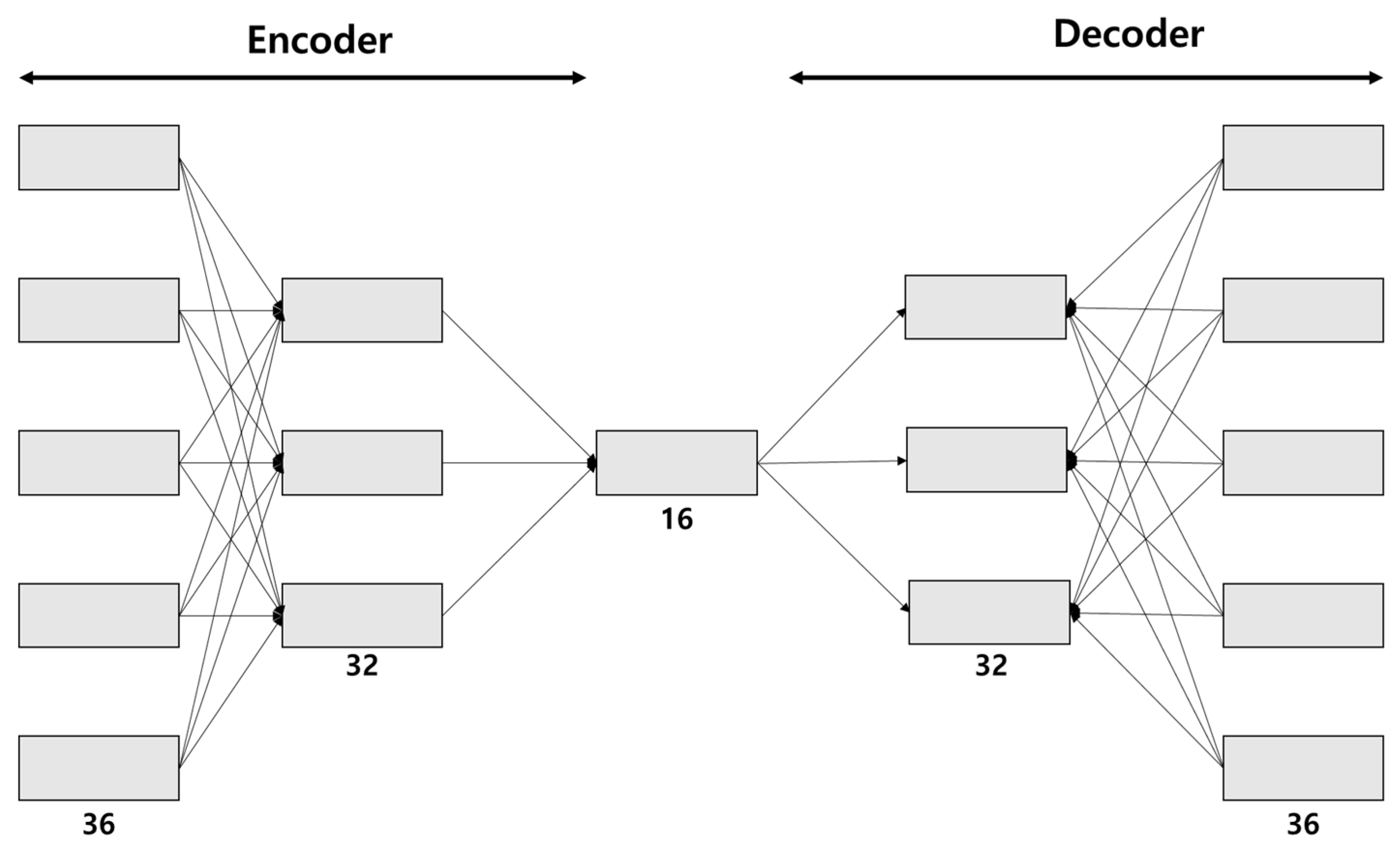
AE is a technique of unsupervised learning that learns patterns in data. An encoder takes in data and compresses them until they reach latent space while extracting key patterns in the data. The decoder has a learning method to reconstruct the low-dimensional compressed data by restoring them to their original dimensions. The key to distinguishing between anomalies in the AE algorithm is to restore the compressed data and compare them to the input data. Equation (2) means that the input dataset $x$ is compressed and mapped to the low-dimensional dataset $f\left(x\right)$.

$$z=f\left(x\right)$$

(8)

In the above formula, $z$ represents the value of the key pattern in the input dataset that is extracted during the compression process. $f\left(x\right)$ represents the function of the encoder, which compresses the dataset. $x$ is represented by the input data. Rectified Linear Unit (ReLU) is a non-linear function that enables neural networks to capture non-linear patterns in data, which is crucial for modeling complex relationships. Unlike activation functions like Sigmoid or Tanh, ReLU does not suffer from the vanishing gradient problem, especially for large input values. As a result, ReLU is commonly used as the activation function in neural networks. The formula for reconstructing the compressed data by restoring them is given by Equation (3).

$$x^{\prime }=g\left(z\right)$$

(9)

In Equation (3), $x^{\prime }$ represents the data that have been compressed and then restored by the decoder. $g\left(z\right)$ represents the decoder function responsible for reconstructing the compressed data. The reconstruction error is obtained through $x$ and $x^{\prime }$, which were obtained earlier, and AE learns to reduce the reconstruction error. The corresponding value is given by Equation (4).

$$Reconstruction Error={‖x-x^{\prime }‖}_2^2$$

(10)

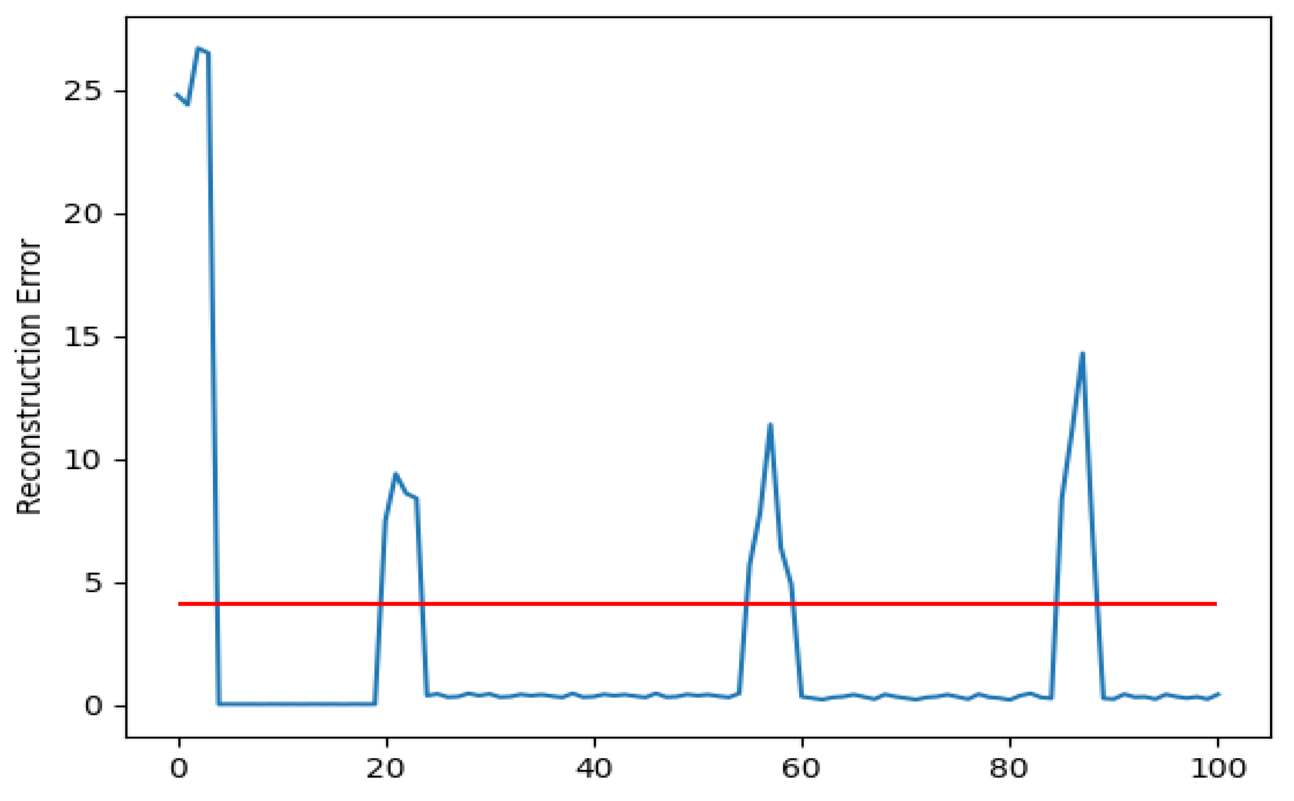
In the above formula, $‖·‖$ stands for $L_{2}norm$. The equation represents the reconstruction loss of an Autoencoder and is used for detecting anomalies. The reconstruction loss measures the distance between the original dataset $x$ and the reconstructed dataset $x^{\prime }$, and when the difference between them is significant, it is considered an anomaly. Therefore, if the reconstruction loss exceeds a certain threshold, the data are classified as an anomaly [34].

AE is a more powerful model for dimensionality reduction and feature extraction than other deep learning models. In anomaly detection, it is important to detect and extract specificity, and AE is very good at doing this. In addition, it has a relatively simple structure and can prevent overfitting and improve generalization performance, so in this study, AE was used to perform anomaly detection.

3. BGP Dataset Description and Anomaly Detection Environment

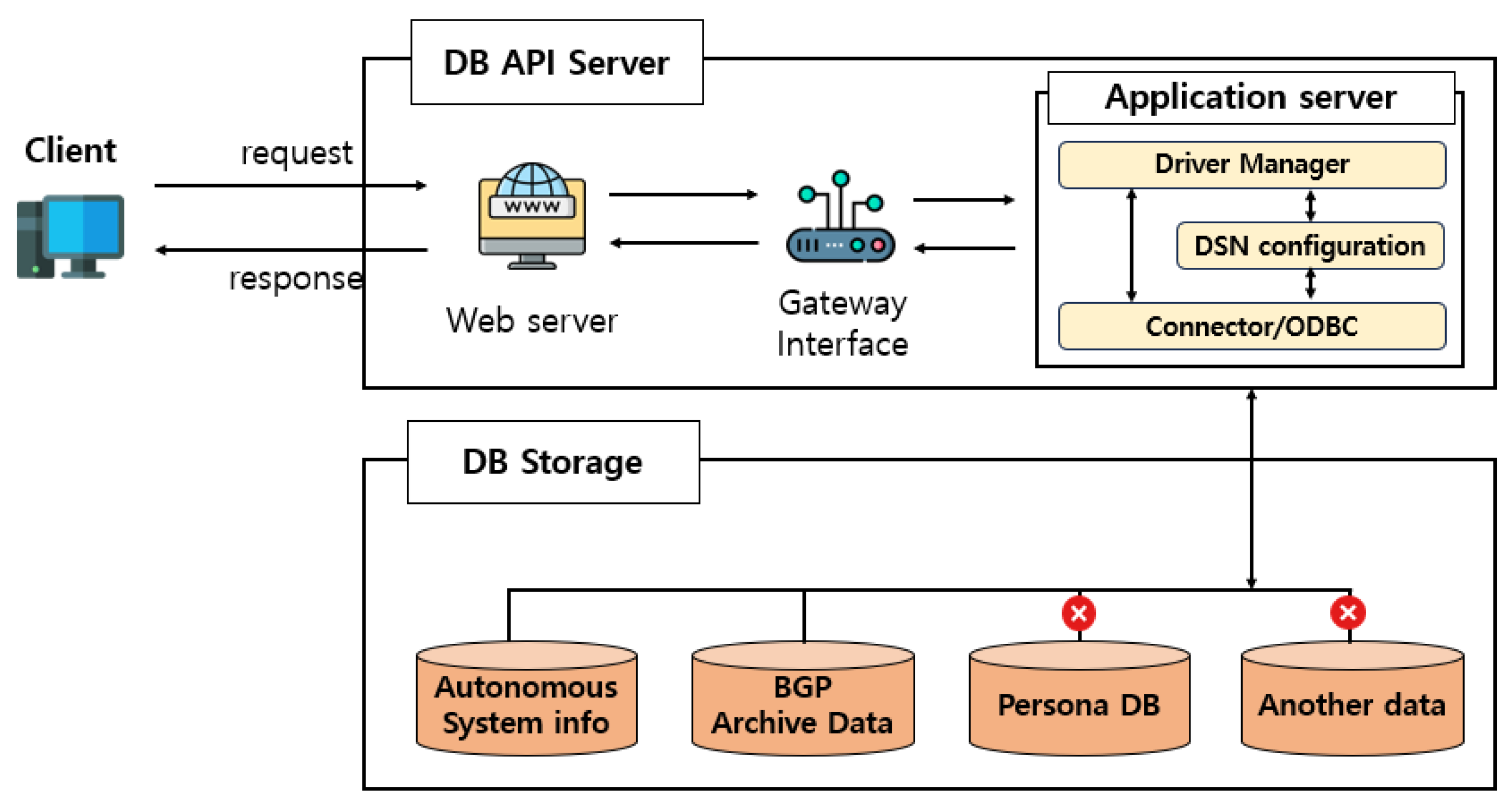
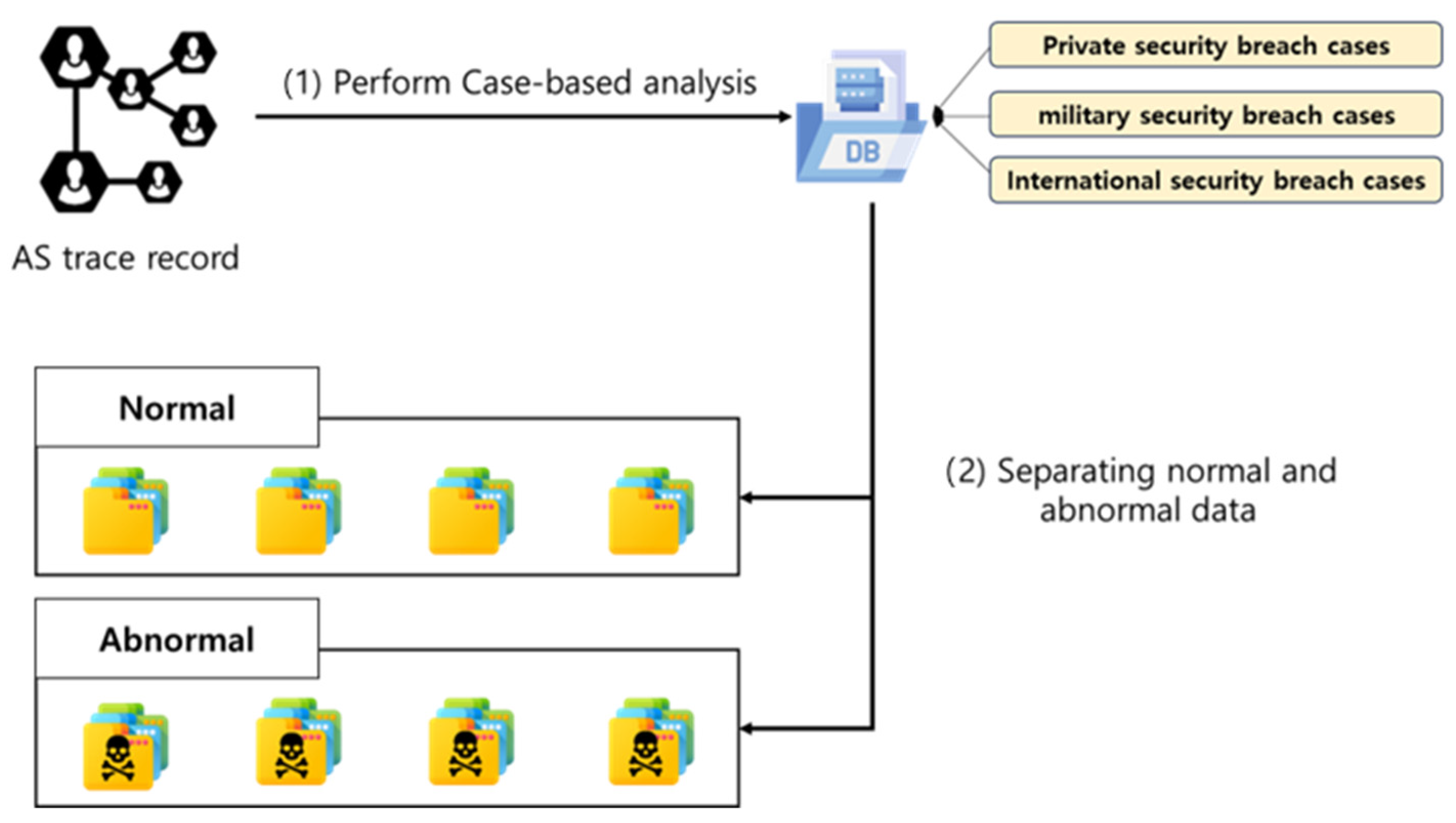
In this study, In this study, Figure 3 shows the structure of the AE used in this paper, showing that the dimensionality decreases in the encoder and increases in the decoder. Figure 4 and Figure 5 illustrate the process of collecting BGP data to detect anomalies in cyberspace. In Figure 4, the client requests data from the DB API Server, and the DB API Server collects data by sending BGP data containing AS information to the client. Figure 5 shows the AS trace records of the collected data compared to the security incident cases and separates them into normal and abnormal data. Normal data refer to AS that have no record of cyberattacks, while abnormal data refer to AS that have frequently attempted cyberattacks.

The data have been collected, labeled normal and abnormal, and are presented in

Table 2. Some of the normal and abnormal data in BGP data.

Timestamp	Peer IP	Peer AS	Path	Location	Label
16 September 2022	212.66.96.212	20,912	A -> C -> D	Italy	1
16 September 2022	12.0.1.63	7018	U -> F -> E	US	0
16 September 2022	37.139.139.17	57,866	H -> U -> A	Netherland	1
17 September 2022	194.153.0.2	5413	L -> C -> A	Australia	0
17 September 2022	198.129.33.85	293	U -> A -> D	US	0
…	…	…	…	…	…

. A detailed description of each attribute can be found in

Table 3. BGP dataset column definitions.

Column	Definition
Timestamp	Time information that indicates when routing data were sent or received. It is usually combined with date and time information to show the exact time an event occurred.
Peer Ip	An IP address between two devices or systems that communicate back and forth in a network environment. Each device has a unique IP address, which allows it to identify its owner.
Peer AS	When sending and receiving communications in a network environment, it refers to the number of the AS that sent the communication. Like IPs and carriage numbers, AS numbers have a unique identification number that identifies the owner.
Path	Information about which AS a dataset packet traversed to reach its destination.
Location	Information about the country of ownership of the peer AS.
Label	Distinguish between normal and abnormal data. 0: Normal data 1: abnormal data

. The criteria for selecting abnormal data were based on irregular changes in the path of a peer AS that frequently attempted attacks. For instance, abnormal data were classified when a suspected target, which typically follows the path sequence ‘A -> B -> C’, suddenly changed to ‘A -> D -> E -> F’.

The classification of normal and abnormal data is based on a threshold value exceeding a certain limit, as depicted in Figure 6. Abnormal data typically involve sudden AS path changes and the emergence of new path patterns, resulting in significantly elevated reconstruction values for the corresponding data points. The reconstruction error is determined using statistical properties such as the mean and standard deviation of the training data. It is decided by selecting a specific percentile or a multiple of the standard deviation as the threshold.

4. Experiments

In this section, experiments were conducted using the previously mentioned preprocessed data and machine learning algorithms, and the results are described.

4.1. BGP Dataset Preprocessing with Tokenizer

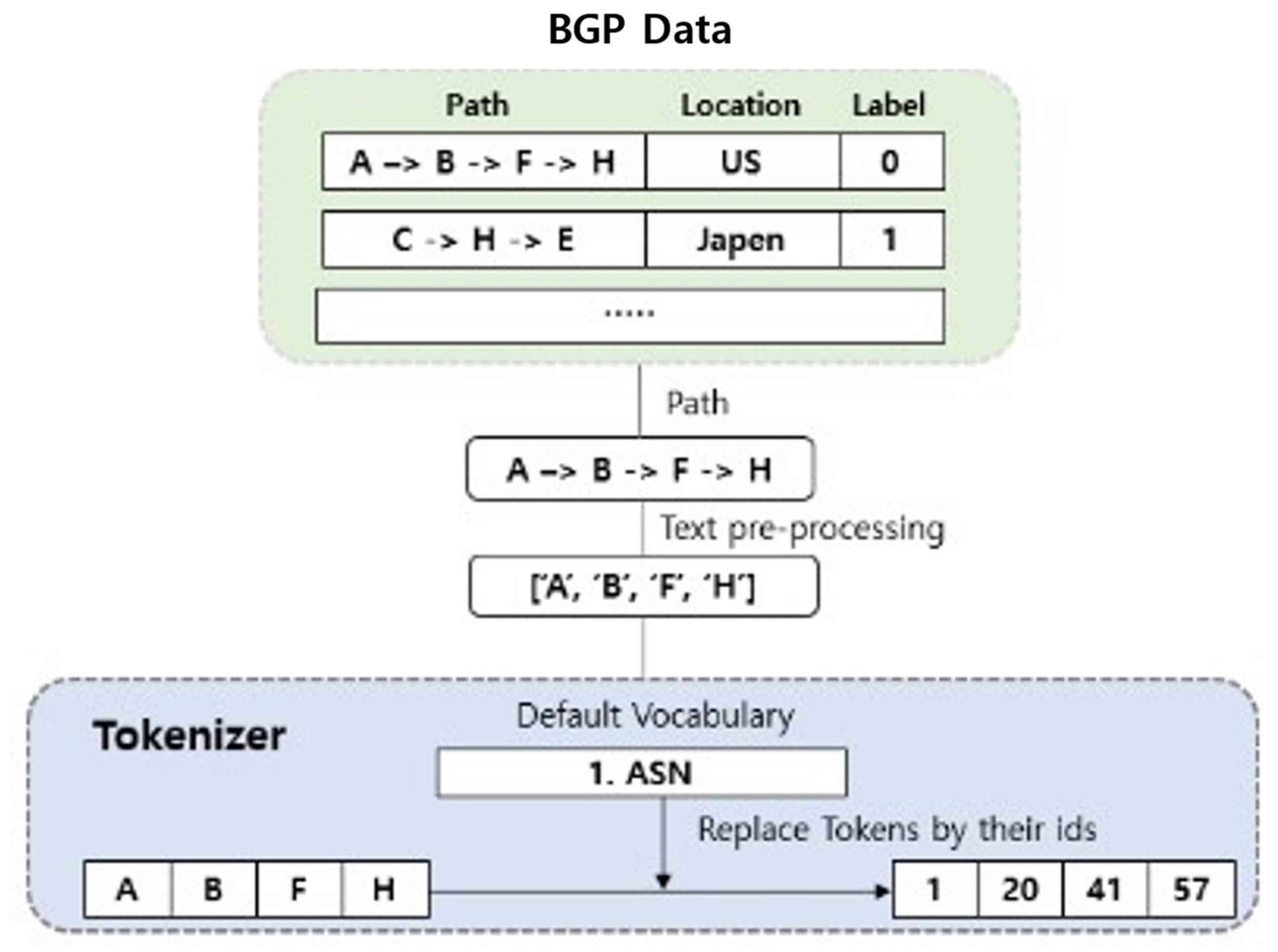
Machine learning algorithms can only learn from numeric data. However, as shown in Table 2, path and location are character data, so the models cannot learn them. To solve the above problem, preprocessing needs to be performed. Figure 7 illustrates the process of converting text data into numeric data through a tokenizer.

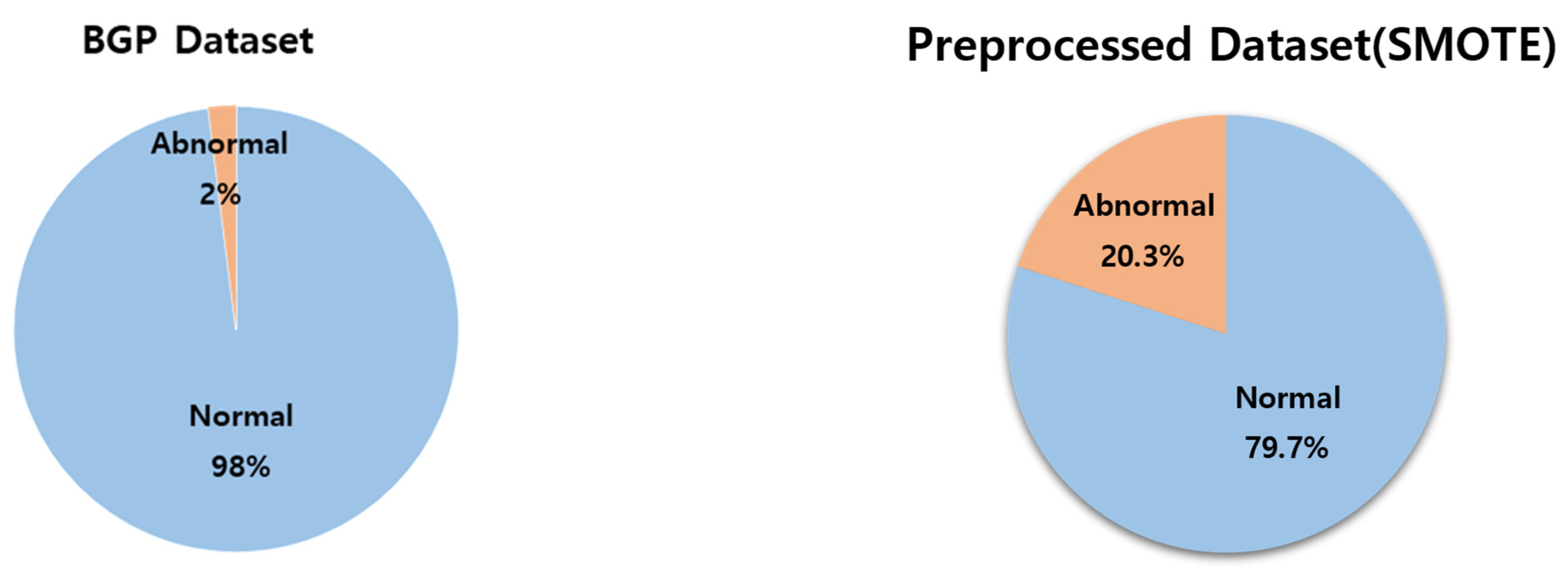
In this process, the sequence is split by dividing the string into smaller units. An example would be breaking down a path like ‘A -> B -> F -> H’ into individual components: [‘A’, ‘B’, ‘F’, ‘H’]. Finally, dataset preprocessing is completed by assigning unique integer numbers to the separated path characters. Figure 8 displays the dataset distribution of the preprocessed data in a pie chart. It can be observed that there has been a significant change in the ratio of normal to abnormal data. There are a variety of techniques to address dataset imbalances.

Generative Adversarial Networks (GANs) or Variational Autoencoders (VAEs) can be considered effective methods for dealing with imbalance issues, but their models focus on mimicking the distribution of the data. This means that they generate fewer abnormal data than normal data. Furthermore, these models are not suitable as anomaly detection models because their main purpose is to generate data according to their distribution, not to detect anomalies.

Undersampling is a technique where instances are randomly removed from many classes, which may result in the loss of potentially valuable information and patterns present in the majority of class data [35].

The resampling method increases the number of data in the minority category to make it equal to the number of data in the majority category, but it has the disadvantage of causing overfitting in the minority category [36].

Adaptive Synthetic Sampling (ADASYN) is a technique designed to overcome the limitations of SMOTE. It places its emphasis on generating synthetic samples based on the density distribution of minority-class instances. However, it demands additional resources and meticulous parameter tuning due to increased complexity, and it has the potential to introduce misinformation by oversampling mislabeled data points [37].

To solve this issue, the Synthetic Minority Oversampling Technique (SMOTE) is employed, which is one of the techniques used for balancing dataset imbalances. SMOTE works by identifying the nearest neighbors of the samples from the minority class and generating synthetic data points between these neighbors and the minority class sample [35,36]. The generated data are added to the original dataset, and anomaly detection is performed using the combined data, with the generated data labeled as anomalies. The process continues to repeat until the dataset’s needs are met. The result of applying SMOTE is shown on the right side of Figure 8. The rationale for maintaining an 8:2 ratio of normal to abnormal data is that elevating the number of abnormal dataset instances to attain a 5:5 ratio of normal to abnormal data can blur the boundaries between the normal and abnormal classes. Such blurring can lead to issues with the model misclassifying normal data as abnormal data. Additionally, an excessive application of SMOTE can lead the model to learn patterns from the generated data rather than capture patterns within the actual abnormal data, potentially undermining the model’s performance.

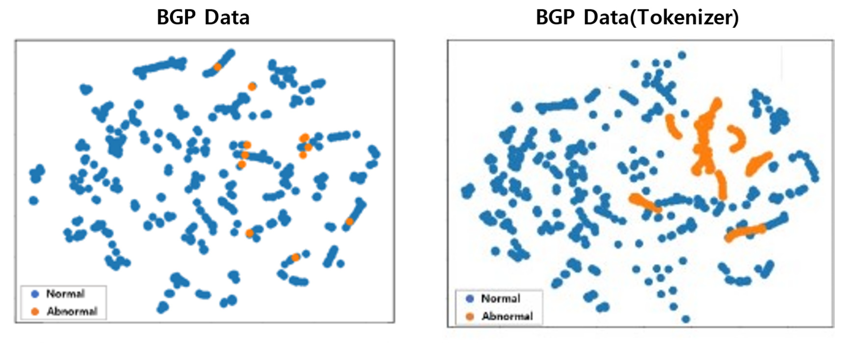
Understanding dataset distribution before model training is deemed crucial. PCA serves the purpose of visualizing data by reducing dimensionality. However, it encounters challenges when dealing with non-linear patterns and complex clusters. On the other hand, t-distributed Stochastic Neighbor Embedding (t-SNE) conquers these limitations by adeptly preserving intricate structures, making it highly effective for high-dimensional, non-linear data [38,39]. Figure 9 illustrates how BGP data and SMOTE are efficiently distributed using t-SNE, especially for anomalies, ultimately enhancing dataset analysis and visualization. Figure 9 displays the distribution of the BGP data and SMOTE after applying t-SNE. Upon examining the dataset distribution after preprocessing on the right, it can be observed that the anomalies are clustered to the right, with a few of them mixed in with the normal data. However, the original data exhibit almost no anomalies. With t-SNE, it can be observed that, during preprocessing, anomalies are adequately distributed from the original data, with few anomalies.

4.2. Parameters and Performance Evaluation of Models

The BGP dataset comprises a total of one million data points. To mitigate the vanishing gradient problem associated with an abundance of training and testing data, twenty thousand data points were allocated for training, and an additional 20,000 were set aside for testing, following preprocessing with SMOTE and tokenization. Throughout the training phase, the model acquired patterns and features from the regular data. Subsequently, in the experiments conducted using the test data, data points with high reconstruction error values that did not match the patterns and characteristics of normal data were classified as anomalies. The RF, One-SVM, CNN–LSTM, and AE algorithms were experimented with using both BGP datasets as training and test data. The parameters that make up the AE, RF, One-SVM, and CNN–LSTM algorithms are presented in

Table 4. AE parameters used in the experiment.

Parameters	AE Value
Epoch	100
Batch size	32
Activation Function	LeaklyReLu, Linear
Optimizer	Adam
Loss Function	MSE

,

Table 5. RF parameters used in the experiment.

Parameters	RF Value
N_estimaotors	100
Max_depth	None
Min_sample_split	3
Min_sample_leaf	2
Max_features	‘auto’
bootstrap	True

,

Table 6. One-SVM parameters used in the experiment.

Parameters	One-SVM Value
kernel	‘rbf’
nu	0.05
gamma	1.0
degree	4
Shrinking	True
Cache size	500
Random state	None

and

Table 7. CNN–LSTM parameters used in the experiment.

Parameters	One-SVM Value
Convolutional Filters	64
Convolutional Kernel	3 × 3
Convolutional Activation	ReLU
Max Pooling Size	2
LSTM Units	100
LSTM Activation	tanh
Dropout Rate	0.2
Dense Activation	ReLU
Output Activation	sigmoid
Loss Function	Binary Crossentropy
Optimizer	Adam

, and the experimental environment is shown in

Table 8. Anomaly detection experiment environment.

Equipment	Name
OS	Window 11 pro
CPU	Intel(R) Core 19-13900K
RAM	32 GB
GPU	NVIDIA GeForce RTX 4080 SUPER 16 GB
Language	Python 3. 6. 4
Libraries	TensorFlow, scikit-learn, Pandas

.

The purpose of this experiment is to learn the AS path patterns of abnormal and normal AS and detect abnormal behavior using BGP data. In anomaly detection problems, there can be an imbalance in the ratio of normal data to abnormal data. For instance, when outlier data occur exceptionally rarely, the model might tend to classify all data as normal. In such scenarios, relying solely on accuracy can lead to a high accuracy rate, but it may result in missing out on crucial abnormal data. To evaluate the performance of the models utilized in the experiments, various metrics were employed, each defined as follows:

• Precision: The percentage of data in the experiment that correctly identified the abnormal AS path as an abnormal AS path. This metric assesses the accuracy of the model’s classification of anomaly data.
• Recall: It, also known as “sensitivity” or “true positive rate”, represents how well the model correctly identifies true abnormal AS paths. For example, if the recall is 0.9, it means that the model misses 10% of the true abnormal AS paths.
• F1-Score: It is computed as the harmonic mean of precision and recall, providing a balanced measure in datasets with class imbalances where one class is dominant. This metric comprehensively assesses the model’s performance by considering false positives and false negatives. A high F1 score indicates a well-balanced trade-off between precision and recall, signifying the model’s ability to accurately classify both positive and negative samples.
• Receiver Operation Characteristic (ROC) Curve: One of the methods used to visualize the performance of binary classification models. This curve represents the relationship between the False Positive Rate (FPR) and True Positive Rate (TPR) as the threshold of the classification model is adjusted. The ROC curve plots the FPR on the x-axis and the TPR on the y-axis, showing the model’s performance at different thresholds. The TPR is equivalent to the recall and represents the proportion of true positive samples correctly classified as positive. On the other hand, the FPR represents the proportion of false–positive samples incorrectly classified as positive.

The above metrics are calculated based on the confusion matrix. It is shown in

Table 9. Confusion matrix.

		Actual Values
		Positive	Negative
Predicted Values	Positive	TP	FP
	Negative	FN	TN

and the metrics are calculated using Equations (11)–(15).

• True Positive (TP): A metric that represents the number of correctly classified positive samples in a binary classification model. These are the samples that the model correctly identified as positive when they were positive, meaning the model made accurate positive predictions. TP is a crucial indicator of the model’s performance, helping to assess its ability to correctly detect positive instances in the dataset.
• True Negative (TN): A metric used in binary classification to represent the number of correctly classified negative samples by the model. These are the samples that the model accurately identified as negative when they were indeed negative, indicating that the model made correct negative predictions. TN is an important measure of the model’s performance, assessing its ability to correctly identify and exclude negative instances in the dataset.
• False Positive (FP): Measures the frequency of the anomaly detection model incorrectly predicting normal data as anomalies, i.e., the model incorrectly categorizes normal instances as anomalies.
• False Negative (FN): Indicates the number of times the anomaly detection model incorrectly predicted abnormal data as normal.
• TPR: The percentage of abnormal data that the model correctly classified as anomalous out of the actual abnormal data.
• FPR: The percentage of normal data that the model misclassifies as abnormal data.

$$Precision=\frac{TP}{TP+FP}$$

(11)

$$Recall=\frac{TP}{TP+FN}$$

(12)

$$F1\text{-}Score=2· \frac{Precisiojn ·Recall}{Precision+Recall}$$

(13)

$$TPR=\frac{TP}{TP+FN}$$

(14)

$$FPR=\frac{FP}{FP+TN}$$

(15)

4.3. Experiments Results

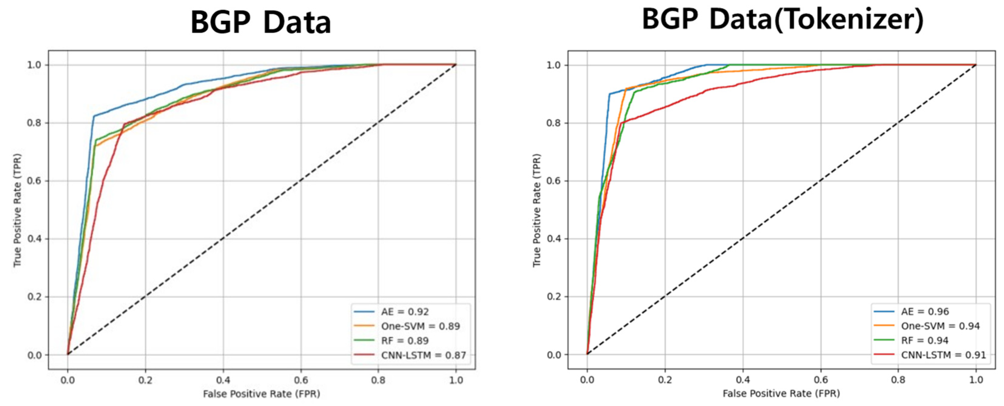
The experimental results were evaluated by measuring the AUROC to assess the accuracy of normal and abnormal dataset classifications. The AUROC value ranges from 0 to 1, with 0.5 indicating a random classifier and 1 indicating a perfect classifier. A higher AUROC value implies better classification performance, with values closer to 1 indicating a more accurate and reliable model for distinguishing between positive and negative classes. AUROC is particularly useful when dealing with imbalanced datasets or when the cost of false positives and false negatives differs significantly.

Table 10. AUROC Measurement Results.

Models	BGP Data	BGP Data (Tokenizer)
RF	0.893	0.944
One-SVM	0.892	0.946
CNN–LSTM	0.873	0.914
AE	0.927	0.961

presents a summary of the AUROC performance of the BGP data used in our experiments. The unprocessed data achieved performance ranging between 89% and 92%, while the preprocessed data with tokenizer achieved performance ranging between 91% and 96%, indicating a performance difference of approximately 3.7%.

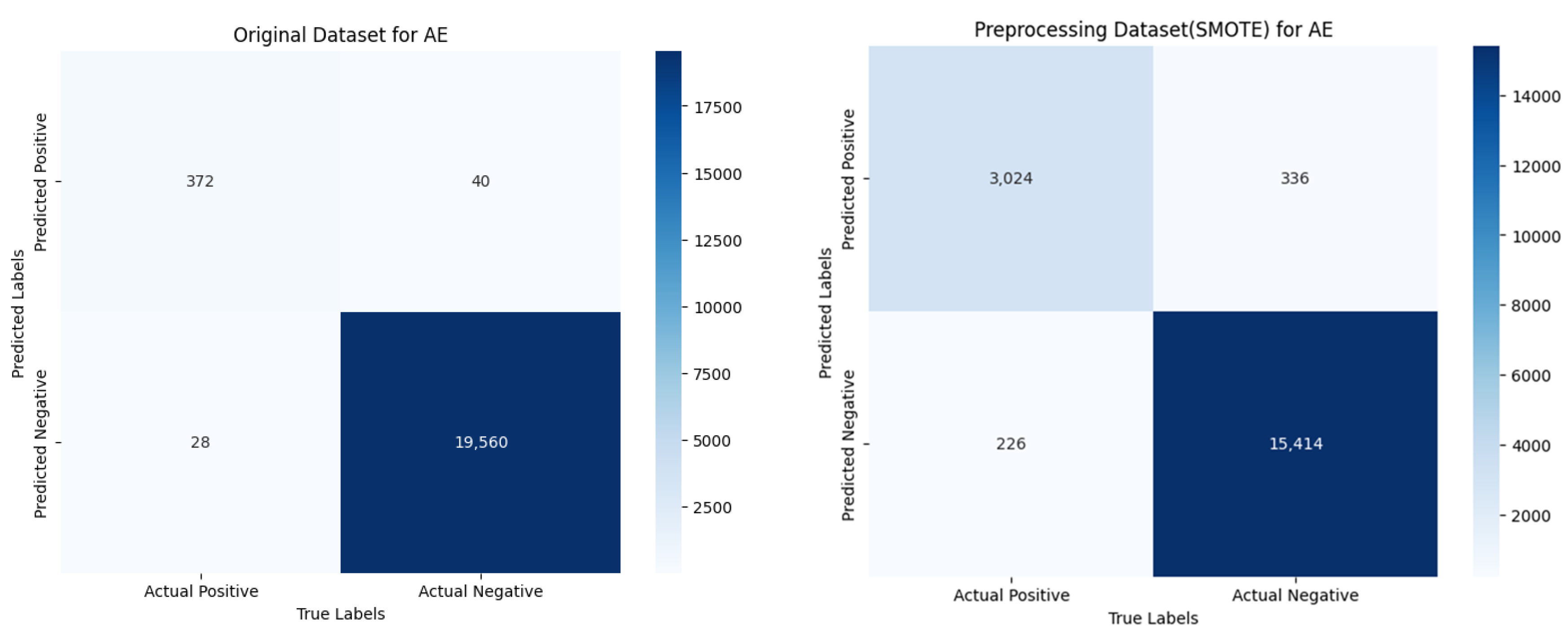
Figure 10 shows the AUROC values of the machine learning models, and the experimental results are shown in

Table 11. Abnormal dataset detection results from BGP data.

Models	Precision	Recall	F1-Score
CNN–LSTM	0.82	0.84	0.83
One-SVM	0.8	0.85	0.83
RF	0.86	0.89	0.87
AE	0.9	0.93	0.9

and

Table 12. Abnormal dataset detection results from BGP data using the tokenizer.

Models	Precision	Recall	F1-Score
CNN–LSTM	0.90	0.92	0.92
NB	0.93	0.94	0.93
RF	0.95	0.93	0.97
AE	0.98	0.99	0.99

. The results demonstrate that the BGP data with tokenizers significantly outperformed the original BGP data. Particularly in the case of AE, all indicators increased significantly from 0.89 to 0.97, and overall, all metrics improved. Figure 11 is an image representing the confusion matrix results after applying AE. In both scenarios, when calculating accuracy, it appears to be 0.99. However, the results obtained through auxiliary indicators indicate that overfitting occurred in the unprocessed BGP data.

5. Conclusions

In this study, an experiment was conducted to identify anomalies using machine learning and BGP data. Machine learning algorithms, including AE, One-SVM, RF, and CNN–LSTM, were employed to classify the data into normal or anomalous categories. To unify the form of the data, tokenizer preprocessing was used to convert character data into numerical data, and the SMOTE technique was applied to address the issue of dataset imbalance. To quantify the performance of the model, various secondary metrics, such as AUROC, were utilized to provide objective numbers. The results demonstrated that the BGP data preprocessed with the tokenizer outperformed the original BGP data in all cases. Among them, tokenizer-preprocessed BGP data performed the best, achieving an AUROC of 0.96 and an accuracy of 0.99 in anomaly detection through AE. This result shows the best results among experiments that use machine learning to detect abnormalities in BGP data and confirms that overfitting has been prevented.

By using the results, the potential for real-time cyber anomaly detection and identifying the rerouting of previously identified malicious users to enable ongoing monitoring is presented. Additionally, the preprocessing method used in this research is a very challenging study that applies NLP-based tokenizer techniques not used in existing BGP data. Furthermore, by employing the above techniques and utilizing SMOTE, this study demonstrated the enhanced capability of machine learning in detecting abnormal behaviors in cyberspace. Finally, to detect cyber anomalies, anomalies were detected using BGP data. The detection abilities of accuracy (0.99), precision, recall, f1-score, and AUROC curves were 0.98, 0.99, 0.99, and 0.96, respectively, showing that overfitting did not occur.

In future research, BGP data will be compared with other data to check for consistency. Then, data will be fused to utilize various attributes such as system logs, network traffic, and user behavior data instead of only AS routes. To overcome the limitations of AS path data and develop a more comprehensive detection model, attack types will also be added to the breach case information to create a model that can detect each attack type. Moreover, the model’s performance will be enhanced through the combination of deep learning algorithms and novel preprocessing techniques, resulting in improved detection capabilities.

References

1. Check Point: Third Quarter of 2022 Reveals Increase in Cyberattacks and Unexpected Developments in Global Trends. Available online: https://blog.checkpoint.com/2022/10/26/third-quarter-of-2022-reveals-increase-in-cyberattacks/ (accessed on 26 April 2023).
2. Scott, K.D. Joint Publication (JP) 3–12 Cyberspace Operation; The Joint Staff: Washington, DC, USA, 2018. [Google Scholar]
3. Ahn, G.; Kim, K.; Park, W.; Shin, D. Malicious file detection method using machine learning and interworking with MITRE ATT&CK framework. Appl. Sci. 2022, 21, 10761. [Google Scholar]
4. Rekhter, Y.; Li, T.; Hares, S. A Border Gateway Protocol 4 (BGP-4); No. rfc4271; Internet Engineering Task Force: Fremont, CA, USA, 2006. [Google Scholar]
5. Lad, M.; Massey, D.; Pei, D.; Wu, Y.; Zhang, B.; Zhang, L. PHAS: A Prefix Hijack Alert System. In Proceedings of the 15th USENIX Security Symposium, Vancouver, BC, Canada, 31 July–4 August 2006; p. 3. [Google Scholar]
6. Comarela, G.; Crovella, M. Identifying and analyzing high impact routing events with PathMiner. In Proceedings of the 2014 Conference on Internet Measurement Conference, Vancouver, BC, Canada, 5–7 November 2014; pp. 421–434. [Google Scholar]
7. McGlynn, K.; Acharya, H.B.; Kwon, M. Detecting BGP route anomalies with deep learning. In Proceedings of the IEEE INFOCOM 2019-IEEE Conference on Computer Communications Workshops (INFOCOM WKSHPS), Paris, France, 29 April–2 May 2019; pp. 1039–1040. [Google Scholar]
8. Chen, Z.; Yeo, C.K.; Lee, B.S.; Lau, C.T. Autoencoder-based network anomaly detection. In Proceedings of the 2018 Wireless Telecommunications Symposium (WTS), Phoenix, AZ, USA, 17–20 April 2018; IEEE: Piscataway, NJ, USA, 2018. [Google Scholar]
9. Copstein, R.; Zincir-Heywood, N. Temporal representations for detecting BGP blackjack attacks. In Proceedings of the 2020 16th International Conference on Network and Service Management (CNSM), Izmir, Turkey, 2–6 November 2020; IEEE: Piscataway, NJ, USA, 2020; pp. 1–7. [Google Scholar]
10. Choudhary, S.; Kesswani, N. Analysis of KDD-Cup’99, NSL-KDD and UNSW-NB15 datasets using deep learning in IoT. Procedia Comput. Sci. 2020, 167, 1561–1573. [Google Scholar] [CrossRef]
11. Zhang, J.; Zheng, Y.; Qi, D.; Li, R.; Yi, X. DNN-based prediction model for spatio-temporal data. In Proceedings of the ACM Sigspatial International Conference on Advances in Geographic Information Systems, San Francisco, CA, USA, 31 October–3 November 2016. [Google Scholar]
12. Moustafa, N.; Slay, J. UNSW-NB15: A comprehensive data set for network intrusion detection systems (UNSW-NB15 network data set). In Proceedings of the 2015 Military Communications and Information Systems Conference (MilCIS), Canberra, Australia, 10–12 November 2015; pp. 1–6. [Google Scholar]
13. Dhanabal, L.; Shantharajah, S. A study on NSL-KDD dataset for intrusion detection system based on classification algorithms. Int. J. Adv. Res. Comput. Commun. Eng. 2015, 4, 446–452. [Google Scholar]
14. Tavallaee, M.; Bagheri, E.; Lu, W.; Ghorbani, A.A. A detailed analysis of the KDD CUP 99 data set. In Proceedings of the IEEE Symposium on Computational Intelligence for Security and Defense Applications (CISDA), Ottawa, ON, Canada, 8–10 July 2009; pp. 1–6. [Google Scholar]
15. Ji, Y.; Lee, H. Event-Based Anomaly Detection Using a One-Class SVM for a Hybrid Electric Vehicle. IEEE Trans. Vehic. Technol. 2022, 71, 6032–6043. [Google Scholar] [CrossRef]
16. Sarah, M.E.; Rajasegarar, S.; Karunasekera, S.; Leckie, C. High-dimensional and large-scale anomaly detection using a linear one-class SVM with deep learning. Pattern Recognit. 2016, 58, 121–134. [Google Scholar]
17. Halbouni, A.; Gunawan, T.; Habaebi, M. CNN-LSTM: Hybrid Deep Neural Network for Network Intrusion Detection System. IEEE Access 2022, 10, 99837–99849. [Google Scholar] [CrossRef]
18. Yulianto, A.; Sukarno, P.; Suwastika, N.A. Improving Adaboost-Based Intrusion Detection System (IDS) Performance on CIC IDS 2017 Dataset. In Proceedings of the 2nd International Conference on Data and Information Science, Bandung, Indonesia, 15–16 November 2018; Volume 1192, p. 012018. [Google Scholar]
19. Almomani, I.; Al-Kasasbeh, B.; Al-Akhras, M. WSN-DS: A Dataset for Intrusion Detection Systems in Wireless Sensor Networks. J. Sens. 2016, 2016, 4731953. [Google Scholar] [CrossRef]
20. Kim, T.Y.; Cho, S.B. Web Traffic Anomaly Detection Using C-LSTM Neural Networks. Expert Syst. Appl. 2018, 106, 66–76. [Google Scholar] [CrossRef]
21. Wright, R.E. Logistic regression. In Reading and Understanding Multivariate Statistics; American Psychological Association: Washington, DC, USA, 1995. [Google Scholar]
22. Muniyandi, A.P.; Rajeswari, R.; Rajaram, R. Network anomaly detection by cascading k-Means clustering and C4. 5 decision tree algorithms. Procedia Eng. 2012, 30, 174–182. [Google Scholar] [CrossRef]
23. Anton, S.D.D.; Sinha, S.; Schotten, H.D. Anomaly-based intrusion detection in industrial data with SVM and random forests. In Proceedings of the 2019 International Conference on Software, Telecommunications and Computer Networks (SoftCOM), Split, Croatia, 19–21 September 2019; pp. 1–6. [Google Scholar]
24. Morris, T.H.; Thornton, Z.; Turnipseed, I. Industrial control system simulation and data logging for intrusion detection system research. In Proceedings of the 7th Annual Southeastern Cyber Security Summit, Huntsville, AL, USA, 3–4 June 2015; pp. 3–4. [Google Scholar]
25. Anton, S.D.; Gundall, M.; Fraunholz, D.; Schotten, H.D. Implementing scada scenarios and introducing attacks to obtain training data for intrusion detection methods. In Proceedings of the ICCWS 2019 14th International Conference on Cyber Warfare and Security: ICCWS 2019, Stellenbosch, South Africa, 28 February–1 March 2019; Academic Conferences and Publishing Limited: Berkshire, UK, 2019; p. 56. [Google Scholar]
26. Zhang, X.; Gu, C.; Lin, J. Support vector machines for anomaly detection. In Proceedings of the 2006 6th World Congress on Intelligent Control and Automation, Dalian, China, 21–23 June 2006. [Google Scholar]
27. Breiman, L. Random forests. Mach. Learn. 2001, 45, 5–32. [Google Scholar] [CrossRef]
28. Yassin, W.; Udzir, N.I.; Muda, Z.; Sulaiman, M.N. Anomaly-based intrusion detection through k-means clustering and naives Bayes classification. In Proceedings of the 4th International Conference on Computing and Informatics, ICOCI, Kuching, Malaysia, 28–30 August 2013; Volume 49, pp. 298–303. [Google Scholar]
29. Zhang, J.; Zulkernine, M.; Haque, A. Random-forests-based network intrusion detection systems. IEEE Trans. Syst. Man Cybern. 2008, 38, 649–659. [Google Scholar] [CrossRef]
30. Sun, H.; Chen, M.; Weng, J.; Liu, Z.; Geng, G. Anomaly Detection for In-Vehicle Network Using CNN-LSTM with Attention Mechanism. IEEE Trans. Veh. Technol. 2021, 70, 10880–10893. [Google Scholar] [CrossRef]
31. Liu, Y.; Kumar, N.; Xiong, Z.; Lim, W.Y.B.; Kang, J.; Niyato, D. Communication-Efficient Federated Learning for Anomaly Detection in Industrial Internet of Things. In Proceedings of the 2020 IEEE Global Communications Conference, Taipei City, Taiwan, 7–10 December 2020; Volume 2020, pp. 1–6. [Google Scholar]
32. Li, K.L.; Huang, H.K.; Tian, S.F.; Xu, W. Improving one-class SVM for anomaly detection. In Proceedings of the 2003 International Conference on Machine Learning and Cybernetics (IEEE Cat. No. 03EX693), Xi’an, China, 5 November 2003; Volume 5, pp. 3077–3081. [Google Scholar]
33. Perdisci, R.; Gu, G.; Lee, W. Using an Ensemble of One-Class SVM Classifiers to Harden Payload-based Anomaly Detection Systems. In Proceedings of the Sixth International Conference on Data Mining (ICDM’06), Hong Kong, China, 18–22 December 2006; pp. 488–498. [Google Scholar]
34. Tschannen, M.; Bachem, O.; Lucic, M. Recent advances in autoencoder-based representation learning. In Proceedings of the Third Workshop on Bayesian Deep Learning (NeurIPS 2018), Montréal, QC, Canada, 7 December 2018. [Google Scholar]
35. Liu, X.-Y.; Wu, J.; Zhou, Z.-H. Exploratory undersampling for class-imbalance learning. IEEE Trans. Syst. Man Cybern. 2009, 39, 539–550. [Google Scholar]
36. Good, P.I. Resampling Methods; Springer: Boston, MA, USA, 2006. [Google Scholar]
37. He, H.; Bai, Y.; Garcia, E.A.; Li, S. ADASYN: Adaptive synthetic sampling approach for imbalanced learning. In Proceedings of the 2008 IEEE International Joint Conference on Neural Networks (IEEE World Congress on Computational Intelligence), Hong Kong, China, 1–8 June 2008; pp. 1322–1328. [Google Scholar]
38. Fernández, A.; Garcia, S.; Herrera, F.; Chawla, N.V. SMOTE for learning from imbalanced data: Progress and challenges, marking the 15-year anniversary. J. Artif. Intell. Res. 2018, 61, 863–905. [Google Scholar] [CrossRef]
39. Chawla, N.V.; Bowyer, K.W.; Hall, L.O.; Kegelmeyer, W.P. SMOTE: Synthetic minority over-sampling technique. J. Artif. Intell. Res. 2002, 16, 321–357. [Google Scholar] [CrossRef]
Figure 1. Random Forest Model (green as normal data and red as abnormal data).
Information 14 00501 g001
Figure 2. CNN–LSTM structure.
Information 14 00501 g002
Figure 3. Autoencoder structure.
Information 14 00501 g003
Figure 4. Data collection process.
Information 14 00501 g004
Figure 5. The process of classifying normal and abnormal data based on case analysis.
Information 14 00501 g005
Figure 6. Reconstruction error value.
Information 14 00501 g006
Figure 7. Preprocessing of BGP data.
Information 14 00501 g007
Figure 8. Dataset ratio pie graphs.
Information 14 00501 g008
Figure 9. Visualize dataset distributions with t-SNE.
Information 14 00501 g009
Figure 10. AUROC curve results.
Information 14 00501 g010
Figure 11. Confusion matrix results using AE.
Information 14 00501 g011