Abstract
Benchmarking different optimization algorithms is tasky, particularly for network-based cellular communication systems. The design and management process of these systems involves many stochastic variables and complex design parameters that demand an unbiased estimation and analysis. Though several optimization algorithms exist for different parametric modeling and tuning, an in-depth evaluation of their functional performance has not been adequately addressed, especially for cellular communication systems. Firstly, in this paper, nine key numerical and global optimization algorithms, comprising Gauss–Newton (GN), gradient descent (GD), Genetic Algorithm (GA), Levenberg–Marguardt (LM), Quasi-Newton (QN), Trust-Region–Dog-Leg (TR), pattern search (PAS), Simulated Annealing (SA), and particle swam (PS), have been benchmarked against measured data. The experimental data were taken from different radio signal propagation terrains around four eNodeB cells. In order to assist the radio frequency (RF) engineer in selecting the most suitable optimization method for the parametric model tuning, three-fold benchmarking criteria comprising the Accuracy Profile Benchmark (APB), Function Evaluation Benchmark (FEB), and Execution Speed Benchmark (ESB) were employed. The APB and FEB were quantitatively compared against the measured data for fair benchmarking. By leveraging the APB performance criteria, the QN achieved the best results with the preferred values of 98.34, 97.31, 97.44, and 96.65% in locations 1–4. The GD attained the worst performance with the lowest APE values of 98.25, 95.45, 96.10, and 95.70 in the tested locations. In terms of objective function values and their evaluation count, the QN algorithm shows the fewest function counts of 44, 44, 56, and 44, and the lowest objective values of 80.85, 37.77, 54.69, and 41.24, thus attaining the best optimization algorithm results across the study locations. The worst performance was attained by the GD with objective values of 86.45, 39.58, 76.66, and 54.27, respectively. Though the objective values achieved with global optimization methods, PAS, GA, PS, and SA, are relatively small compared to the QN, their function evaluation counts are high. The PAS, GA, PS, and SA recorded 1367, 2550, 3450, and 2818 function evaluation counts, which are relatively high. Overall, the QN algorithm achieves the best optimization, and it can serve as a reference for RF engineers in selecting suitable optimization methods for propagation modeling and parametric tuning.
1. Introduction
In recent years, the system design, deployment, and management of wireless radio frequency (RF) networks have become more tasking and complicated [1,2,3]. The intricacies and complications may be attributed to many dynamic factors. The advancement and constant evolution of different cellular network technologies, accompanied by different deployment procedures and management costs, can be a prominent factor [4,5,6]. In addition, frequent changes in localized environmental features such as houses, buildings, and trees, plus the varying weather condition around these networks, can be another significant factor [7,8,9].
Constant increasing traffic of mobile subscribers in the networks with different multimedia service quality demands could also be a key factor [10,11,12]. Remarkably, cell site acquisition is becoming more problematic due to the limited availability of suitable sites in a built-up area and neighboring residents that generally work against such site installations, probably because of frequently rumored electromagnetic radiations that emanate from them [13].
In order to cope with or overcome the aforementioned key challenges, the RF engineers must also be ready to explore techniques and efforts at the network design/deployment phase or optimization/management phase when in operation [14,15,16]. The propagation loss model is a key tool that the RF employs to estimate the cell radius and signal attenuation losses during and after cellular system network design/deployment [17]. These signal propagation models usually contain some unknown parameters that must be accurately determined in correspondence with experimental data from the terrain of interest. Inaccuracies in RF propagation modeling and their parameter estimation can compromise effective network planning, management, optimization, and operational activities [18,19,20]. The impact can be enormous regarding poor service quality, resource input wastage, and time costs. This key problem is often called the propagation model parameters identification problem in the telecommunication network engineering domain.
The field of predictive analytics has revolutionized decision-making processes across various industries by providing valuable insights and forecasts based on historical data. It involves the application of statistical models, machine learning algorithms, and optimization techniques to extract patterns and trends from data, enabling organizations to make informed decisions and predictions. Optimization algorithms play a crucial role in enhancing the accuracy and efficiency of predictive analytics by finding the optimal values of model parameters. Accurate modeling and estimating parametric values for cellular network-based propagation models is a dynamic optimization problem due to the different nonlinearities involved [21,22,23]. The interaction of the transmitted waves with different propagation mediums and terrain features around the receiver causes its strength to attenuate and degrade, thus resulting in what is known as signal propagation loss. During the cellular radio frequency (RF) network design or optimization phase of an existing one, the RF engineer uses signal propagation models to estimate the characteristics of signal attenuation losses that occur between the transmitting stations and the receiver stations [24,25,26]. These signal propagation models usually contain some unknown parameters that must be accurately determined in correspondence with experimental data from the terrain of interest.
Inaccuracies in RF propagation modeling and their parameter estimation can compromise effective network planning, management, optimization, and operational activities [27,28]. The impact can be enormous regarding poor service quality, resource input wastage, and time costs [29,30]. In the telecommunication network engineering domain, this key problem is often called the propagation model parameters identification problem [31,32].
Several numerical and global optimization methods exist in the literature [33,34,35,36], explored and published by different authors or researchers to tackle the intricate propagation model parameter identification problem. While various optimization algorithms in the literature attempt to tackle this key issue, selecting the preeminent one during application in solving a specific problem a priori is often difficult. Particularly, a methodical-based approach to benchmark the performance of diverse optimization algorithms to tackle the intricate radio propagation modeling and parametric tuning problems is currently missing, and the few studies available in the literature provided conflicting findings.
This paper identifies and provides an overview of the common existing numerical and global optimization methods. In order to assist a practicing scientist or an RF engineer in selecting the most suitable optimization algorithm for solving the parametric model tuning problem, the second focus is to introduce three-fold benchmarking criteria. The third focus is to explore benchmark criteria for the precision performance of the identified numerical and global optimization methods with practical case studies from different radio signal propagation terrains. Thus, the core contributions of this paper are as follows:
- We provide a clear-cut identification and detailed overview of the common existing numerical and global optimization algorithms.
- Introduction of three-fold benchmarking criteria, namely the Accuracy Profile Benchmark (APB), Function Evaluation Benchmark (FEB), and Execution Speed Benchmark (ES)
- Using the two-fold set of benchmarking criteria, we benchmarked the precision performance of the identified numerical and global optimization algorithms with practical case studies from different radio signal propagation terrains.
The remaining part of this paper is described as follows. Section 2 covers the related work. Section 3 describes the materials and methods, focusing on the identified optimization algorithms and their experimentation. Section 3 also presents the developed three-fold set of benchmarking criteria, while Section 4 provides the results and valuable discussions. Finally, the conclusion is given in Section 5.
2. Related Works
Different benchmarking and comparative works exist on numerical and global optimization performance impacts for real-time applications but not within the domain of intricate RF propagation modeling and parameter tuning problems. In [37], deterministic local and stochastic global optimization methods were investigated and compared to identify and estimate unknown kinetic model parameters systematically.
This paper identifies and provides an overview of the common existing numerical and global optimization methods. The second focus is to benchmark the precision performance of the identified numerical and global optimization methods with practical case studies from different radio signal propagation terrains. In [34], both stochastic and deterministic global optimization algorithms were studied for nonlinear biological modeling and parameter estimation. The stochastic methods provided lower processing time from their results but with poor convergence to a global minimum under a limited iteration number. On the contrary, the deterministic methods yielded preferred solutions regarding convergence quality but huge computational weights.
Several global optimization algorithms are benchmarked with standard functions for practical applications, presented in [33]. The authors discovered that the Hybrid Differential Evolution and Adaptation Evolution Strategy Algorithm was better for complex objective functions than the Hook–Jeeves and particle swam optimization, which attained better global minimum convergence for less complex objective functions.
In [38], five different global optimization algorithms were investigated for benchmarking to reconstruct and optimize nano-optical shape parameters. From the investigation, the Bayesian optimization method was reported to outperform other algorithms, such as differential evolution and particle swam, in terms of run times. A similar approach involving different optimizers is presented in [39] for the panel data model. It found that the computational success rate of the optimizers varies proportionally with the nature of the problem being handled by them. In [36], the cumulative density function is explored as an indicator to benchmark the performance of stochastic global optimization algorithms on test data sets’ analysis. The result reveals that the algorithms with the pure random search performed preferably better.
In [40], numerical-based optimization techniques focusing on Levenberg–Marguardt (LM) and Gauss–Newton (GN) algorithms were investigated to compare their performance on the propagation model parameter optimization and prediction analysis. With the application focus on loss data taken from built-up areas, the results showed that the LM outperformed the GN in terms of precision accuracies. In [41], Particle Swarm Optimization (PSO) and random forest (RF) were applied comparatively to tune and identify the parameters of the signals’ attenuation models. The authors found that the PS method attained the most preferred precision performance by 22–25% across the study locations, using maximum absolute error as the indicator.
In [42], neural networks, support vector machine, and random forest were benchmarked with traditional path loss models like the COST 231-Walfisch Ikegami model and COST 231-Hata model. The authors disclosed that random forest yielded the best precision performance in path loss prediction.
Through the propagation modelling and benchmarking process, it was found in [43] that the proposed LightGBM model, which is a machine learning-based developed modelling algorithm, outperforms the empirical models by 65% in terms of prediction accuracy and decreased by 13 x in prediction time when matched with ray-tracing. The notable performance was achieved even with thin training data sets. Also, via detailed benchmarking processes in [41,44], the authors developed hybrid particle swarm–random forest and vector statistics–neural network models for propagation loss modeling and observed that their proposed models attained preferred prediction accuracies compared to traditional approaches.
In [45], the predictive modelling performance of four popular machine learning methods consisting of support vector regression, neural networks, gradient tree boosting, and random forest was compared with empirical path loss models after incorporating crossed walls’ number into them. From among the four learning-based methods engaged, the gradient tree boosting displayed the best generalization and prediction capacities.
3. Methods
This work adopts a four-phased methodology, as shown in Figure 1. The first phase highlights how the field test measurement campaign was conducted to acquire the relevant signal data used for the propagation loss model tuning and parameter identification. It also reveals the considered generic propagation model and its variables. This is followed by defining the genetic propagation model and its specific modeling variables. Phase three reveals the nine adopted optimization methods. Phase four provides the developed two-fold set of benchmarking criteria and the benchmarking results. The streamlined stepwise algorithm adopted to actualize the main goal of the paper is as follows:

Figure 1.
The adopted four-phased workflow.
- Identify the generic propagation model to be tuned and specify its key parameters, vector h, of the model to be tuned (optimized), and the iteration number, z.
- Define the initial guess parameters, n = (0,0 0), and set nfeval = 0.
- Define the complete objective function connecting the optimization parameters.
- Optionally, select the optimization solver and carefully stipulate the required options.
- Appraise the defined objective function E(h) and the possible constraints g(h) ≤ (n); nfeval = nfeval + 1.
- Introduce fair benchmarking criteria.
- Assess the convergence and precision performance of each method base in step (vi).
- If conditions are met, then stop; otherwise,
- Apply the search further directional of each optimization method for the parameter update.
- Assess the convergence and precision optimization of each method, else return to step 1.
3.1. Field Measurements
The signal path loss data sets were obtained using professional TEMS investigation test tools. The TEMS tools, containing the Map info, scanner, TEMS software, compass, TEMs pocket phones, an inverter, and a GPS, were all connected and driven inside a salon car to perform the signal loss data collection. With the configured and connected tools that can automatically access, verify, optimize, troubleshoot, and benchmark operational mobile cellular networks, we drove around four different eNodeB transmitters within the designated study locations in Port Harcourt City, Nigeria. The height of the eNodeB transmitters ranged between 26 and 34 m above sea level. The four transmitters belong to a commercial Long Term Evolution network service provider, and each operates at a 2600 MHz transmission frequency in the 20 MHz bandwidth.
We employed a continuous measurement procedure with the active handover, enabling us to acquire the signal loss data around every measurement location [46]. This process first accesses the eNodeB transmitter and carries out the physical measurements via automated call initiations and establishments. The acquired signal data were also programmed to be saved automatically in logfile format during the field test. After the test, the data sets were extracted for further processing using MAP info, an Excel spreadsheet, and MATLAB software. Data pre-preparation is a critical step toward attaining effective model tuning and optimization; in this paper, the wavelet preprocessing tool in the MATLAB computational environment was utilized to detect and cater to missing data and the measured channel signal noisy components.
3.2. The Generic Propagation Loss Model
The generic propagation model, also popularly termed the log-distance or free-space model, is designed for a free-space environment assuming no signal propagation impediment between the transmitting and receiving antenna [47,48]. It is mathematically described as
where , and designate the log-distance model, signal propagation distance, and signal propagation frequency, respectively.
Therefore, to cater to other environments, such as urban, sub-urban, and rural, there is a need for parametric model tuning. In order to accomplish this, Equation (1) can be re-written in the form of (2):
Here, it should be noted that Equation (2) is only modeled in the form of Equation (1). The two equations are not necessarily the same. Specifically, Equation (1) assumes an ideal scenario where there is no obstacle in the line of sight. In Equation (2), the picture of the actual environment is depicted where path loss is expected due to the dynamic characteristics of the environment investigated. In practice, the values of , , and , in Equation (2), are not known until they are observed via theoretical simulation or experimentation. Depending on the environment and other dynamic environmental or man-made conditions, the values , , and , in Equation (2), will differ. This work is focused on obtaining these values for the scenarios considered as shown in the results section. In the ideal scenario, following Equation (1), these values are , , and = 20, and these cannot be used as a benchmark for the expected values in Equation (2). However, in Equation (2), the values of , , and would show very sharp or significant variations compared to the values in Equation (1). The values obtained for Equation (2) depict the real conditions of the environment examined, whereas those obtained for Equation (1) represent the ideal case, which is not possible in practice.
In this paper, Equation (2) is thus termed as a generic propagation model where , and define parameters to be tuned for a given environment. Lastly, it should be noted that any of the parameters, , and , may be negative depending on the scenario as observed in the results of the current study.
3.3. The Objective Function
Generally, optimization algorithms can be defined as mathematical procedures that search for the optimal solution of a given problem based on certain criteria or objective function. In propagation model tuning, the goal is to identify and determine the parameters , and in correspondence with the measured signal propagation loss. This can be attained in the least square sense, resulting in the main optimization problem. The literature has several numerical or global algorithms or methods of solving parametric optimization problems. The focus of this paper is to identify and provide an overview of the common existing numerical and global optimization ones with the sole aim of examining their propagation model parameters, identification, and tuning capabilities. The second focus is to benchmark the precision performance of the identified numerical and global optimization methods with practical case studies from different radio signal propagation terrains.
Objective functions play a fundamental role in parametric optimization and predictive modeling, providing a quantitative measure of the performance or quality of a solution. They are essential in predictive modeling as they drive the process of model optimization. They also serve as the guiding principle for optimization algorithms, helping to identify the optimal solution that satisfies specific constraints and maximizes desired objectives. In general, the choice of objective function depends on the problem at hand. In this paper, the parametric minimization objective function [44,46] is engaged. The objective function defines and houses the nonlinear path loss model we seek to minimize by means of numerical and global optimization algorithms. In general, our goal is driven by solving the vital parametric propagation modelling problem using the parametric optimization-based objective function [44,46], as shown in Figure 2, and it can be articulated mathematically as
where , represents the parameters of the targeted generic propagation model, .
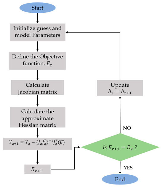
Figure 2.
Workflow for the numerical approach.
In Equation (3), ,, and n express the measured propagation loss variables, the target responses, generic propagation model, and measurement data points. The objective function in (3) is also engaged to harmonize the different components of the optimization problem, helping us to achieve the optimal outcome. By evaluating the objective function, we can compare candidate solutions and determine which ones are better or worse.
3.4. Numerical Method
Numerical optimization algorithms are like a diverse group of superheroes, each with their own superpowers to conquer specific problems. There is the trusty gradient descent, who relentlessly searches for the steepest downhill path. The numerical method applied is briefed in this section. First, the gradient descent is considered, and the direct search is described.
3.4.1. Gradient Descent (GD)
The gradient (g), Hessian (H), and Jacobian (J) of the optimization function in Equation (1) can be described using
By means of and H, the respective Gauss–Newton (GN), gradient descent (GD), Levenberg–Marquardt (LM), and Trust-Region–Dog-Leg (TR) solution to the optimization problem can be expressed as
where and denote the LM damping factor and identity matrix. The trial step, , defines the TR radius, with expressing the Dog Leg path that connects to the Cauchy point.
Instead of the Hessian matrix in Equation (4), the Quasi-Newton (QN) method uses an approximate Hessian and it is given with
The propagation model parameters are determined from each of the methods and their iterative updates as follows:
where z indicates the iteration number, and the QN approximate Hessian, , is given with
All of the parametric update is iteratively realized by employing the various algorithms in correspondence with the objective function, which houses the generic propagation model and the measured propagation loss values sequentially until a convergence termination is reached.
3.4.2. Direct Search
Here, the pattern search is considered. Pattern search (PAS) is the direct search algorithm for solving optimization problems. Unlike the numerical optimization algorithms that use higher derivatives or gradient information to search for the desired optimal point, the PAS does not require such information to drive the objective function. Rather, the PAS engages a set of point or rational basis vectors to probe or search the desired direction in the corresponding target objective function with the current mesh size. To implement the PAS algorithm in MATLAB, we use the solver caller technique, which is given with (22).
where objFun designates the objective function in Equation (1), Nvars indicate the model parameter number, and lob and upb define the lower and upper bound implementation constraints. The options constitute mesh size, accelerator, tolerance, and search method. The mesh tolerance controls the mesh size. For example, the solver stops if the mesh size exceeds the tolerance level.
SolPAS = pattersearch(objFun,nvars,lob,upb,[],options)
Set the mesh tolerance to 1 × 10⁻⁷, 10 times smaller than the default value. This setting can increase the number of function evaluations and iterations and lead to a more accurate solution.
3.5. Global Optimization Methods
Generally, global optimization methods play a crucial role in predictive analytics by enabling the discovery of optimal models, parameters, or configurations. They help in maximizing the accuracy of predictive models, minimizing error rates, and optimizing performance metrics. By efficiently exploring the entire solution space, these algorithms ensure that the best possible solution is achieved, leading to more accurate predictions and better decision making. While the numerical-based algorithms are driven by derivative or differential gradient and Hessian functions, the global optimization method depends on population sets [49,50]. Also, unlike local optimization algorithms that rely on starting from an initial solution and making incremental improvements, global optimization algorithms explore multiple solutions simultaneously to find the best outcome. Particularly, the global algorithms come in where exact numerical algorithms fail. The following global optimization methods consisting of Genetic Algorithm (GA), particle swam (PS), and Simulated Annealing (SA) are also considered in this paper. The Genetic Algorithms mimic the process of natural selection to find the fittest solution. These algorithms, along with others like Simulated Annealing and Particle Swarm Optimization, bring a touch of magic to the world of optimization.
3.5.1. Genetic Algorithms (GAs)
The GA is a classic global-search and evolutionary computation-based algorithm developed by Holland [51,52,53] to solve optimization problems regarding objective function maximization or minimization using the concept of natural selection in genetics. Particularly, in GA, a population or pool of possible candidate solutions made to undergo selection, recombination, and mutation are engaged to produce new ones [19,54]. In this process, each candidate solution (or individual) is allocated a fitness value in correspondence with the given objective function value, and the process is repeated over a generation of individuals until a global optimum solution is attained or a stopping convergence criterion is reached.
Unlike the numerical techniques, the GA does not use any derivative information to solve real-world optimization problems. However, one key problem with GA is that it might not converge to the desired or near-usable optimum solution if the implementation process is not done properly. To implement the GA algorithm in MATLAB, we use the solver caller technique, which is given with (23).
where objFun designates the objective function, Nvars indicate the model parameter number, and lob and upb define the lower and upper bound implementation constraints. The options constitute the population size, generation number, crossover value, Elite count, and selection function.
solGA = ga(objFun,nvars,lob,upb,[],options)
3.5.2. Particle Swarm (PS)
The PS is a bio-inspired computational algorithm proposed by the authors of [52,55] to provide distinctive solutions to optimization problems through iterative search space. It was specifically developed to mimic a flock of birds or a school of fish that moves together in a group while flying or swimming randomly to receive the best hunt as they search for food. To implement the PS algorithm in MATLAB, we use the solver caller technique, which is given with (24).
where objFun designates the objective function in Equation (24), Nvars indicate the model parameter number, and lob and upb define the lower and upper bound implementation constraints. The options constitute the swarm size, the iteration number, the Inertial range, the Social Adjustment Weight, and the maximum iteration number.
Solps = particleswarm(objFun,Nvars,lob,upb,options)
3.5.3. Simulated Annealing
The SA is another global search-based optimization algorithm that uses how metals cool and anneal in metallurgy to solve diverse optimization problems. SA can be applied iteratively to resolve hard, unconstrained, or constrained computational optimization problems, particularly when exact numerical algorithms fail. At each iteration process, the SA algorithm generates a new random. Then, a distance of the trial point is selected from the present or earlier point using a probability distribution whose scale is dependent upon temperature in connection with the objective function, and by accepting the new points, the algorithm circumvents and skirts being stuck in local minima. As the temperature is lowered, the SA algorithm reduces the range and copes with its global search space to converge and attain a global minimum. To implement the SA algorithm in MATLAB, we use the solver caller technique, which is given with
where objFun designates the objective function in Equation (25), Po indicates the initial guess parameters, and lob and upb define the lower and upper bound implementation constraints. The options constitute the temperature information, simulannealbnd, the iteration number, and the plotting function. Table 1 gives the numerical/global model parameter optimization algorithms.
solSA = simulannealbnd(objFun, po,lob,upb, options)

Table 1.
Numerical/Global Model Parameter Optimization Algorithms.
3.6. Accuracy Profile Benchmark
It is crucial to establish an Accuracy Profile Benchmark (APB) to examine the objective tuning space optimality and accuracy of the respective optimization parametric tuning method. The APB can help profile the accuracy attained with each optimization method in reaching the desired performance while minimizing every relative error. Additionally, APB is needed to provide or reflect the performance index attained in evaluating the objective function toward reaching the parametric model tuning goal.
Here, the APB can be computed via
where MAPE defines the mean percentage error (or relative error) to be minimized during the parametric model tuning process. , k, and express the actual and the predicted values of ith quantity, with k being the quantity number in the parametric tuning model.
APB = 100 − MAPE
3.7. Function Evaluation Benchmark
Besides engaging the APB to profile the accuracy attained, each tuning method is involved in reaching the desired global or local solution. Thus, the total function evaluations achieved, which can help reveal the total search trials or mock-ups performed until the optimization tuning process is completed, are also crucial to be looked into. In order to benchmark using this technique, the total function evaluation number targeted is kept in the respective optimization method during the parametric tuning process. Informatively, we defined the Function Evaluation Benchmark (FEB) as
where k reveals the quantity number in the parametric model being tuned with the respective optimization method.
3.8. Execution Speed Benchmark
The speed with which each optimizer takes to achieve a reasonably swift converging solution with minimal error is tagged as the execution speed (ES). The ES, which can also be termed convergence speed, is related to the number of evaluations (NumEval) using
where CPU time defines the time used to run each optimizer code.
4. Results and Discussion
Objective functions are the driving force behind predictive modeling. They define what we are trying to predict and how we measure the accuracy of our predictions. By optimizing the objective function, we can fine-tune our models to improve their predictive power. Whether it is minimizing mean squared error or maximizing area under the curve, the objective function guides us toward building better models. The optimization algorithms drive the predictive mathematical procedures that search for the optimal solution of a given problem based on certain criteria or objectives. These algorithms help us find the best possible solutions in a vast search space. However, the strength of the respective optimization algorithms lies in their specific ability to save time, resources, and effort by finding the most efficient solutions. Whether it is maximizing profits, minimizing costs, or achieving optimal performance, these algorithms are like superheroes that can transform messy problems into elegant solutions. Therefore, benchmarking these algorithms arises when there is a clear need to compare the performance of algorithms fairly against certain standards during or after being applied to solve specific optimization problems or a particular set of problems. Thus, benchmarking is carried out here to appraise the respective nine algorithms’ capacity to solve the parametric propagation loss modeling and tuning problem in correspondence with the practical loss data from different terrains. To actualize this specific task, we explore the three-fold benchmarking criteria that can help reveal prediction accuracy and the objective function value described in Section 3.6 and Section 3.7. A smaller precision error and objective function value are preferred for a more precise solution.
4.1. Accuracy Profile Benchmark Analysis Using MAPE and APB
First is each optimization, and precision accuracy with the Mean Absolute Percentage Error (MAPE). In connection with the APB, as in Equations (27) and (28), the MAPE quantifies how close the attained prediction model values are to the observed or measured values. Accordingly, a smaller MAPE value indicates that the predicted values are very close to the measured field values. Similarly, a higher MAPE value indicates the predicted values are far apart from the measured field values. Accordingly, based on the benchmarking expressions in Equations (26) and (27), a smaller MAPE value or higher APB would indicate the most preferred optimization method concerning prediction parametric tuning.
The importance of optimization algorithms lies in their ability to save time, resources, and effort by finding the most efficient solutions toward achieving optimal accuracy. Whether it is maximizing profits, minimizing costs, or achieving optimal performance, these algorithms are like superheroes that can transform messy problems into elegant solutions. Figure 3, Figure 4, Figure 5 and Figure 6 show the prediction tuning accuracy with computed MAPE performance values attained with the GD, LM, GN, QN, TR, PAS, GA, PS, and SA when applied for the prediction modeling and parametric tuning of the generic propagation model. The results show the QN achieved the best results over other algorithms with the lowest MAPE values of 1.6319, 2.6909, 2.5676, and 2.6560 in locations 1–4. This was followed by the PS method with 1.6319, 2.7615, 2.5775, and 3.6558 in locations 1–4. The SA and PAS methods attained MAPE values 1.6321, 2.7731, 2.5793, 3.6590, 1.6336, 2.9592, and 2.5843 at the same locations, 1–4. The GD attained the worst performance with the highest MAPE values of 1.7482, 4.5987, 3.8946, and 4.2051 in the same four locations.
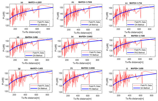
Figure 3.
Benchmarked optimization error analysis with MAPE in location 1.
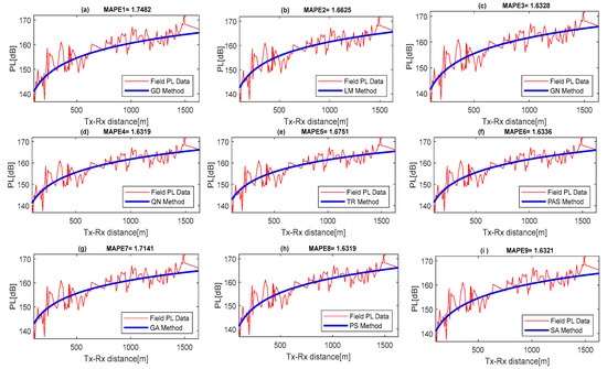
Figure 4.
Benchmarked optimization error analysis with MAPE in location 2.
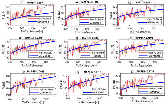
Figure 5.
Benchmarked optimization error analysis with MAPE in location 3.
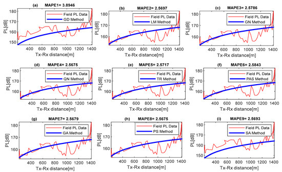
Figure 6.
Benchmarked optimization error analysis with MAPE in location 4.
Similarly, the QN method also accomplishes the preferred APB values of 98.34, 97.31, 97.44, and 96.64% at the same locations. The best parametric precision tuning results recorded with the proposed QN optimization method may imply that it can iteratively adjust the standard propagation loss values against the measured data more accurately than others. It may also clearly point out that the QN method owns better global convergent capacity during the parametric tuning process in correspondence with MAPE minimization, irrespective of the initial choices when starting to guess parameters. As mentioned earlier, the QN algorithm works by approximating the Hessian matrix, which represents the second-order derivatives of the objective function. It uses an iterative process to update the solution and converge toward the optimal values. The algorithm calculates gradients, adjusts the step sizes, and updates the solution based on the calculated increments. This iterative process continues until the algorithm reaches the convergence criteria or a maximum number of iterations. This efficiency allows analysts to quickly train and update predictive models, saving valuable time and resources.
4.2. Benchmarking with Objective Function Value Analysis
This subsection provides the objective function value analysis of the resultant solution attained when determining the propagation loss model parameters with the respective optimization method. A smaller objective function value is the most preferred solution and optimization algorithm. Figure 7, Figure 8, Figure 9 and Figure 10 and Table 2, Table 3, Table 4 and Table 5 display the objective function value results achieved with each optimization method versus the function evaluation count.
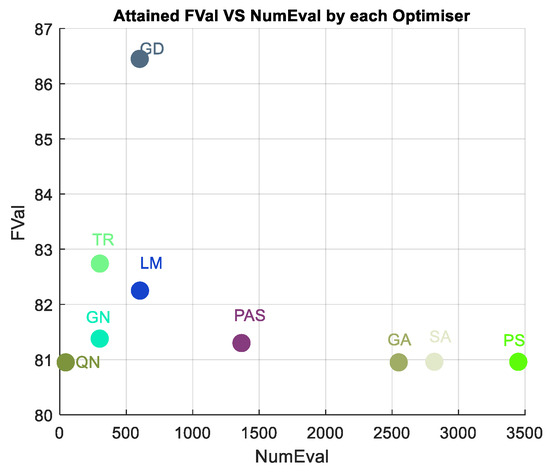
Figure 7.
Benchmarked algorithms with FVal analysis in location 1.
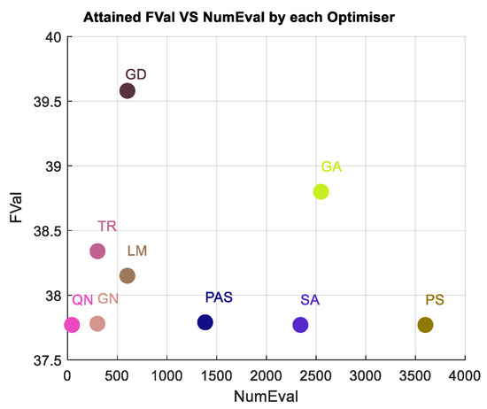
Figure 8.
Benchmarked algorithms with FVal analysis in location 2.
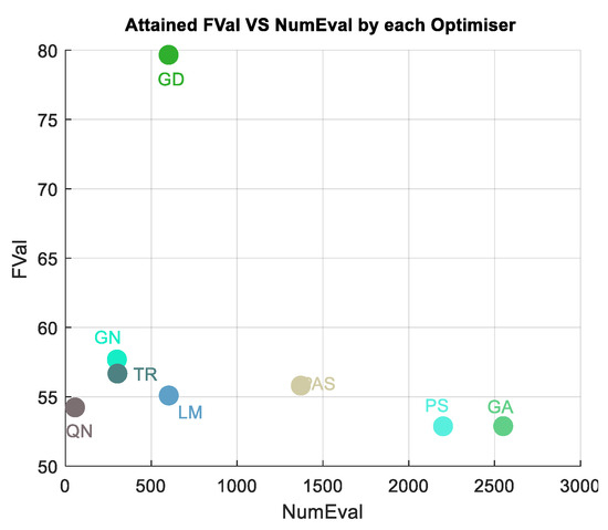
Figure 9.
Benchmarked algorithms with FVal analysis in location 3.
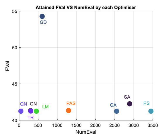
Figure 10.
Benchmarked algorithms with FVal analysis in location 4.

Table 2.
Estimated Parameters and the Attained FVal in Location 1.

Table 3.
Estimated Parameters and the Attained FVal in Location 2.

Table 4.
Estimated Parameters and the Attained FVal in Location 3.

Table 5.
Estimated Parameters and the Attained FVal in Location 4.
A key challenge in numerical and global optimization is the issue of convergence and local optima. Convergence refers to the point at which an algorithm stops searching and determines that it has found the best solution possible. However, algorithms can converge to local optima, which are good solutions within a limited region of the search space. Here, the function evaluation is engaged to count and reveals the number of evaluations (NumEval) that each optimization method iteratively underwent to reach their respective local or global solution after initiation. We can infer from the tables and the figures that the QN method owns the fewest function evaluation counts of 44, 44, 56, and 44, and the lowest objective value of 80.85, 37.77, 54.69, and 41.24, thus attaining the best optimization method across the study locations. This also implies the QN finds the best solutions by attaining the lowest objective function values across the study locations after iteratively tuning propagation loss model loss parameters. GA takes many more function evaluations than pattern searches. By chance, it arrives at a better solution.
Again, the worst performance is attained with GD with objective values 86.45, 39.58, 76.66, and 54.27, respectively, in the four study locations. Though the objective values achieved with global optimization algorithms such as PAS, GA, PS, and SA are relatively small, like the QN, their function evaluation counts are quite high. For example, in Table 1, the PAS, GA, PS, and SA recorded 1367, 2550, 3450, and 2818 function evaluation counts, which are quite high. Remarkably, the PS and GA took a higher order of magnitude in function evaluations to find the global optimum and arrived at good solutions of 80.96 objective values each, the same as the one attained with the QN method. Most global optimization algorithms are stochastic, population-based controlled ones, and their results change frequently or intermittently with every run. So, it takes those extra steps and time to run to completion, thus leading to higher objective function evaluation values. Compared to the gradient descent, the QN algorithm achieved a faster convergence rate, making it more suitable for large-scale data sets and time-sensitive tasks, and ideal for scenarios where time is a critical factor. This efficiency allows analysts to quickly train and update predictive models, saving valuable time and resources.
In general, each optimization method iterates to find an optimum. Each algorithm kick-starts with the initial value , then performs some relevant intermediary computations that ultimately lead to the new tuned point . The iterative tuning process continues repeatedly until the remaining parametric estimates and are determined after some z iteration number. The values of the parametric estimates attained with the studied nine optimization methods are shown in Table 2, Table 3, Table 4 and Table 5.
4.3. Benchmarking with Execution Speed
While the convergence speed quantifies how quickly the algorithm reaches an optimal solution, the executing speed (ES) expresses the rate taken for an optimizer to achieve a reasonably swift converging solution with minimal error and is used to evaluate the convergence speed attained with the benchmarking optimization methods. ES also helps reveal the rapt required to run the iterations and computational complexity in engaging during the parametric modeling and prediction algorithms in connection with the function evaluation number and the CPU time defined in Equation (29). Here, the reached execution speed (ES) engaged in assessing the convergence solution pace attained with each optimization algorithm is presented. The attained ES values displayed in Figure 11 reveal that the numerical-based optimization tuning methods achieved the fasted convergence over the global method, but again clearly showing that the QN method provides the best performance. While the GD, LM, TR, and GA maintained a constant level, GN, QN, PAS, PS, and SA algorithms displayed varied speeds across the study locations during optimization. The optimal performance of the QN may be ascribed to its ability to handle large-scale data sets, converge quickly, and adapt to noisy data, making it a suitable choice for many predictive analytics tasks. Therefore, compared to other optimization techniques, the Quasi-Newton algorithm offers a balance between efficiency and accuracy.
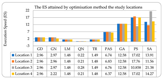
Figure 11.
Benchmarked algorithms with FVal analysis in locations 1–4.
While the numerical optimization focuses on finding the optimal solution to achieve minimal estimation error for a given problem within a defined range or domain, the global optimization algorithms explore the entire solution space to identify the optimal solution, taking into account potential multiple local optima that may exist to achieve the desired estimation error. Figure 12 reveals the channel-estimation error (averaged over the three h-parameters) versus data points for all estimation methods. In terms of maximum residual estimation error, the QN, GD, LM, TR, GA, GN, QN, PAS, PS, and SA algorithms attained 7.94, 7.92, 7.97, 7.90, 7.99, 7.95, 7.96, 7.91, and 7.92, respectively. These estimated error values also indicate the QN method narrowly outperforming others, particularly the PS, LM, and SA methods.
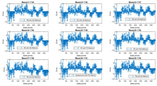
Figure 12.
Channel-estimation error (averaged over the three h-parameters) versus data points for all estimation methods.
5. Conclusions
This paper benchmarked nine numerical- and global-based optimization algorithms by comparing their precision performance on an intricate, multidimensional objective function involving the generic propagation model parameters and measured data. The optimization error (precision error) and the objective function value were critically assessed for fair performance benchmarking. A smaller optimization error and objective function value are most preferred for an optimal solution. Thus, in terms of precision error and the objective function value, the results show that the QN method achieved the least optimization error with MAPE values of 3.6319 in location 1, 2.6909 in location 2, 2.676 in location 3, and 3.6560 in location 4, providing the best prediction accuracies over other algorithms. But in terms of objective function values and their evaluation count, the QN algorithm attained the best values of 44, 44, 56, and 44, and the lowest objective value of 80.85, 37.77, 54.69, and 41.24, thus showing it as the best optimization algorithm for optimal propagation modeling and parametric tuning across the investigated locations. The robust performance of the QN can be traced to its capability to converge with few iterations and still easily find globally optimal solutions. The global optimization method keenly displays similar precision performance but at the cost of higher iteration update steps or counts. The gradient descent method displays the worst precision performance due to its poor scaled direction. Also, the gradient descent method is very sensitive to initial quest parameter choice. If the iteration step is large, it usually converges prematurely, thus leading to a suboptimal set of parameter identification, as seen in all results.
From our key findings, the worst performance is attained with the GD with objective values of 86.45, 39.58, 76.66, and 54.27, respectively. Though the objective values achieved with global optimization methods, PAS, GA, PS, and SA, are relatively small compared to the QN, their function evaluation counts are high. The PAS, GA, PS, and SA recorded 1367, 2550, 3450, and 2818 function evaluation counts, which are relatively high. Overall, the QN algorithm achieves the best optimization, and it can serve as a reference for RF engineers in selecting suitable optimization methods for propagation modeling and parametric tuning. Future work could focus on enhancing the signal predictability features of the presented models for optimal performance. Particularly, emerging technologies like 5G, Internet of Things (IoT), and massive Multiple Input Multiple Output (mMIMO) systems pose new challenges and opportunities for radio propagation modeling. These technologies require more accurate and efficient modeling techniques to handle the increased complexity of wireless networks and their interactions with various environments. The integration of machine learning and artificial intelligence techniques in radio propagation modeling can revolutionize the field. In addition, future work could engage the power of neural networks, deep learning, and reinforcement learning, as means to develop more sophisticated models that can adapt and learn from data, leading to more highly accurate and efficient predictions. Future work could also include the integration meta heuristic algorithms to tackle complex problems, and the development of adaptive and self-learning objective functions. Finally, embracing these future trends and directions would pave the way for enhanced wireless communication systems and a connected future.
Author Contributions
The manuscript was written through the contributions of all authors. J.I. was responsible for the conceptualization of the topic; article gathering and sorting were carried out by J.I., A.L.I., O.A.A., O.R.O. and E.O.; manuscript writing and original drafting and formal analysis were carried out by J.I., A.L.I., O.A.A., C.-C.L. and C.-T.L.; writing of reviews and editing were carried out by J.I., A.L.I., O.A.A., O.R.O., E.O., C.-C.L. and C.-T.L.; and J.I. led the overall research activity. All authors have read and agreed to the published version of the manuscript.
Funding
The work of Agbotiname Lucky Imoize is supported by the Nigerian Petroleum Technology Development Fund (PTDF) and the German Academic Exchange Service (DAAD) through the Nigerian-German Postgraduate Program under grant 57473408.
Institutional Review Board Statement
Not applicable.
Informed Consent Statement
Not applicable.
Data Availability Statement
The data that support the findings of this paper are available from the corresponding author upon reasonable request.
Acknowledgments
The authors thank the anonymous reviewers for the useful comments, which helped to improve the quality of the manuscript.
Conflicts of Interest
The authors declare no conflict of interest related to this work.
References
- Brenner, M.A. Radio Frequency Interference Monitor. U.S. Patent 7555262B2, 30 June 2009. [Google Scholar]
- Oh, H.S.; Jeong, D.G.; Jeon, W.S. Energy-efficient relay deployment in cellular systems using fractional frequency reuse and transmit antenna selection techniques. Int. J. Commun. Syst. 2019, 32, e3889. [Google Scholar] [CrossRef]
- Tataria, H.; Haneda, K.; Molisch, A.F.; Shafi, M.; Tufvesson, F. Standardization of Propagation Models: 800 MHz to 100 GHz—A Historical Perspective. 2020. Available online: http://arxiv.org/abs/2006.08491 (accessed on 15 October 2023).
- Bangerter, B.; Talwar, S.; Arefi, R.; Stewart, K. Networks and devices for the 5G era. IEEE Commun. Mag. 2014, 52, 90–96. [Google Scholar] [CrossRef]
- Viswanathan, H.; Mogensen, P.E. Communications in the 6G Era. IEEE Access 2020, 8, 57063–57074. [Google Scholar] [CrossRef]
- Mahmoodi, T.; Seetharaman, S. Traffic jam: Handling the increasing volume of mobile data traffic. IEEE Veh. Technol. Mag. 2014, 9, 56–62. [Google Scholar] [CrossRef]
- Yang, L.; Shami, A. On hyperparameter optimization of machine learning algorithms: Theory and practice. Neurocomputing 2020, 415, 295–316. [Google Scholar] [CrossRef]
- Shen, S.; Zhang, W.; Zhang, H.; Ren, Q.; Zhang, X.; Li, Y. An Accurate Maritime Radio Propagation Loss Prediction Approach Employing Neural Networks. Remote Sens. 2022, 14, 4753. [Google Scholar] [CrossRef]
- Nguyen, M.T.; Kwon, S.; Kim, H. Mobility robustness optimization for handover failure reduction in LTE small-cell networks. IEEE Trans. Veh. Technol. 2017, 67, 4672–4676. [Google Scholar] [CrossRef]
- Oueis, J.; Strinati, E.C. Uplink traffic in future mobile networks: Pulling the alarm. In Cognitive Radio Oriented Wireless Networks, Proceedings of the 11th International Conference, CROWNCOM 2016, Grenoble, France, 30 May–1 June, 2016; Springer: Berlin/Heidelberg, Germany, 2016; pp. 583–593. [Google Scholar]
- Caceres, N.; Wideberg, J.P.; Benitez, F.G. Review of traffic data estimations extracted from cellular networks. IET Intell. Transp. Syst. 2008, 2, 179–192. [Google Scholar] [CrossRef]
- Hwang, I.; Song, B.; Soliman, S.S. A holistic view on hyper-dense heterogeneous and small cell networks. IEEE Commun. Mag. 2013, 51, 20–27. [Google Scholar] [CrossRef]
- Fehske, A.; Fettweis, G.; Malmodin, J.; Biczok, G. The global footprint of mobile communications: The ecological and economic perspective. IEEE Commun. Mag. 2011, 49, 55–62. [Google Scholar] [CrossRef]
- Simon, G.; Volgyesi, P.; Maróti, M.; Ledeczi, A. Simulation-based optimization of communication protocols for large-scale wireless sensor networks. IEEE Aerosp. Conf. 2003, 3, 31339–31346. [Google Scholar]
- Alam, M.M.; Hamida, E.B. Strategies for optimal mac parameters tuning in ieee 802.15. 6 wearable wireless sensor networks. J. Med. Syst. 2015, 39, 106. [Google Scholar] [CrossRef] [PubMed]
- Imoize, A.L.; Udeji, F.; Isabona, J.; Lee, C.-C. Optimizing the Quality of Service of Mobile Broadband Networks for a Dense Urban Environment. Future Internet 2023, 15, 181. [Google Scholar] [CrossRef]
- Mohammadjafari, S.; Roginsky, S.; Kavurmacioglu, E.; Cevik, M.; Ethier, J.; Bener, A.B. Machine learning-based radio coverage prediction in urban environments. IEEE Trans. Netw. Serv. Manag. 2020, 17, 2117–2130. [Google Scholar] [CrossRef]
- Surajudeen-Bakinde, N.T.; Faruk, N.; Popoola, S.I.; Salman, M.A.; Oloyede, A.A.; Olawoyin, L.A.; Calafate, C.T. Path loss predictions for multi-transmitter radio propagation in VHF bands using Adaptive Neuro-Fuzzy Inference System. Eng. Sci. Technol. Int. J. 2018, 21, 679–691. [Google Scholar] [CrossRef]
- Valavanis, I.K.; Athanasiadou, G.E.; Zarbouti, D.; Tsoulos, G.V. Base-station location optimization for LTE systems with genetic algorithms. In Proceedings of the 20th European Wireless Conference, EW 2014, Barcelona, Spain, 14–16 May 2014; pp. 473–478. [Google Scholar]
- Lim, S.Y.; Yun, Z.; Iskander, M.F. Propagation measurement and modeling for indoor stairwells at 2.4 and 5.8 GHz. IEEE Trans. Antennas Propag. 2014, 62, 4754–4761. [Google Scholar] [CrossRef]
- Morita, Y.; Rezaeiravesh, S.; Tabatabaei, N.; Vinuesa, R.; Fukagata, K.; Schlatter, P. Applying Bayesian optimization with Gaussian process regression to computational fluid dynamics problems. J. Comput. Phys. 2022, 449, 110788. [Google Scholar] [CrossRef]
- Wilson, A.G.; Knowles, D.A.; Ghahramani, Z. Gaussian process regression networks. arXiv 2011, arXiv:1110.4411. [Google Scholar]
- Alali, Y.; Harrou, F.; Sun, Y. Optimized Gaussian Process Regression by Bayesian Optimization to Forecast COVID-19 Spread in India and Brazil: A Comparative Study. In Proceedings of the 2021 International Conference on ICT for Smart Society (ICISS), Bandung, Indonesia, 2–4 August 2021; pp. 1–6. [Google Scholar]
- Zakaria, Y.A.; Hamad, E.K.I.; Elhamid, A.S.A.; El-Khatib, K.M. Developed channel propagation models and path loss measurements for wireless communication systems using regression analysis techniques. Bull. Natl. Res. Cent. 2021, 45, 54. [Google Scholar] [CrossRef]
- Zeleny, J.; Perez-Fontan, F.; Pechac, P. Generalized propagation channel model for 2 GHz low elevation links using a ray-tracing method. Radioengineering 2015, 24, 1044–1049. [Google Scholar] [CrossRef]
- Aldhaibani, A.O.; Rahman, T.A.; Alwarafy, A. Radio-propagation measurements and modeling in indoor stairwells at millimeter-wave bands. Phys. Commun. 2020, 38, 100955. [Google Scholar] [CrossRef]
- Chan, C.C.; Kurnia, F.G.; Al-Hournani, A.; Gomez, K.M.; Kandeepan, S.; Rowe, W. Open-Source and Low-Cost Test Bed for Automated 5G Channel Measurement in mmWave Band. J. Infrared Millim. Terahertz Waves 2019, 40, 535–556. [Google Scholar] [CrossRef]
- Uwaechia, A.N.; Mahyuddin, N.M. A comprehensive survey on millimeter wave communications for fifth-generation wireless networks: Feasibility and challenges. IEEE Access 2020, 8, 62367–62414. [Google Scholar] [CrossRef]
- Liu, D.C.; Nocedal, J. On the limited memory BFGS method for large scale optimization. Math. Program. 1989, 45, 503–528. [Google Scholar] [CrossRef]
- Isabona, J. Joint Statistical and Machine Learning Approach for Practical Data-Driven Assessment of User Throughput Quality in Microcellular Radio Networks. Wirel. Pers. Commun. 2021, 119, 1661–1680. [Google Scholar]
- Popoola, S.I.; Atayero, A.A.; Faruk, N. Received signal strength and local terrain profile data for radio network planning and optimization at GSM frequency bands. Data Brief 2018, 16, 972–981. [Google Scholar] [CrossRef]
- Nadir, Z.; Ahmad, M.I. Pathloss determination using Okumura-Hata model and cubic regression for missing data for Oman. In Proceedings of the International MultiConference of Engineers and Computer Scientists 2010, Hong Kong, China, 17–19 March 2010; pp. 804–807. [Google Scholar]
- Kämpf, J.H.; Wetter, M.; Robinson, D. A comparison of global optimization algorithms with standard benchmark functions and real-world applications using EnergyPlus. J. Build. Perform. Simul. 2010, 3, 103–120. [Google Scholar] [CrossRef]
- Miró, A.; Pozo, C.; Guillén-Gosálbez, G.; Egea, J.A.; Jiménez, L. Deterministic global optimization algorithm based on outer approximation for the parameter estimation of nonlinear dynamic biological systems. BMC Bioinform. 2012, 13, 90. [Google Scholar] [CrossRef] [PubMed]
- Shcherbina, O.; Neumaier, A.; Sam-Haroud, D.; Vu, X.-H.; Nguyen, T.-V. Benchmarking global optimization and constraint satisfaction codes. In Proceedings of the First International Workshop Global Constraint Optimization and Constraint Satisfaction, COCOS 2002, Valbonne-Sophia Antipolis, France, 2-4 October 2002; pp. 211–222. [Google Scholar]
- Liu, Q.; Chen, W.; Deng, J.D.; Gu, T.; Zhang, H.; Yu, Z.; Zhang, J. Benchmarking stochastic algorithms for global optimization problems by visualizing confidence intervals. IEEE Trans. Cybern. 2017, 47, 2924–2937. [Google Scholar] [CrossRef]
- Villaverde, A.F.; Fröhlich, F.; Weindl, D.; Hasenauer, J.; Banga, J.R. Benchmarking optimization methods for parameter estimation in large kinetic models. Bioinformatics 2019, 35, 830–838. [Google Scholar] [CrossRef]
- Schneider, P.-I.; Santiago, X.G.; Soltwisch, V.; Hammerschmidt, M.; Burger, S.; Rockstuhl, C. Benchmarking Five Global Optimization Approaches for Nano-optical Shape Optimization and Parameter Reconstruction. ACS Photonics 2019, 6, 2726–2733. [Google Scholar] [CrossRef]
- Arnoud, A.; Guvenen, F.; Kleineberg, T. Benchmarking Global Optimizers; National Bureau of Economic Research: Cambridge, MA, USA, 2019. [Google Scholar]
- Isabona, J.; Imoize, A.L. Terrain-based adaption of propagation model loss parameters using non-linear square regression. J. Eng. Appl. Sci. 2021, 68, 33. [Google Scholar] [CrossRef]
- Omasheye, O.R.; Azi, S.; Isabona, J.; Imoize, A.L.; Li, C.-T.; Lee, C.-C. Joint Random Forest and Particle Swarm Optimization for Predictive Pathloss Modeling of Wireless Signals from Cellular Networks. Futur. Internet 2022, 14, 373. [Google Scholar] [CrossRef]
- Chang, S.; Baliga, A. Development of Machine Learning-Based Radio Propagation Models and Benchmarking for Mobile Networks. J. Stud. Res. 2021, 10, 1–12. [Google Scholar] [CrossRef]
- Masood, U.; Farooq, H.; Abu-Dayya, A. Interpretable AI-Based Large-Scale 3D Pathloss Prediction Model for Enabling Emerging Self-Driving Networks. IEEE Trans. Mob. Comput. 2023, 22, 3968–3984. [Google Scholar] [CrossRef]
- Ebhota, V.C.; Isabona, J.; Srivastava, V.M. Environment-Adaptation Based Hybrid Neural Network Predictor for Signal Propagation Loss Prediction in Cluttered and Open Urban Microcells. Wireless Pers. Commun. 2019, 104, 935–948. [Google Scholar] [CrossRef]
- Nuñez, Y.; Lovisolo, L.; da Silva Mello, L.; Orihuela, C. On the interpretability of machine learning regression for path-loss prediction of millimeter-wave links. Expert Syst. Appl. 2023, 215, 119324. [Google Scholar] [CrossRef]
- Olukanni, S.E.; Isabona, J.; Odesanya, I. Radio Spectrum Measurement Modeling and Prediction based on Adaptive Hybrid Model for Optimal Network Planning. Int. J. Image Graph. Signal Process. 2023, 15, 19–32. [Google Scholar] [CrossRef]
- Rappaport, T.S. Wireless Communications: Principles and Applications, 2nd ed.; Prentice Hall: Upper Saddle River, NJ, USA, 2002. [Google Scholar]
- Molisch, A.F. Wireless Communications, 2nd ed.; John Wiley & Sons, Inc.: Hoboken, NJ, USA, 2012. [Google Scholar] [CrossRef]
- Wright, M.H. Optimization methods for base station placement in wireless applications. In Proceedings of the VTC’98. 48th IEEE Vehicular Technology Conference. Pathway to Global Wireless Revolution (Cat. No. 98CH36151), Ottawa, ON, Canada, 21 May 1998; pp. 387–391. [Google Scholar]
- Guo, W. Explainable Artificial Intelligence for 6G: Improving Trust between Human and Machine. IEEE Commun. Mag. 2020, 58, 39–45. [Google Scholar] [CrossRef]
- Holland, J.H. Genetic algorithms. Sci. Am. 1992, 267, 66–73. [Google Scholar] [CrossRef]
- Booker, L.B.; Goldberg, D.E.; Holland, J.H. Classifier systems and genetic algorithms. Artif. Intell. 1989, 40, 235–282. [Google Scholar] [CrossRef]
- Holland, J.H. Genetic algorithms and adaptation. In Adaptive Control of Ill-Defined Systems; Springer: Berlin/Heidelberg, Germany, 1984; pp. 317–333. [Google Scholar]
- Fernandes, L.C.; Soares, A.J.M. Path loss prediction in microcellular environments at 900MHz. AEU -Int. J. Electron. Commun. 2014, 68, 983–989. [Google Scholar] [CrossRef]
- Kennedy, J.; Eberhart, R. Particle swarm optimization. In Proceedings of the ICNN’95-International Conference on Neural Networks, Perth, Australia, 27 November 1995; pp. 1942–1948. [Google Scholar]
Disclaimer/Publisher’s Note: The statements, opinions and data contained in all publications are solely those of the individual author(s) and contributor(s) and not of MDPI and/or the editor(s). MDPI and/or the editor(s) disclaim responsibility for any injury to people or property resulting from any ideas, methods, instructions or products referred to in the content. |
© 2023 by the authors. Licensee MDPI, Basel, Switzerland. This article is an open access article distributed under the terms and conditions of the Creative Commons Attribution (CC BY) license (https://creativecommons.org/licenses/by/4.0/).