Exploring Evaluation Methods for Interpretable Machine Learning: A Survey

Abstract

In recent times, the progress of machine learning has facilitated the development of decision support systems that exhibit predictive accuracy, surpassing human capabilities in certain scenarios. However, this improvement has come at the cost of increased model complexity, rendering them black-box models that obscure their internal logic from users. These black boxes are primarily designed to optimize predictive accuracy, limiting their applicability in critical domains such as medicine, law, and finance, where both accuracy and interpretability are crucial factors for model acceptance. Despite the growing body of research on interpretability, there remains a significant dearth of evaluation methods for the proposed approaches. This survey aims to shed light on various evaluation methods employed in interpreting models. Two primary procedures are prevalent in the literature: qualitative and quantitative evaluations. Qualitative evaluations rely on human assessments, while quantitative evaluations utilize computational metrics. Human evaluation commonly manifests as either researcher intuition or well-designed experiments. However, this approach is susceptible to human biases and fatigue and cannot adequately compare two models. Consequently, there has been a recent decline in the use of human evaluation, with computational metrics gaining prominence as a more rigorous method for comparing and assessing different approaches. These metrics are designed to serve specific goals, such as fidelity, comprehensibility, or stability. The existing metrics often face challenges when scaling or being applied to different types of model outputs and alternative approaches. Another important factor that needs to be addressed is that while evaluating interpretability methods, their results may not always be entirely accurate. For instance, relying on the drop in probability to assess fidelity can be problematic, particularly when facing the challenge of out-of-distribution data. Furthermore, a fundamental challenge in the interpretability domain is the lack of consensus regarding its definition and requirements. This issue is compounded in the evaluation process and becomes particularly apparent when assessing comprehensibility.

1. Introduction

People rely on data-driven technology in nearly every aspect of their daily life. Specifically, decision-making systems and black-box algorithms have begun making decisions that were previously decided purely by people. These systems and algorithms play a significant role in determining and directing a wide variety of real-world decisions, ranging from applications with limited consequences to decision-making systems that affect human rights, with performances that match or exceed that of humans. Accuracy is the leading metric in assessing machine learning models. Nevertheless, this metric can be misleading, as a model can achieve high accuracy by focusing on unimportant features or patterns in the data or accidental artifacts. For example, a recent study by Ribeiro et al. [1] presented a model that classifies images of a husky or a wolf, in which only one misclassification error was made. However, the model decided whether an image contains a wolf or a husky based on the presence of snow in the background.

Notwithstanding, there is mistrust in the decisions made by data-driven technology in critical domains, such as parole hearings (e.g., in 2016, prisoner Glen Rodrigues was denied parole due to an incorrect high-risk COMPAS (Correctional Offender Management Profiling for Alternative Sanctions) score [2]). In addition, existing metrics do not show how the model reasons or when it will fail; for instance, adversarial examples have shown the lack of the robustness of deep neural networks, as the system can be broken in surprising ways [3]. Altogether, there is an urgent need to demystify black-box models and improve their transparency and interpretability towards trustworthy and reliable machine learning models.

Interpretability/explainability in machine learning aims to bridge this gap by justifying the reasoning behind decisions made by learned models. The explanation/interpretation term appears in multiple fields from philosophy to social science and logic, with different definitions depending on the field/context. In computer science, the need for interpretable decisions was discussed in the 1980s [4] with the rise of expert systems and rules. In the context of machine learning, many definitions are provided. Biran and Cotton [5] stated that “systems are interpretable if their operations can be understood by a human, either through introspection or through a produced explanation”. Miller [6] suggested that interpretability is “the degree to which an observer can understand the cause of a decision”. Doshi-Velez and Kim [7] defined interpretability as “the ability to explain or to provide the meaning in understandable terms to a human”. The same definition is provided in [8]. A more specific definition of interpretability in a machine learning framework is [9] “the use of machine learning models for the extraction of relevant knowledge about domain relationships contained in data”. In most of the literature, interpretability and explainability are used interchangeably [6,10]; in this survey, we also use both to refer to the same task. However, some references distinguish between them and consider that interpretable models are explainable by default. The reverse is rarely true. Gilpin et al. [11] considered interpretability as a part of explainability. Pearl [12,13] considered interpretability/explainablity to be a task that cannot be handled with the level of association needed to go further to the causal level.

When analyzing the process of providing interpretable models, four dimensions can be identified: the stage, specificity, scope, and output (Figure 1). The first dimension, stage, describes when the process occurs, with two alternative stages occurring during (intrinsic) and after (post hoc) building the model. The post hoc can be further subdivided into model-agnostic and model-specific methods, creating a second dimension, specificity, in which model-agnostic methods can be applied to any black-box model regardless of its internal components, whereas model-specific methods target particular classes of models. The third dimension, scope, determines what depth the interpretation reaches: global, for the whole model, or local, per decision. Finally, local interpretations are either built upon the input features feature-based or by providing examples instance-based. Instance-based examples include prototypes, the most influential examples, or critics, which can be either original or artificial points. Approaches can be both post hoc and global or post hoc and local, as the relationship between these dimensions is many-to-many. Nevertheless, certain dimensions, such as ante hoc (intrinsic) and model-agnostic, cannot overlap by definition.

It is important to be aware that certain approaches are repeated across several dimensions yet have distinct meanings. For example, the importance of a feature might be global or local. “Feature importance” in local interpretation refers to how much each input feature contributes to the model’s prediction. In the context of global interpretation, it relates to “what are the model’s most crucial features?” (feature weight). Then, these features are either given or used to create a simplified model (for example rules) that closely resembles the original one.

In recent years, the number of interpretation techniques and models has exploded. However, according to Adadi and Berrada [14], these studies are mostly concerned with giving novel techniques, with just a few providing assessments; only 5% of the publications they analyzed for their XAI survey are concerned with evaluating interpretability methodologies. This was mirrored in the existing surveys, since they were primarily concerned with providing and classifying ideas without evaluating them.

There is an urgent need in the ML interpretability research field to focus more on comparing and assessing the existing explanation methods instead of continuing to create new methods. Assessment and evaluation of interpretability is a very challenging task due to the subjective nature of interpretability and the lack of consensus on an exact definition of interpretability. In addition, it must be contextualized considering the application domain and the target audience. Furthermore, the various types of approaches each have limitations and strengths and different types of interpretation, ranging from text, images, heat maps, and segments of the input to more formal types, such as rules and weights. Moreover, most works codified criteria in their objective function instead of measuring their values in the evaluation.

Evaluation is an essential part of building any effective machine learning model to assess to what degree the model meets the claimed goal. For many years, accuracy was the leading factor in adopting any model; however, accuracy is no longer a sufficient metric. The basic question when evaluating an interpretation is “what makes an explanation adequate?” There is no consensus on the notion of interpretability, and there is a great deal of disagreement over what constitutes a good explanation. Additionally, the plethora of proposed explanation strategies and various types of interpretation make it hard to agree on a single metric of evaluation. Consequently, one way is to categorize the different evaluation methods according to their goal. A suitable method of measuring interpretability should “reflect the capability to convey the trained model’s output behaviors in a human understandable way” [15,16]. This suggests two important factors that need to be considered:

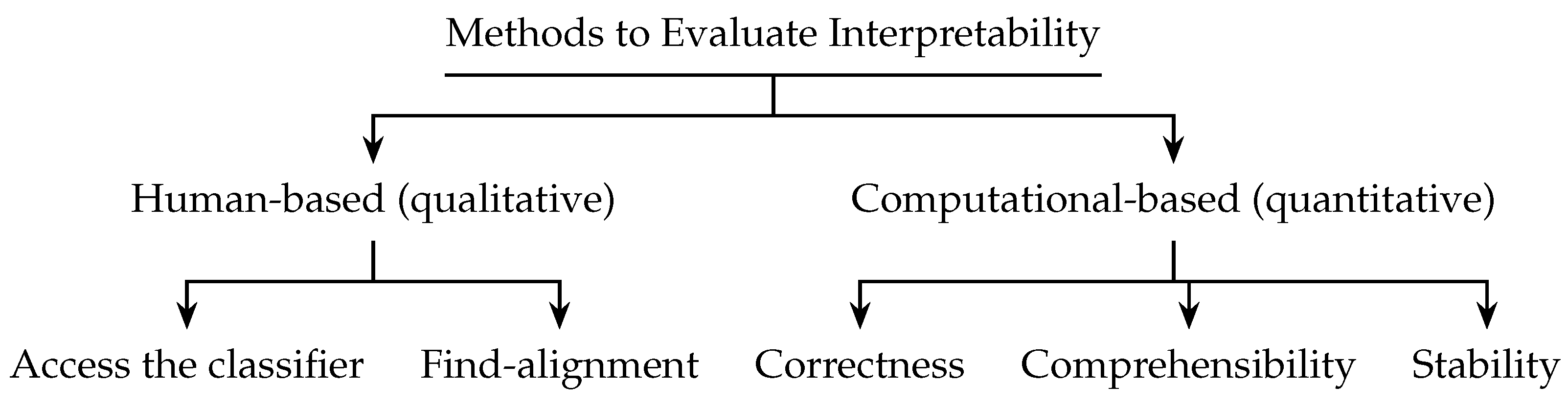
• Fidelity: Does the resulting explanation accurately reflect the computation performed by the original model during the decision-making process? To prevent providing a falsely convincing explanation, the reported explanation must be faithful to what is computed. Generally, unfaithfulness is brought up in post hoc explanations. In this survey, we group all methods that examine this factor under the heading “evaluating correctness”. Additionally, instability is an undesirable phenomenon that undermines our trust in the model’s decision; thus, a further subsection is introduced to examine the robustness of the interpretation.
• Comprehensibility: Are the generated explanations “human-understandable”? This can be determined by designing an experiment in which human assessors judge the understandability or by relying on the findings of prior research that have demonstrated the understandability of a particular model, such as a rule or tree. This factor is discussed in two subsections of this survey: human evaluators and comprehensibility.

Existing surveys on interpretable machine learning, such as [5,8,14,17], primarily concentrate on presenting and categorizing various proposed approaches. However, they often do not extensively discuss the assessments of these approaches. While some surveys include a section on evaluation aspects, they may not be comprehensive [18]. Additionally, certain surveys specifically center on the evaluation of causal interpretability, like the work by Moraffah et al. [19]. To address this gap, our survey primarily emphasizes the evaluation of feature-based methods. These methods, recognized for their simplicity and intuitiveness, have been extensively studied and benchmarked among the various approaches for providing interpretations [20].

This survey categorizes the literature on evaluating interpretability into qualitative and quantitative evaluations (Figure 2), with the former relying on humans and the latter employing computational metrics to evaluate correctness (fidelity), comprehensibility (providing the interpretation in human-understandable terms), and robustness (stability). It provides insights into the existing interpretability evaluation methods to understand each method’s suitable scenario.

The rest of the paper is organized as follows. The background section covers the fundamental concept in the domain required to go through in the paper. The qualitative evaluation section (human-based) reviews human-subject studies to assess interpretability. The quantitative evaluation section reviews existing computational methods and is separated into three subsections: fidelity, comprehensibility, and stability. Finally, a discussion of the findings and conclusions is presented.

2. Background

When studying the interpretability of predictive models, we may choose to consider a set of dimensions which determine the model’s interpretability.

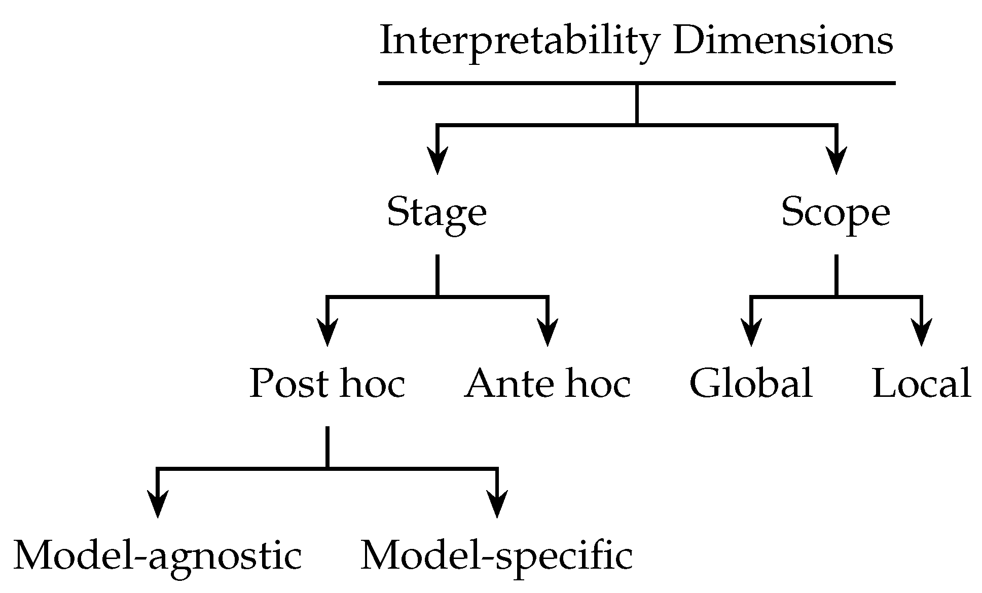
2.1. Interpretability as Stages: Post Hoc vs. Ante Hoc

Explaining a machine learning model can be achieved by either adopting a transparent model (using an inherently interpretable model such as a decision tree or injecting the interpretation with the learning process to enable the model to generate explanations in the process of decision making) (intrinsic or ante hoc) or by interpreting the model after its completion process (post hoc) [8]. The post hoc requires extra modeling effort. Its main advantage is the preservation of accuracy, and it can be used with already-existing models. In intrinsically interpretable models, in some cases, the interpretability comes at the cost of accuracy.

Post Hoc Interpretability

Post hoc interpretability has two main categories: model-agnostic and model-specific. Agnostic approaches are not tied to any particular type of black-boxes nor do they require the original data to provide their explanation. Usually, model-agnostic approaches utilize reverse engineering to acquire the approximation of the original model as they are only able to observe the input and output of the black-box model. Thus, the black-box is queried with a test dataset in order to create an oracle dataset to train the explainer and operate on data level only without accessing the inner details of the model. Model-agnostic interpretability becomes the only choice when we try to explain proprietary models and also discover the pattern in the model’s behavior. Model-agnostic approaches vary from simple, such as partial dependency plot PDP, to complex, such as SHAP [21], which is a game-theoretic technique based on Shapley values. Model-specific approaches, on the other hand, consider input, output, and the inner-workings of the model. So, they are tied to a particular type of black-box and cannot be generalized to other types.

2.2. Interpretability by Scope

In global interpretability, the model is completely interpretable, and we can understand the model’s logic and the reasoning behind different possible outcomes. TERPAN [22,23] is an example of global interpretation that fits a black-box into a simpler model.

In local interpretability, the interpretation does not explain the whole model’s behavior but instead it is provided per decision. Many approaches provide local interpretation, either by locally approximating the complex model around the point of interest or by providing the most important features in different forms (heat maps for images [24,25], weight of features [1], etc.). For example, a perturbation-based approach queries the model with perturbed versions around the point of interest to approximate the model locally; Local Interpretable Model-Agnostic Explanations (LIME) [1] is an example of this approach.

The saliency/heat maps are another form of local explanation to explain the prediction of neural networks. They present the explanation visually by highlighting the most influential parts in the input. The salient regions could be identified by deleting or “perturbing” different regions, then observing how the prediction changes [26]. The network is repeatedly tested to produce a heat-map that highlights the most influential parts of the data [27]. A saliency map can be computed directly using the input gradient; it gives importance weights to pixels based on first-order derivatives [28]. As the derivatives can miss important aspects of the information that flows through a network, other enhanced approaches have been proposed, such as class activation mapping (CAM) [24] and gradient-weighted class activation mapping (Grad-CAM) [25]. These maps are useful to give insight on the most influential parts, or where the network is looking. However, they are restricted to neural networks (mostly CNN), and some times they are scattered and need to be interpreted.

These dimensions may overlap as one model can be post hoc and either local or global. Some examples include LIME [1], which is local, post hoc, and model-agnostic, and GoldenEye [29], which is global, post hoc, and model-agnostic. However, no overlap can be found between intrinsic and agnostic models.

Another rarely mentioned dimension is the output type, which is the dimension with the least overlap. Regardless of whether the interpretation is local or global, it may be expressed in terms of features such as the weight of the most affected feature or salience features, another instance to explain the prediction (prototype, critic, counterfactual, influential training example), or another model (simpler model). The feature-based interpretation is provided as the attribution of each feature, or, in other words, a ranking of which features mattered most to the model in making a prediction for the given instance or for the whole model. The attribution can be found either by perturbing input instances around the point of interest, then approximating the decision boundary of the original model using perturbation-based methods, or by calculating the partial derivative of the target with respect to every input feature using gradient-based methods. In the instance-based interpretation, it is provided as an example that could be prototype, critic, or counterfactual. In the first one, the prototype interpretation provides representative points for the class, while influential examples are provided by looking at the training examples and finding the most influential one to model prediction for the point of interest. Meanwhile, the counterfactual interpretation provides the required change for the point of interest to flip the prediction.

3. Qualitative Evaluation: Human-Based

Human assessment is essential for evaluating interpretability [7]. However, human-subject experiments should be well designed to meet the required goals, such as simulatability and decomposability. This section aims to survey and categorize the different human-based tasks to evaluate interpretability. The different tasks in the literature have two main goals: assess the explanation’s ability to grant the user access to the classifier logic and find the alignment between the human and classifier logics (see

Table 1. Qualitative evaluation.

	Lay	Expert	Lay + Expert
Specific	- Understand internal reasoning process [30] - Reconstruct target instance [31]
All models	- Verification [32,33] - Counterfactual [32]	- Alignment between human and model  [21,34,35]	- Forward Simulation [6,7,30,32,36,37,38,39] - Select the best explanation  [7,21,26,30,36,40,41,42] - Describe the class characteristics  [43,44]
Agnostic	- Select the best classifier [1,25,45,46] - Improve a classifier [1] - Alignment between human and model [46,47]	- Identify classifier irregularities [1]

).

3.1. Access the Classifier

In this category, tasks are designed to assess whether the interpretation provides sufficient information to understand the classifier’s logic.

Task 1: Select the best classifier

Can human subjects select the best classifier based on the explanation alone? By presenting explanations of two different classifiers along with their corresponding data, the user is then prompted to choose which classifier performed best. In both [1,45], providing explanations helped the user determine the best classifier.

Similarly, in [25], when conducting the same task, users were able to select the more accurate classifier based on prediction explanations, despite the fact that both models made identical predictions on the presented subset of instances. Kim et al. [46] term this activity the “distinction task”. In this task, they present four predictions along with their respective explanations for a given input image. Participants are then asked to identify the accurate prediction based on the provided explanations. This “distinction task” also serves to alleviate the impact of confirmation bias in interpretability assessment, as participants must now consider multiple explanations concurrently.

Task 2: Improve a classifier

Can human subjects improve a classifier (by performing feature engineering) based on explanations only? In this task, an instance with its explanation is presented to a non-expert user, and the user has to enhance the classifier by identifying which feature should be removed from subsequent training [1]. As mentioned, users are non-experts and have no access to data, so the identification is made solely based on the explanation content. However, the users were able to identify and remove the unimportant features from the task. Across rounds, the users converged to the same ‘correct’ model. This high agreement is evidence of the ability of the explanation to improve the untrusted classifier.

Unlike the common concept of the trade-off between accuracy/interpretability tasks 1 and 2, accuracy and interpretability are not necessarily opposite concepts but can be positively correlated; as we see here, interpretations improve accuracy.

Task 3: Identify classifier irregularities

Can human subjects identify and describe classifier irregularities based on the explanation only (insights)? During training, the artifacts in the data lead to undesirable correlations. Therefore, can explanations reveal this correlation? To answer this question, a logistic regression classifier is trained to distinguish between photos of wolves and huskies based on snow in the background [1]. The experiment starts by showing test predictions that are all correct except one, without explanation to an expert. Then, the expert is asked questions (Do you trust the algorithm? Why? How do you think this algorithm distinguishes between images?). After that, an explanation is shown, and the same questions are repeated. By comparing the answers before and after explanations, more than 30% answered yes to “do you trust the classifier?”, and less than 50% noticed the snow in the background. After presenting the explanation, all experts obtained the correct insight, and the trust decreased.

Task 4: Forward Simulation

Can human subjects correctly predict outcomes based on explanations only “forward simulation/prediction”? Doshi-Velez and Kim [7] suggested “forward simulation/prediction” as an evaluation approach of interpretable models. In this approach, both an explanation and input are presented, and the user is asked to predict the model’s output, i.e., the user is asked to simulate the model’s behavior based on the explanation. Forward simulation is used frequently in assessing interpretability, as in [36], where the users were asked to predict the classifier behavior on a random set with binary forced choice.

A short survey is presented to users with backgrounds in machine learning to make predictions on given instances in [37]. The mean response time is used to estimate interpretability in [38] after the user is provided with a list of feature values along with a graphical depiction of the explanation, and then the user is asked to make a prediction. An important finding is that using the same users across all experiments substantially reduced response time, which is one of the most vital shortcomings of using humans to compare among different models.

A simulation was also used in [30,39] to evaluate how well the user understood the model process.

An empirical study of the complexity factors most affecting human simulatability is presented in [32]. This study was conducted by varying three types of complexity model sizes, cognitive chunks, and repeated terms. Three metrics were considered to measure the effect response time, accuracy, and subjective difficulty. The simulation task was studied by varying the number of cognitive chunks between 1, 3, and 5. Unsurprisingly, increasing the complexity results in longer response times, especially for cognitive chunks, while the other two metrics were less clear with varying cognitive chunks.

Task 5: Counterfactual

Can human subjects determine if the correctness of a prediction would change if some of the features in the input example were changed? In this task [32], the users were asked to change features in the input data, which led to a change in the model’s prediction. This task aims to determine whether the users are able to detect how to change the prediction by making small changes in the input.

Task 6: Describe the class characteristics

Can human subjects describe all the characteristics of a class based on the explanation? To determine the human ability to understand the decision boundaries of the classes in the data along with the classes’ patterns, this task [43] was carried out in two stages: descriptive questions and multiple choice questions. In the first stage, the users were asked to explain in plain text all the characteristics of a particular class based on the explained model (the presented rules). In the second stage, the users were asked “true” or “false” questions to decide if the information provided was sufficient to conclude a particular class.

The same approach was followed to assess the human understandability of an extracted tree [44] by asking the user to determine how the interpretable model (tree in their case) classifies a given instance, and whether the user is able to select a subset of features with a relevant one.

3.2. Find Alignment

In this category, the tasks were designed to evaluate how close the explanation is to human reasoning.

Task 7: Alignment between humans and models

Are the human explanations aligned with the one provided by the model? Based on the idea that a good model explanation should be consistent with humans’ explanation. Model comparison is performed among LIME [1], DeepLIFT [48], and SHAP [21] with human explanations. Human subjects were asked to write a short description; then, agreement between human explanations and the explanations of the other three models was identified [21]. However, the match between human and model explanations does not imply explanation correctness, especially if all the used models are post hoc.

On the assumption that alignment implies consistency, the authors of [34] propose a measure for “human accuracy” that evaluates the alignment between the labels provided by humans for certain terms corresponding to and those produced by the model.

The most basic approach of evaluating extracted reasonings is comparing them to human-marked reasonings. Evaluating Rationales and Simple English Reasoning (ERASER) [35] is proposed as a benchmark with exhaustive annotated rationales for NLP tasks, along with two types of metrics: exact matches and ranking metrics. The amount of overlap between the ground truth and the extracted reasonings in an exact match case is calculated using the intersection-over-union (IOU) measure, a metric derived from computer vision that allows partial match credit assignment. In the ranking cases, marked tokens receive higher points. Specifically, the area under the precision-recall curve (AUPRC) is calculated by moving a threshold over the token scores.

Yang et al. [47] refer to this task as “groundability”, which measures the alignment of model interpretations with human interpretations.

Kim et al. [46] refer to this task as the “agreement task”. They sequentially provide participants with individual prediction–explanation pairs and inquire about their level of confidence in the model’s prediction based on the explanation. This task gauges the extent of confirmation bias stemming from a specific interpretability method. Nonetheless, it does not assess the effectiveness of explanations in discerning accurate from erroneous predictions—an essential aspect of explanations in AI-assisted decision-making.

Task 8: Select the best explanation

Human subjects are given two different explanations from two different algorithms and select the one that they find to be of better quality. This approach is presented in [7] as a binary forced choice and is the most commonly used approach in the literature [21,26,30,36,40,41,42].

Task 9: Verification

Can human subjects find consistency between system prediction and recommended prediction? In this task [32,33], the user is given observations (data instances), predictions recommended by the model, and an explanation, and then, the user decides based on the explanation of their agreement/disagreement with the recommendation.

Task 10: Understand internal reasoning processes

Can human subjects understand the internal reasoning process by showing the visualization of the model’s intermediate outputs at each step? In this task [30], users were shown the model’s intermediate outputs along with the final prediction and then asked to judge whether they understood the internal reasoning process or what the model was doing at each step.

Task 11: Reconstruct target instance

Can human subjects reconstruct target instance by modifying each component of the generative model? In this task [31], a user is presented with two representation values, z and $z^{\prime }$, along with their respective instance values, x and $x^{\prime }$, as well as the distance between them, $d(x,x^{\prime })$. Additionally, they give controls (sliders for continuous dimensions, radio buttons for discrete dimensions) that let the user to alter each component of z. This quantifies the human interpretability of generative model representations and is referred to as “interactive reconstruction”.

3.3. Discussion

Qualitative evaluation is useful for providing insight into how humans react and for understanding the interpretation/explanation provided by the model. Lakkaraju et al. [43] utilized human users because they believe that “there can be no better judges than humans to evaluate this notion of interpretability”. However, many factors can influence the results of human experiments, such as human fatigue, inadmissible practice sessions, and human background. Furthermore, studies have shown that humans trust and are satisfied with a model’s explanation if it matches their expectations and their point of view. Therefore, relying on human trust as an evaluation metric is a source of bias, as such a metric rewards the alignment and similarity instead of faithfulness and correctness [49]. Also, providing explanations increases human trust regardless of its correctness, Kim et al. [46] found that providing explanations makes participants more likely to believe that the model predictions are correct. For example, 60% of their participants found the explanations for incorrect model predictions convincing, which aligns with the observations of Poursabzi-Sangdeh et al. [50].

Herman [49] states that considering cognitive attributes and user expectations as indicators for user trust and understanding introduces bias, causing implicit human cognitive bias. Finally, as demonstrated in [51], a model may provide plausible but poorly faithful explanations.

An important consideration with human-based tasks is to ensure that participants rely on the provided explanations rather than their existing knowledge to complete the task. This phenomenon is often referred to as the “effect of human prior knowledge”. To mitigate this effect, Kim et al. [46] adopted several measures, including selecting non-common contexts that are not readily known by non-experts and omitting semantic class labels.

Also all the reviewed papers have one common aspect: human-based evaluations are consistently conducted on relatively small sample sizes. The largest of these studies was undertaken by Kim et al. [46], involving 1000 participants.

4. Computational Metric: Correctness with Respect to the Original Model/Faithfulness/Fidelity

One of the most important criteria in assessing an interpretation is its correctness with respect to a black-box model (the model being explained). Correctness, often referred to as faithfulness or fidelity, assesses “the ability of the explanations to reflect the behavior of the prediction model” [52]. Depending on the nature of explanation, many approaches are employed to determine fidelity (see

Table 2. Explanation correctness approaches.

References	Validation Approach	Explanation Type
[22,44,53,54]	Separate test-set	Global models (post hoc)
[43,55]	Ablation studies	Global models (intrinsic)
[34,40,41,48,56,57,58,59,60,61,62,63,64,65,66,67,68,69,70,71,71]	Removal-approach	All feature attribution approaches
[35,55,61,72,73,74,75]	Compare interpretation with ground-truth	All types when data are available

).

4.1. Interpretation as Model

In this category, the original model is approximated by a simpler proxy model (post hoc) or the interpretation is augmented during the model building process (ante hoc/intrinsic). The first consideration is how well the approximation matches the original model. Fidelity ensures that the proxy model captures the decision-making process of the original black-box model, so the explanations are accurate and can be used to understand the target model (

Table 3. Explanation correctness of models.

Ref.	Metric Name	Proxy Model	How the Faithfulness Measured
[22]	Fidelity	Decision tree	The percentage of test-set examples on which the classification made by a tree agrees with black-box (NN) counterpart.
[53]	Fidelity	Linear model,  iGAM	Compare the output of both black-box with transparent models on test-sets
[44]	Accuracy relative to the complex model	Decision tree	Find the match between the two models on test-sets
[55]	-	Global prototypes per class	Use prototypes in nearest-prototype classifier

summarizes the various techniques).

TREPAN [22] ensures that the extracted tree accurately models the networks by measuring the percentage of agreement between the tree and network on test-set examples. The same procedure was followed in [53] by considering the black-box models as teachers, while the student was the transparent model that mimicked the scores assigned by the teacher. Then, how accurately the student models anticipated their teachers’ outputs was examined on test sets. Additionally, in [44], the decision tree extracted from a random forest was evaluated on a separate test set to see how well its predictions matched those of the random forest. The test was based on the F1 score, and a close match implies the faithfulness of the interpretation. In line with the idea of evaluating explanations on independent test sets, Tan et al. [54] evaluated the selected prototypes by using them in another model nearest-prototype classifier. They interpreted tree ensembles by providing different numbers of prototypes for each class.

Ablation studies aim to determine the effect of different components of the objective function by removing one objective and observing the result. In [43], ablation studies are used to ensure the correctness of decision sets by studying the impact of removing different components from the objective function on the interpretability and predictive accuracy. At each time, one objective is removed, the precision, recall, and overlap, the predictive power and interpretability of these ablated models are quantitatively evaluated. Additionally, in [55], ablation studies are used to assess the different components of their generative model.

Self-Explaining Neural Networks (SENN) [76] provide an intrinsic explanation by teaching the neural network to explain itself. To provide interpretations, the SENN model relies on the basis concepts. Individual features in low dimensions, tissue ruggedness, or irregularities in image processing are examples of basis concepts that are either learnt by a network or offered by an expert. When SENN classifies any instances, it assigns relevance scores (weights) to each of the basis concepts. Consequently, in this context, fidelity assesses how closely the relevance scores correspond to truly relevant features. To address this question, researchers analyze how deleting features affects the model’s prediction. First, some features were removed, the decrease in the probability of the predicted class was measured, and the prediction of the model was compared against the interpreter’s own prediction of relevance. After that, the correlation of these probabilities decreases and the relevance scores on various points were computed, and the aggregate statistics were shown.

Global fidelity is not always attainable. Hence, proxy model local fidelity has been introduced in LIME [1], where fidelity corresponds to the model behavior with respect to the instance being explained. Global fidelity implies local fidelity, but local fidelity does not entail global fidelity. LIME approximates the model locally using a simpler model and relies on qualitative evaluation; LIME only codifies fidelity but never quantifies it.

4.2. Interpretation as Feature-Attribution (Saliency/Heat-Maps)

Interpretation can be provided in terms of the most contributed/important features for a given decision. Across a variety of fields, feature importance was by far the most used and studied interpretability approach [20]. Often, it is referred to as feature-level interpretation, feature attribution, feature contribution, or saliency map. Depending on the input, important features might be coefficient weights, saliency maps that assign a weight to each pixel based on its importance, or the most significant words in natural language processing (NLP).

This method’s flaw is that it provides interpretations in input terms, which usually seem persuasive but are not always accurate. For instance, saliency methods highlight the pixels that best represent the real class in the image. They primarily determine where the classifier “looks” to produce a prediction. They are popular in explaining the prediction of deep neural networks on images. As revealed by sanity checks [56], depending solely on visual assessment might be deceiving. Sanity checks [56] evaluate the adequacy of explanation approaches based on the concept of a statistical randomization test, which compares a natural experiment against an artificially randomized experiment. Two randomized tests were investigated: a model parameter randomization test and a data randomization test. The first test is a model parameter randomization test, where the output of a saliency method performed on a trained model is compared with the output of the same model architecture with random weights. If the saliency method relies on the model’s parameters, then the output of the two cases should be different. While the similarity of the outputs indicates the insensitivity of the saliency map to the model parameters, saliency is not useful in understanding the model’s behavior. The second test is a data randomization test, where the saliency method performed on a base model is compared with the output of the same model trained with randomly permuted labels. If the saliency method relies on the data labels, the output of the two cases should be different. The insensitivity indicates that the method does not depend on the relationship between the instances being explained and their class labels. However, some tested methods fail the proposed tests and are invariant to either network reparameterizations or label perturbations. Thus, the failed methods are inadequate for some tasks, such as model debugging.

Evaluating the saliency map correctness had to ensure that the highlighted pixels are the actual pixels used during classification (relevancy of the heat map). The quality of the saliency map depends on the quality of both the algorithm used to compute it and the classifier’s performance. Thus, it is very difficult to define objective criteria.

Many approaches suggested in the literature include removal-based and ground-truth approaches. In the removal-based approach, input variables that are highly important for the prediction are perturbed or masked to determine whether this causes a decline in the prediction score or in the expected difference between input explanations when applying perturbations to the output (see

Table 4. Correctness of feature attribution (Perturbation-approach).

Ref.	Metric Name	Removal	Approaches
[56]	Fidelity	Remove	Measure the drop in probability after the perturbation
[57]	Faithfulness	Replace by baseline values	Find subset features perturbation to a baseline
[58]	Explanation  selectivity	Remove	Measure the drop in probability after remove important feature
[40]	AOPC	Remove	The same as [58], on patch of size 9 × 9
[59] [60]	-	Replace by random sample from uniform distribution	Same as [58]
[61]	AOPC	Remove	Extended AOPC to evaluate negative attributions to irrelevant regions
[62]	-	Replacing with zero	Same as [40], one pixel at a time
[41]	(CPP) and  (NLCI)	Replace positive by 0,   and negative by 1.	Find the change of prediction probability and the number of label-changed instance
[63]	Pixels flipping	Flip the pixels	Change pixels with highly scores then evaluate the effect
[64]	-	Iterative removal	Remove the segment with highly score then, find the drop in AOC
[48]	-	Required change to flip the class (erase)	Find log-odds score change between original image and perturbed image in another class
[65]	Completeness	Baseline	Sum of features’ attribution should sum up to difference in prediction wrt baseline
[62]	Sensitivity-n	Baseline	Quantify the attributions difference when remove a subset of features
[66]	Infidelity	Baseline, noisy baseline,  and multiple baselines	Same as [62], with different perturbations
[67]	-	Remove	Re-train models on the perturbed instances before find the drop
[68]	-	Remove features  one-by-one	Find the differences and correlation
[34]	Post hoc accuracy	Zero padding	Compute accuracy level between original and padded instance
[69,70]	Precision and   recall	Masking with uninformative from original distribution	Utilize AUP and AUR
[71]	Saliency metric	Cropping relevant region	Utilize entropy to validate the classifier ability to recognize class

). In the ground truth approach, the areas located on saliency maps are compared to annotated data.

4.2.1. Removal-Based Evaluation

Three phases can be used to organize methods for validating feature-based interpretations.

• Select features to remove, either randomly or based on their importance.
• Fill in the blanks of features, and this is where the methods vary (either filling the blank with the background, or replacing it with the mean, or ignoring it, etc.)
• Calculating the difference between the presence and absence of a feature to determine its predictive impact (reporting the decline in accuracy relative to the trained model).

Bhatt et al. [58] quantified the faithfulness of feature attribution by setting a particular feature $x_s$, where s refers to a randomly selected feature subset $\left|S\right|$ and replace those features with baseline values $\overline{x_s}$. Then, they measure the correlation between the sum of attribution of $x_s$ and the difference in output when replacing s with baseline (see Equation (1)). If the change in output is proportional to the sum of attribution scores of the features in $x_s$, then the explanation is faithful.

$${\mu }_F(f,g;x)=\underset{s\in \left(\genfrac{}{}{0pt}{}{\left[d\right]}{\left|s\right|}\right)}{\mathrm{corr}}\left(\sum _{i\in s}g{\left(f,x\right)}_i,f\left(x\right)-f\left(x_{[x_s=\overline{x_s}]}\right)\right).$$

(1)

In Equation (1), corr is Pearson’s correlation, f is the predictor, g is the explanation function, d is the total features, s is the randomly selected subset of features, and x is the point of interest. However, the accurate estimate of all $\left(\genfrac{}{}{0pt}{}{\left[d\right]}{\left|s\right|}\right)$ subsets may not be obtained and it is even harder to aggregate.

The same approach was followed in [68] on Gaussian process regression. The features are removed one-by-one to find the differences between the predictions made with the original input and the perturbed input. Then, the correlation between the differences and the contributions of the removed features are calculated.

Saliency methods assign a score to each input variable, which is utilized to evaluate the fidelity of the explanation. In [57], the scores are sorted from most to least significant, and the related input variables are eliminated iteratively, beginning with the most significant, to track the prediction value by making a plot and finding the area under the curve (AUC). A sharp drop in the function value (low AUC score) is an indication of fidelity. The same approach was followed in [40] on patches of size 9 × 9 to measure the Area Over the most relevant first Perturbation Curve (AOPC). Ordering regions according to importance implies a steep decrease in the graph of Most Relevant First (MoRF) and thus a larger AOPC. In [59,60], the highly important values in the input were replaced by random samples from a uniform distribution.

Instead of using a 9 × 9 patch, Ancona et al. [62] operate at the pixel level by replacing one pixel at a time with a zero value and then measuring the change. This metric was extended to evaluate the distribution of the negative attributions to the irrelevant regions of the prediction by perturbing the Least Relevant First (LeRF) and then finding a decrease in the accuracy [61].

Based on the same assumption that a good interpretation model should identify the most relevant features to the predictions, Cong et al. [41] evaluated the effectiveness of their feature attribution by sorting the absolute weights of the input features in descending order. Then, the input features (positive weights with 0; negative weights with 1) were iteratively altered one at a time for up to 200 features. Then, two metrics were used in the evaluation: the change in prediction probability (CPP) and the number of label-changed instances (NLCI). CPP is the absolute change in the classifying probability, and NLCI is the number of instances whose predicted labels change after the alteration.

Pixel flipping is also used in [63], by change pixels with highly positive and highly negative scores and then evaluates the effect of flipping on the prediction scores.

To minimize the computational cost, the Iterative Removal Of Features (IROF) was proposed [64]. Each image is partitioned into a set of segments; then, for each segment, the mean importance is found, and then, the segments are sorted in decreasing order of importance score (relevance). A high-relevance-score segment is removed, and the class label is found. Finally, the area over the curve (AOC) is computed for the class score. A high AOC is an indication of the goodness of the explanation method.

The completeness axiom [65] states that the sum of the attributions equals the difference between the output of F at instance x and baseline $x^{\prime }$, where $x^{\prime }$ is set to be a black image (zero attribution). $F:R^n\to R$ is differentiable almost everywhere, so

$$\sum _{i=1}^n{\mathrm{attribution}}_i\left(x\right)=F\left(x\right)-F\left(x^{\prime }\right).$$

(2)

An extension of the completeness axiom is sensitivity-n [62], which requires that attributions of a subset of features of cardinality n sum to the difference between the value of F at instance x and baseline $x^{\prime }$; completeness is achieved when n is equal to the total number of input features.

More general perturbations than setting the feature values to 0 or a baseline have been investigated in [66]. Perturbations can be the difference from the baseline, or a subset of differences from the baseline, or the difference from a noisy baseline, or the difference from multiple baselines. Then, the infidelity is measured by:

$$INFD(g,f,x)={\mathbb{E}}_{I\sim {\mu }_I}\left[{\left(I^{T}g(f,x)-f(x-I)\right)}^2\right],$$

(3)

where, f: a black-box function, g: explanation functional, x: a random variable with probability measure ${\mu }_I$, $I=x-x_0$ is the difference to the baseline. Chih-Kuan et al. [66] found that many existing explanations are optimizing the infidelity with respect to various perturbations.

Shrikumar et al. [48] designed a task to evaluate different feature attribution methods. The task starts by selecting an image that originally belongs to class $C_o$, erasing pixels (up to 20%) in a way that converts the image to another target class $C_t$ and then finding the score as follows:

$$S_{x_i\mathrm{diff}}=S_{x_i{C}_o}-S_{x_i{C}_t},$$

(4)

where $S_{x_i}$ is the score for pixel $x_i$ and class c. Sort images in a descending order according to $S_{x_i\mathrm{diff}}$, to evaluate log-odds score change between each of $C_o$ and $C_t$ for the original and perturbed images.

Instances where the features are removed or perturbed come from a different distribution, which violates the assumption that states that the training and evaluation data must come from the same distribution. As a result, the degradation in model performance could be due to the distribution shift. To overcome this problem, RemOve and Retrain (ROAR) [67] retrain models on the perturbed instances so that both training and test data come from the same distribution. However, the resulting model after retraining can be slightly different than the original model. Also, repeating the retraining process multiple times to lower the accuracy variation is computationally costly. Notably, a similar approach is also adopted by Meng et al. [77].

L2X [34] selects the most informative features for a given instance. L2X maximizes the mutual information between the subset of feature $x_s$ and response y through the selector E. In particular, it optimizes the criterion: $maxI(X_S;Y)$ subject to $S\sim E\left(X\right)$. In order to validate the effectiveness of their method, they introduced post hoc accuracy by feeding sample X to the model after masking the unselected features with zero padding. Then compute the accuracy using $P\left(y\right|X_s)$ to predict samples in the test dataset labeled by $P\left(y\right|X)$. Masking the correct salient features results in a steep decline in accuracy, showing that the removed feature is necessary for accurate prediction. When irrelevant features are removed, the accuracy level remains intact. However, the unaltered outcome may also occur if the removed feature is essential but insufficient to cause the model to behave incorrectly. As a result, Ismail et al. [69] advise against basing comparisons of saliency methods solely on the loss of accuracy after masking. Instead, the features should satisfy the following two criteria: all identified salient features should be informative (precision), and the saliency method should be able to identify them (recall). In evaluating time series data, they thus utilized the area under the precision curve (AUP), the area under the recall curve (AUR), and the area under the precision and recall curves (AUPR). Using the accuracy and recall values at various levels of deterioration, the curves are computed after masking the features with uninformative ones from the original distribution. The same approach is adopted in [70].

The goal of instance-wise feature selection is to select from the ith instance $x^i$ the minimum subset of features $x_{s^i}^i$ satisfying: $F\left(y\right|x_{s^i}=x_{s^i}^i)=F\left(y\right|x=x^i)$ with regard to the target y [78]. The problem is ensuring that both points belong to the same distribution. For that purpose an evaluator model EVAL_X [78] is trained to evaluate the selected features on true conditional distribution. The subset of features represented by a binary vector, however, is selected at random, independent of x, from a Bernoulli distribution, which resembles any potential input selection. In practice, optimality may be difficult to achieve because there are $2^d$ different combinations. In addition, since the evaluator model is different from the original model, explanation metrics computed using this evaluator model may not accurately reflect the fidelity of explanations.

Alangari et al. [79] introduced both global and local fidelity metrics for Gaussian Mixture Model. For global validation of feature importance, they marginalized the contribution over that specific feature. On a local level, they employed two metrics comprehensiveness and sufficiency. Comprehensiveness, which mandates the inclusion of all contributing features. Excluding these features diminishes the model’s confidence.

$$\begin{array}{c}\hfill {\mathrm{comprehensiveness}}_k=P\left(C_k\right|x^D)-P\left(C_k\right|x^{D-S}),\end{array}$$

(5)

where, $D=\{f_1,\dots ,f_d\}$ full set of features, x instance being explained, $C_k$ is the kth cluster, S is the selected subset of features as class evidence and D is the full features.

Sufficiency, which seeks the subset of features that, when retained, sustains or boosts the model’s confidence.

$$\begin{array}{c}\hfill {\mathrm{sufficiency}}_k=P\left(C_k\right|x^S)-P\left(C_k\right|x^D).\end{array}$$

(6)

4.2.2. Entropy-Based Evaluation

In addition to masking and perturbing the highly important features, Dabkowski et al. [71] suggested locating the tightest rectangular crop that includes all the salient or important regions and then feeding it back to the classifier to validate its ability to recognize the requested class. A correct saliency method will minimize the crop size without affecting the classification probability p. This metric is referred to as the saliency metric, which is measured by the following formula [71]:

$$s(a,p)=log\left(\tilde{a}\right)-log\left(p\right),$$

(7)

where $\tilde{a}=max(a,0.05)$, a is the area of the rectangular crop/the total image size, and p is the probability of the requested class returned by the classifier based on the cropped region, where a low value of s is an indication of good saliency detectors. However, cropping images results in images with arbitrary sizes, and not all classifiers accept this; thus, this metric works with classifiers that are invariant to scale and aspect ratio.

4.2.3. Compare Interpretation with a Ground-Truth

With prior knowledge of feature importance, the salient features are compared to the ground truth. Table 5 presents some of the used datasets. Ground truth fidelity is defined by Dai et al. [75] as the intersection of the top k features of the ground truth and the explanation, divided by k.

The availability of bounding box annotation is utilized in [72] to assess the positive relevance scores in the heat map by computing the outside–inside relevance ratio metric $\phi$ as follows:

$$\phi =\frac{\frac{1}{P_{out}}{\sum }_{q\in P_{out}}{R}_q^{\left(1\right)}}{\frac{1}{P_{in}}{\sum }_{p\in P_{in}}{R}_p^{\left(1\right)}},$$

(8)

with $|.|$: the cardinality operator, and ($P_{out}$ and $P_{in}$): set of pixels outside and inside the bounding box, $R_i^{\left(1\right)}$ is the relevance value attributed to the ith computation unit at the first layer.

The outside–inside relevance ratio metric $\phi$ is extended in [61] to simultaneously evaluate both positive and negative relevance scores.

$$\phi =\frac{\frac{1}{P_{out}}{\sum }_{q\in P_{out}}{R}_q^{\left(0\right)+}+\frac{1}{P_{in}}{\sum }_{p\in P_{in}}{R}_p^{\left(0\right)-}}{\frac{1}{P_{in}}{\sum }_{p\in P_{in}}{R}_p^{\left(0\right)+}+\frac{1}{P_{out}}{\sum }_{q\in P_{out}}{R}_q^{\left(0\right)-}},$$

(9)

$R_i^l$ is relevance of a neuiron i in a layer l.

Additionally, Nam et al. [61] utilize segmentation masks and metrics to overcome the nonperfect fit of the bounding box for the object corresponding to the prediction. Normalized cross correlation (NCC) [55,73] is used to compare the saliency absolute values of the attribution and the ground truth masks.

Feature attribution and interaction scores are evaluated by Tsang et al. in [80] against the ground truth of annotation labels on subsets of features. Moreover, Tsang et al. [80] compare their model performance in three tasks (sentiment analysis, image classification, and recommendation) with that of state-of-the-art models. In the sentiment analysis task, they use two metrics: phrase correlation and word correlation. In image classification, they compare their model to state-of-the-art methods by computing the agreement between the estimated attribution of an image segment and that segment’s label “Segment AUC” metric. Due to the absence of ground truth annotations in the recommendation task, only positive feature interactions are considered.

Ying et al. [74] prepared synthetic datasets with ground-truth explanations and then used them to calculate explanation accuracy. As [74] aimed to interpret graph neural networks, they formalized the explanation problem as a binary classification task, where the edges are the labels and the explanation methods’ importance scores are the prediction scores. A higher score for edges is an indication of a good explanation method.

ERASER [35] is a benchmark that consists of numerous NLP datasets and tasks for which human annotations of “reasonings” have been gathered, as well as a number of metrics designed to measure how well the rationales produced by models correlate with human rationales and how faithful these rationales are. To prevent plausible interpretations, two metrics, comprehensiveness and sufficiency, are designed to capture faithfulness. The first metric, comprehensiveness, indicates if all the features required to make a prediction were selected. The sufficiency metric should indicate whether the extracted reasonings include sufficient information to make a decision. To determine comprehensiveness, take input instance $x_i$, eliminate reasoning $r_i$ to generate $x_i^{\prime }$, and then feed both $x_i$ and $x_i^{\prime }$ into model F to find the difference. A large difference indicates that $r_i$ did indeed affect the prediction and lower the model confidence. The purpose of sufficiency is to determine if the extracted reasonings are adequate for making a prediction. Thus, $x_i$ and $r_i$ are both input into the model, which calculates the difference to decide if retaining features would improve or preserve the model’s confidence. The same metrics were employed in [81] to compare five feature removal approaches in NLP tasks.

Ribeiro et al. [82] have introduced the STructured REasoning and Explanation Multi-Task benchmark (STREET), which comprises a range of NLP question-answering tasks encompassing quantitative, analytical, and deductive reasoning. This dataset is constructed by augmenting five existing QA datasets through the addition of reasoning graphs as annotations to the answers. The objective for models using this benchmark is to generate an answer accompanied by a reasoning graph that provides an explanation for the answer. Two metrics are employed to evaluate the reasoning graph. The first metric is Reasoning Graph Accuracy, which involves comparing the predicted reasoning graph with the golden reasoning graph, considering both the graph structure and the content of the intermediate conclusion nodes. It is important to note that this metric is strict, and even slight deviations from the golden reasoning graph would deem the predicted graph as incorrect. The second metric, Reasoning Graph Similarity, is a more flexible measure that compares the predicted and golden reasoning graphs using the graph edit distance function. This function utilizes insertion, deletion, and substitution as elementary graph edit operators for nodes and edges. However, computing the graph edit distance can be computationally expensive due to its NP-complete nature, so an approximation of this value is computed to mitigate the computational burden.

Dai et al. [83] employ the linear weight of logistic regression as a ground truth for explanation, which is suitable only for inherently interpretable machine learning models that explicitly encode feature weights. They quantify fidelity by measuring the intersection between the top k important features predicted by the model and those provided by the explanation for the same k.

Table 5. Datasets used to compare with (ground-truth).

Ref.	Metric	Data
[72]	Outside–inside relevance ratio	PASCAL VOC2007 [84]
[61]	Outside–inside relevance ratio	A subset from imageNet dataset with segmentation masks, and some images from the Pascal VOC
[55,73]	Normalized cross correlation	Computed to compare with disease effect maps in ADNI dataset [85]
[80]	Phrase/word correlation Segment AUC	Sentiment analysis: SST dataset [86] Image classification: MS COCO dataset [87]
[74]	Explanation accuracy	Synthetic datasets
[35]	Comprehensiveness and sufficiency	ERASER: A Benchmark to Evaluate Rationalized NLP Models [35]
[82]	Reasoning Graph Accuracy Reasoning Graph Similarity	STREET: Structured Reasoning and Explanation Multi-Task benchmark [82]

Table 5. Datasets used to compare with (ground-truth).

Ref.	Metric	Data
[72]	Outside–inside relevance ratio	PASCAL VOC2007 [84]
[61]	Outside–inside relevance ratio	A subset from imageNet dataset with segmentation masks, and some images from the Pascal VOC
[55,73]	Normalized cross correlation	Computed to compare with disease effect maps in ADNI dataset [85]
[80]	Phrase/word correlation Segment AUC	Sentiment analysis: SST dataset [86] Image classification: MS COCO dataset [87]
[74]	Explanation accuracy	Synthetic datasets
[35]	Comprehensiveness and sufficiency	ERASER: A Benchmark to Evaluate Rationalized NLP Models [35]
[82]	Reasoning Graph Accuracy Reasoning Graph Similarity	STREET: Structured Reasoning and Explanation Multi-Task benchmark [82]

4.3. Discussion

Before approving any explanation approach, ensuring the correctness or fidelity of the explanations is of utmost importance. Otherwise, the provided explanations may mislead users, leading to erroneous or unfounded decisions. A more concerning scenario arises when explanations are optimized to conceal biased or undesirable properties within the model. Slack et al. [88] demonstrated the ability to deceive post hoc perturbation-based approaches using a scaffolding classifier designed to identify out-of-distribution (OOD) instances. This highlights the potential dangers of misleading or manipulated explanations. Shamsabadi et al. [89] coined the term ’fairwashing’ to describe the phenomenon where model explanation methods are manipulated to rationalize decisions made by an unfair black-box model using deceptive surrogate models. They also introduce a fairwashing detector that employs Kullback–Leibler divergence for detection.

Perturbation-based approaches aim to attribute the influence of individual features in achieving a specific prediction by modifying features within the instance of interest and observing the corresponding decrease in classifier probability. However, instances generated using such perturbations have the potential to deviate from the underlying data manifold. This characteristic is exploited by the scaffolding classifier, which examines each instance and behaves like the original classifier if the perturbation is within the data manifold. However, if the perturbation lies outside the manifold, the scaffolding classifier exhibits arbitrary behavior.

The out-of-distribution (OOD) problem extends to evaluation approaches. In these evaluations, a decrease in the area under the curve (AUC) probability is utilized as an indicator of success in identifying important features. However, it becomes challenging to disentangle whether the decrease in probability is due to successfully specifying important features or due to the production of instances outside the data distribution.

To mitigate distribution shifts, one suggested approach is to retrain the model using perturbed instances. Nevertheless, this solution is computationally expensive and may lead to slight variations in the resulting models.

Saliency methods, despite their visual appeal, have been found to possess significant vulnerabilities that can lead to misleading attributions, thereby undermining their reliability [90]. A theoretical explanation [91] reveals that some backpropagation-based approaches, namely, guided backpropagation and deconvolutional networks, were performing (partial) image recovery that has nothing to do with the network decisions, which is the reason for their compelling visualizations. It is important to note that while some approaches may fulfill specific metrics, they can still fail in other critical aspects. For instance, integrated gradients [65] may satisfy completeness but fail when subjected to a simple sanity check [56]. This highlights the potential pitfalls of solely relying on visual assessments and emphasizes the urgent need for reliable evaluation approaches.

The process of evaluating feature attribution methods is difficult due to the lack of ground truth, which attracts some researchers to prepare datasets with explanations to compare with. However, the alignment between the generated explanation and the ground truth cannot be more different than the reliance on the human assessment unless the ground truth explanation is embedded within the learning process or employed in a way other than comparing the results.

5. Computational Metrics: Comprehensibility

Comprehensibility refers to “how easily we can inspect and understand a model constructed by the learning system” [23]. Michalski [92] confirmed the importance of comprehensibility and stated that the results should be semantically and structurally similar to those a human expert might produce by observing the same entities, where the components should be comprehensible and directly interpretable in natural language.

Measuring comprehensibility should be contextualized, and the interpretation must be relevant considering a particular audience in a chosen domain [9]. Additionally, comprehensibility is model-dependent and varies from one model to another; hence, in this section, it will be categorized according to the explanation.

Comprehensibility was previously explored in symbolic AI and fuzzy logic, which has been reflected in the well-established evaluation framework of comprehensibility for each of the rules and trees. Other formats, such as heat maps (salient maps) and prototypes, is still ill-defined.

5.1. Rules/Decision Trees

Generally, trees are considered to be naturally interpretable due to their graphical structure and the fact that they only contain a subset of attributes, which narrows the analysis to the most relevant attributes. Furthermore, the tree’s hierarchical structure provides information about the attribute’s importance, as the most important attributes are closer to the root [93].

In the context of rule-based approaches, complexity is mainly related to many factors, including the number of rules, number of terms, number of conditions, etc., and there is no standard measure to evaluate the complexity of rules [15]. Nevertheless, there is agreement upon the following factors/proxies for the interpretability of rules [94,95,96,97]:

Complexity of the rules:

• The number of rules should be as small as possible, since according to Occam’s razor principle, “the best model is the simplest one fitting the system behavior well”. Additionally, rule weights or degrees of plausibility should be avoided.
• For the number of conditions, the rule antecedent should contain only a few conditions limited by $7\pm 2$ distinct conditions.

Semantic of the rules:

• For the consistency of the rule set, there are no contradictory rules in the rule set.
• The rule’s redundancy: reducing the number of redundant rules in the rule set improves the rule set’s interpretability.

Reducing complexity is usually enforced during the learning process, as in [98,99,100], in which the number of rules and the inconsequential conditions are minimized by a two-objective function. Ishibuchi et al. [101] optimized three objectives, namely, the sum of square error, number of selected rules, and sum of the length of the rules. Nevertheless, none of the authors in the previous works [98,99,101] measured the complexity after its enforcement during the learning process.

The measure of clearness is suggested in [102] to ensure interpretability by restricting the final rule based on unweighted rules only. Nauck [103] proposed an interpretability measure that relates the complexity, namely, the number of conditions, to the number of classes:

$$\mathrm{Complexity}=\frac{\mathrm{no}.\mathrm{of}\mathrm{classes}}{{\displaystyle \sum _{i=0}^{\mathrm{no}.\mathrm{of}\mathrm{classes}}}\mathrm{no}.\mathrm{of}\mathrm{conditions}}.$$

(10)

The complexity value is 1 if the classifier contains only one rule per class using one condition each. It approaches 0 when more rules and conditions are used.

Pedrycz [104] analyzed the interpretability of a rule set by using both the relevance and consistency. The rule’s relevance refers to the degree to which the rule covers the given data by way of an antecedent and conclusions. The consistency of rules refers to the dissimilarity of the conclusions of rules with the antecedent part.

Stefanowski et al. [105] suggest a set of evaluation criteria for rules, namely, consistency (the rule should cover no or very few negative examples), simplicity (the rule should have a short condition part), relevance (the rule should be related to the user’s requirements and expectations), and finally, the number of rules (should be limited for cognitive reasons). However, the appropriate level for these criteria is subjective and user-dependent.

Rajapaksha et al. [106] suggest to use the simplicity of the generated rule as a proxy of their interpretability by measuring the total number of features used in the antecedent of the given rule; specifically, they report the mean values of the number of features used in a single rule to explain each instance.

Lakkaraju et al. [43] defined four metrics for decision sets’ interpretability: size, length, cover, and overlap. They minimized size (the number of rules in a decision set without the final else clause); calculating size is straightforward from decision lists. The length (number of predicates in the item set) was minimized to produce short and concise rules and computed by the average rule length given by:

$$\mathrm{Avg}.\mathrm{Rule}\mathrm{Length}\left(R\right)=\frac{1}{\left|R\right|}\sum _{r\in R}\mathrm{length}\left(r\right),$$

(11)

where R is the decision set and r is a rule.

Then, cover is used to find how many data points satisfy the item set of a rule and computed by the fraction uncover given by:

$$\mathrm{Fraction}\mathrm{Uncover}\left(R\right)=1-\frac{1}{N}\left|\underset{r\in R}{\cup }\mathrm{cover}\left(r\right)\right|,$$

(12)

where N is the total number of data points. This metric is 0.0 when all data points are covered by some rule in R and a maximum of 1.0 when no data point is covered by any rule in R.

Finally, overlap is minimized to avoid having many data points that satisfy more than one rule (each rule covers an independent part of the feature space) and is computed by fraction overlap given by:

$$\mathrm{Fraction}\mathrm{Overlap}\left(R\right)=\frac{2}{\left|R\right|·\left(\right|R|-1)}\sum _{r_i,r_j\in R,i\le j}\frac{\mathrm{overlap}(r_i,r_j)}{N},$$

(13)

the minimum value of this metric is 0.0 which means zero overlap between every pair of rules in R, and maximum value of 1.0 which means all the data points are covered by all the rules in R.

Fu et al. [107] focused on minimizing the size by combining rules in prototypes and the length. The cover is used to reweight data during learning. Finally, since a decision tree is used, there will be no overlap.

A comparison is conducted in [108] between the interpretability of a tree versus rules in terms of tree dimensions (number of leaves and tree size). They compared the number of leaves with the total number of rules, and the tree size (computed as the sum of the number of nodes in every branch) is equivalent to the total number of premises. They found that both tree and rule results are comparable regarding interpretability, but trees yield better accuracy. Nonetheless, they propose interpretability indicators for rule-based systems, namely, the total number of rules, total number of premises, number of rules that use one input, number of rules that use two inputs, number of rules that use three or more inputs, and number of labels defined per variable.

In [23], the comprehensibility of the resulting decision tree is measured with the tree’s syntactic complexity, namely, the number of tree’s internal nodes and the number of symbols used in the splits of the tree (count ordinary single features as one symbol).

5.2. Feature Attribution

Bhatt et al. [58] consider a complex explanation as the explanation that uses all features. While using all features will increase the fidelity it also increases complexity. Thus, they define a fractional contribution distribution as follows:

$${\mathbb{P}}_g\left(i\right)=\frac{\left|g{(f,x)}_i\right|}{{\displaystyle \sum _{j\in \left[d\right]}}\left|g{(f,x)}_j\right|};{\mathbb{P}}_g=\left\{{\mathbb{P}}_g\left(1\right),\dots ,{\mathbb{P}}_g\left(d\right)\right\},$$

(14)

where ${\mathbb{P}}_g$ is a valid probability distribution, $|.|$ absolute value, d is number of features, and ${\mathbb{P}}_g\left(i\right)$ is the fractional contribution of feature $x_i$ to the total attribution. If all features have equal contribution, then the explanation will be complex. Thus, they define complexity as the entropy of ${\mathbb{P}}_g$ as follows:

$$\mathrm{Complexity}(f,g;x)={\mathbb{E}}_i\left[-ln\left({\mathbb{P}}_g\right)\right]=-\sum _{i=1}^d{\mathbb{P}}_g\left(i\right)ln\left({\mathbb{P}}_g\left(i\right)\right),$$

(15)

where, f black-box predictor, g explanation function, and x a point.

The low complexity for saliency/heat maps is measured in terms of image entropy or the file size of the compressed heat-map image [40].

Effective complexity [109] is introduced to quantify the comprehensibility of saliency maps, where $a^{\left(i\right)}$ is the attributions sorted in ascending order, $x^{\left(i\right)}$ is the corresponding features. Let $M_k=x^{(N-k)},.....,x^{\left(N\right)}$ be the set of top k features and $y^{*}$ is the prediction of interest, $f-M_k$ is the restriction of the model f to the non-important features given fixed values for the (important) features in $M_k$. And $ϵ>0$ is a chosen tolerance, the effective complexity is computed as follows:

$$k^{*}=\underset{k\in \{1,\dots ,N\}}{argmin}\left|M_k\right|:\mathbb{E}\left(l\left(y^{*},f-M_k\right)\mid X_k^{*}\right)<ϵ,$$

(16)

an explanation with low effective complexity both simple and broad, as the low value implies the ability to ignore some of the features even though they do have an effect (reduced cognitive salience) due to the small effect.

Dai et al. [75] measure sparsity by counting the number of features with an attributed importance with respect to a threshold.

Another related term in the context of NLP models is plausibility, which refers to how convincing the interpretation is to a human [110]. Plausibility does not imply faithfulness [51]. Commonly, plausibility is measured by the degree to which the model’s highlights resemble gold-annotated human highlights [111].

5.3. Discussion

Measuring comprehensibility is problematic, and even finding a suitable proxy is not direct. A common proxy is the model size. Feldman [112] relates the difficulty in the domain of Boolean concepts to the complexity measured by the length of the shortest propositional formula, which is aligned with the assumption that the smaller the model is, the more comprehensible it is, and has been used in the literature as the number of rules and length of trees. However, a smaller size was sometimes provided at the cost of a less accurate or less informative model, as in the medical domain, in which experts prefer larger trees over shorter trees, favoring more informative attributes to support medical decisions [113]. Additionally, in an experiment with 100 nonexperts, the participants evaluated the larger model as understandable due to their ability to provide classification-relevant information [114]. Moreover, there is an old trade-off between the accuracy and comprehensibility/complexity of a model, which has been discussed extensively in the literature, as in the minimum description length principle [115] and Occam’s razor [116].

Another proxy is cognitive chunks. Miller [117] stated that humans can hold $7\pm 2$ items in their working memory at the same time; thus, explanations should consider this capacity limit. Additionally, adding intermediate terms instead of a conjunction could facilitate the task.

The comprehensibility of salient maps and prototypes is ill-defined, demanding more effort/attention in defining and evaluating the complexity and understandability of such forms, as the file size and such proxies are not sufficient proxies for comprehensibility. Human studies could play an important role in this criterion, and importing metrics from social studies could be helpful, as previously observed, with cognitive chucks limited to 5–9.

6. Computational Metric: Stability/Robustness

Interpretability aims to increase the trust in ML models by providing an explanation of why models make a certain decision, and for interpretations to be trustworthy, they should be reliable. The fragility/instability of interpretation limits trust and presents a security concern. Stability implies that similar instances with the same label should have similar explanations; slight variations of an instance that did not change the predicted class should not substantially change the explanation. High stability is always desirable. Fragility occurs when applying imperceptible perturbations to the input does not change the prediction of the model but substantially manipulates explanations.

Ghorbani et al. [118] define the fragility of neural network interpretation in the context of images and suggest that “for a given image, it is possible to generate a perceptively indistinguishable image that has the same prediction label by the neural network, yet is given a substantially different interpretation”.

Additionally, Kindermans et al. [90] introduce axiom input invariance, which ensures the interpretation reliability of the input’s contribution to model prediction. Then, they showed that most saliency methods are not invariant under simple transformations, such as constant shifts. To understand the instability phenomena in neural networks, Goodfellow et al. [3] provided insight into why interpretation is fragile, as the decision boundaries of neural networks are roughly piecewise linear with many transitions. According to Ghorbani et al. [118], the interpretation of instances near transitions is more fragile. They also show the process of generating adversarial perturbations to obtain indistinguishable inputs that received the same predicted label but have very different interpretations. Additionally, they state that neural network interpretation fragility can be orthogonal to the fragility of the prediction.

Dombrowski et al. [119] relate this vulnerability in gradient-based methods to principle curvatures, a key concept of differential geometry. To mitigate the effect of large curvatures, they suggest smoothing the explanation process without changing the original model to increase resilience to manipulations. As mentioned above, the concept of instability should be demonstrated among similar instances, and the similarity between instances (either input or explanation) is assessed by different similarity metrics.

Many different approaches have been suggested to measure stability, while others have focused on enforcing stability during the learning process via regularization. The gradient of the function with respect to the input is a classical approach used to measure the sensitivity of a function [66].

Melis and Jaakkola [76] enforced stability through a regularization term in their optimization objective. Then, the stability is measured by introducing the concept of local difference boundedness defined as follows:

$$\forall x_0\exists \delta >0\wedge L\in \mathbb{R}:∥x-x_0∥<\delta \Rightarrow ∥f\left(x\right)<f\left(x_0\right)∥\le L∥h\left(x\right)-h\left(x_0\right)∥,$$

(17)

where, f is the model, $x_0$ is the point where x are all its neighborhood, L (and $\delta$) to depend on $x_0$, that is, the “Lipschitz” quantity can vary throughout the space, and $h\left(x\right)$ is the basis concept. Accordingly, they quantify the stability of an explanation $f_{\mathrm{expl}}\left(x\right)$ for a given input x and neighborhood size $ϵ$:

$$L\left(x_i\right)=\underset{x_j\in B_{\epsilon \left(x_i\right)}}{argmax}\frac{{∥f_{expl}\left(x_i\right)-f_{expl}\left(x_j\right)∥}_2}{\parallel h\left(x_i\right)-h\left(x_j\right){\parallel }_2},$$

(18)

$h\left(x\right)$: basis concepts. For raw-input methods, $h\left(x\right)$ can be replaced with x itself. This quantity can be easily estimated for the Melis and Jaakkola [76] model because it is end-to-end differentiable. However, it is challenging for post hoc explanation frameworks. Also, this notion is not suitable for discrete inputs, so they replace it with a weaker notion.

The same convention in Melis and Jaakkola [76] is followed in [58] by defining two sensitivities for the point of interest x (maximum and average) with respect to neighborhood r.

A closely related measure max-sensitivity [66], that finds the maximum variation in the explanation when applying a small perturbation to an input x is defined as follows:

$$max\text{-}\mathrm{sensitivity}(\mathrm{g},f,x,r)=\underset{\parallel y-x\parallel \le r}{max}\parallel \mathrm{g}(\mathrm{f},\mathrm{y})-\mathrm{g}(\mathrm{f},\mathrm{x})\parallel ,$$

(19)

f: black-box, g: explanation function, r: neighborhood radius.

Montavon et al. [57] evaluated the ability of different explanation methods to produce explanation continuity. This is quantified by looking for the strongest variation in the explanation in the input domain as follows:

$$\underset{x\ne x^{\prime }}{max}\frac{{∥R\left(x\right)-R\left(x^{\prime }\right)∥}_1}{{∥x-x^{\prime }∥}_2}.$$

(20)

Montavon et al. [57] found that gradient techniques are subject to the problem of shattered gradients, making them strongly discontinuous. Cosine similarity (CS) is used to find the consistency of the interpretation between the computed interpretations of $x_0$ and $x_1$ [41], where $x_0$ is an input instance predicted as in class c, and $x_1$ is the nearest neighbor of $x_0$ in terms of Euclidean distance.

The stability of rule-based approaches extracted by model-agnostic explainers [106] was evaluated by finding the similarity between the resulting rules over independent runs using the Jaccard coefficient:

$$J(X,Y)=\frac{|X\cap Y|}{|X\cup Y|},$$

(21)

where X and Y are two given sets of features that are included in the rules from two runs. The Jaccard coefficient calculates the similarity [120] by comparing the common and distinct features in the two sets. The output value ranges from 0 to 1, where a higher coefficient is an indication of a high similarity of rules over the two runs.

To evaluate the attribution robustness in [121], two metrics were used: Kendall’s tau rank order correlation and top-k intersection. Utilizing the feature rank provided by the attribution method, the rank correlation was used to compare interpretations’ similarities. The size of the k most important feature intersection is computed before and after perturbation.

Dai et al. [75] measure stability by adding noise to a random point x to produce similar points, finding explanations for these similar points, and then calculating the average $L_1$ distance between $x^{\prime }s$ explanation and the explanations of the similar points. They also make a distinction between stability and consistency. Stability means that similar points have the same explanations, while consistency means that for a single point, the explanation should be the same when calculated multiple times.

Discussion

Fragility/instability is an emerging problem in interpretable machine learning that vastly affects trust, pushing us to increase the robustness of model interpretations through regularization terms and metrics. Robustness in the interpretation methods does not imply their correctness, but instability would make the interpretations untrusted. The role of robustness in human alignment is confirmed in [121], as they found that the attributions produced by regularized models are much more aligned with human perceptions, which agrees with prior studies that found that robust models align better with human perception [122]. Additionally, adversarial robustness represents a prospective direction to improve learned representations [123]. Another important result relates sensitivity to fidelity, as lowering the sensitivity of the explanation was found to increase its fidelity and, hence, its correctness [66]. These results all emphasize the importance of robustness in interpretable models.

Melis and Jaakkola [76] noted instability even in situations where the underlying model remains stable. This occurrence casts doubt upon the reliability of such explanations [83].

7. Conclusions

For a long time, predictive accuracy was the dominant evaluation criterion in machine learning; however, it is no longer sufficient to comply with other requirements of models, such as interpretability. Thus, there has been a surge in proposed methods that provide interpretable predictions. Despite this significant progress in methods, there is a lack of quantitative evaluation criteria, which makes it difficult for practitioners to know when to use each explanation method.

This survey presented a review of the evaluation methods proposed in the literature to assess the interpretability of machine learning models. Followers of the literature will see that the discipline has shifted from subjective assessments such as “you’ll know it when you see it” to a more objective and methodical approach. However, the literature analysis led to the conclusion that there is a lack of agreement on what constitutes a comprehensible or understandable explanation. Despite the different proposed approaches and proxy measures, such as complexity, the question of what makes the explanation comprehensible is still unanswered, and it remains an open problem. The question becomes more challenging when considering the different possible forms of explanation, ranging from features or weights to other models.

In light of the different approaches and types of explanations, defining a standard for the implementation of metrics that applies to all state-of-the-art interpretability methods is difficult at this stage, as interpretability depends on several factors. One suggested direction for tackling the problem is contextualizing the evaluation concerning the domain, model, and target audience. Also, there is a need for a multi-disciplinary collaboration that includes human–computer interaction, AI–human partnership, psychology, and cognitive science to tackle the comprehension issues.

In many situations, accuracy and interpretability represent contradictory objectives. Thus, researchers attempt to obtain the best trade-off between them based on the user’s requirements and the domain. The quality of interpretation is inherently tied to the quality of the classifier. Consequently, when evaluating interpretability by comparing the interpretation with the ground truth, it is essential to consider both the quality of the interpretation and the underlying classifier, as any errors can potentially propagate through the system. However, in our analysis of reviewed papers, we observed that none of the works accounted for this potential vulnerability or quantified the impact of data or classifier mistakes on the resulting interpretations.

The use of human-based evaluation methodologies presents certain limitations, including the presence of biases and fatigue. Furthermore, humans may struggle to objectively compare two models once they have gained an understanding of the model or instance, as it is difficult for them to forget and repeat the experiment. In such cases, a well-designed task that encompasses all relevant factors can be advantageous. Conversely, computational metrics provide a more objective approach to evaluating interpretations. Although measuring correctness or fidelity can typically be achieved by observing a drop in probability when removing important features, the correlation between features remains an open issue. Establishing a dataset for comparing model-agnostic approaches could prove to be useful. Moreover, applying model-agnostic approaches to explain transparent models could help uncover situations where they fail.

Correctness (fidelity), comprehensibility, and robustness are the most studied criteria in the literature; however, there are other criteria, such as scalability, which refers to the ability of the post hoc interpretable model to be scaled to other models (as being agnostic), and generality, which implies that the model does not need special training regimes or architecture. These are less important than the previously considered ones.

References

1. Tulio Ribeiro, M.; Singh, S.; Guestrin, C. “Why should i trust you?”: Explaining the predictions of any classifier. In Proceedings of the 22nd ACM SIGKDD International Conference on Knowledge Discovery and Data Mining, San Francisco, CA, USA, 13–17 August 2016; pp. 1135–1144. [Google Scholar]
2. Jiao, J. The Pandora’s Box of the Criminal Justice System. 2017. Available online: https://dukeundergraduatelawmagazine.org/2017/09/25/the-pandoras-box-of-the-criminal-justice-system/ (accessed on 18 August 2023).
3. Goodfellow, I.J.; Shlens, J.; Szegedy, C. Explaining and harnessing adversarial examples. arXiv 2014, arXiv:1412.6572. [Google Scholar]
4. Michie, D. Machine learning in the next five years. In Proceedings of the 3rd European Conference on European Working Session on Learning, Glasgow, UK, 3–5 October 1988; Pitman Publishing, Inc.: Lanham, MD, USA, 1988; pp. 107–122. [Google Scholar]
5. Biran, O.; Cotton, C. Explanation and justification in machine learning: A survey. In Proceedings of the IJCAI-17 Workshop on Explainable AI (XAI), Melbourne, Australia, 20 August 2017; Volume 8, pp. 8–13. [Google Scholar]
6. Miller, T. Explanation in artificial intelligence: Insights from the social sciences. Artif. Intell. 2019, 267, 1–38. [Google Scholar] [CrossRef]
7. Doshi-Velez, F.; Kim, B. A Roadmap for a Rigorous Science of Interpretability. Stat 2017, 1050, 28. [Google Scholar]
8. Guidotti, R.; Monreale, A.; Ruggieri, S.; Turini, F.; Giannotti, F.; Pedreschi, D. A survey of methods for explaining black box models. ACM Comput. Surv. (CSUR) 2019, 51, 93. [Google Scholar] [CrossRef]
9. Murdoch, W.J.; Singh, C.; Kumbier, K.; Abbasi-Asl, R.; Yu, B. Definitions, methods, and applications in interpretable machine learning. Proc. Natl. Acad. Sci. USA 2019, 116, 22071–22080. [Google Scholar] [CrossRef] [PubMed]
10. Molnar, C. Interpretable Machine Learning: A Guide for Making Black Box Models Explainable. 2018. Available online: https://christophm.github.io/interpretable-ml-book/ (accessed on 12 December 2022).
11. Gilpin, L.H.; Bau, D.; Yuan, B.Z.; Bajwa, A.; Specter, M.; Kagal, L. Explaining explanations: An overview of interpretability of machine learning. In Proceedings of the 2018 IEEE 5th International Conference on data science and advanced analytics (DSAA), Turin, Italy, 1–3 October 2018; pp. 80–89. [Google Scholar]
12. Pearl, J. The seven tools of causal inference, with reflections on machine learning. Commun. ACM 2019, 62, 54–60. [Google Scholar] [CrossRef]
13. Bareinboim, E.; Correa, J.; Ibeling, D.; Icard, T. On Pearl’s Hierarchy and the Foundations of Causal Inference; ACM Special Volume in Honor of Judea Pearl (Provisional Title); Association for Computing Machinery: New York, NY, USA, 2020. [Google Scholar]
14. Adadi, A.; Berrada, M. Peeking inside the black-box: A survey on explainable artificial intelligence (XAI). IEEE Access 2018, 6, 52138–52160. [Google Scholar] [CrossRef]
15. Gacto, M.J.; Alcalá, R.; Herrera, F. Interpretability of linguistic fuzzy rule-based systems: An overview of interpretability measures. Inf. Sci. 2011, 181, 4340–4360. [Google Scholar] [CrossRef]
16. He, C.; Ma, M.; Wang, P. Extract interpretability-accuracy balanced rules from artificial neural networks: A review. Neurocomputing 2020, 387, 346–358. [Google Scholar] [CrossRef]
17. Chakraborty, S.; Tomsett, R.; Raghavendra, R.; Harborne, D.; Alzantot, M.; Cerutti, F.; Srivastava, M.; Preece, A.; Julier, S.; Rao, R.M.; et al. Interpretability of deep learning models: A survey of results. In Proceedings of the 2017 IEEE SmartWorld, Ubiquitous Intelligence & Computing, Advanced & Trusted Computed, Scalable Computing & Communications, Cloud & Big Data Computing, Internet of People and Smart City Innovation (SmartWorld/SCALCOM/UIC/ATC/CBDCom/IOP/SCI), San Francisco, CA, USA, 4–8 August 2017; pp. 1–6. [Google Scholar]
18. Zhou, J.; Gandomi, A.H.; Chen, F.; Holzinger, A. Evaluating the quality of machine learning explanations: A survey on methods and metrics. Electronics 2021, 10, 593. [Google Scholar] [CrossRef]
19. Moraffah, R.; Karami, M.; Guo, R.; Raglin, A.; Liu, H. Causal interpretability for machine learning-problems, methods and evaluation. ACM SIGKDD Explor. Newsl. 2020, 22, 18–33. [Google Scholar] [CrossRef]
20. Bhatt, U.; Xiang, A.; Sharma, S.; Weller, A.; Taly, A.; Jia, Y.; Ghosh, J.; Puri, R.; Moura, J.M.; Eckersley, P. Explainable machine learning in deployment. In Proceedings of the 2020 Conference on Fairness, Accountability, and Transparency, Barcelona, Spain, 27–30 January 2020; pp. 648–657. [Google Scholar]
21. Lundberg, S.M.; Lee, S.I. A unified approach to interpreting model predictions. In Proceedings of the Advances in Neural Information Processing Systems, Long Beach, CA, USA, 4–9 December 2017; pp. 4765–4774. [Google Scholar]
22. Craven, M.; Shavlik, J.W. Extracting tree-structured representations of trained networks. In Proceedings of the Advances in Neural Information Processing Systems, Denver, CO, USA, 2–5 December 1996; pp. 24–30. [Google Scholar]
23. Craven, M.W. Extracting Comprehensible Models from Trained Neural Networks. Ph.D. Thesis, The University of Wisconsin-Madison, Madison, WI, USA, 1996. [Google Scholar]
24. Zhou, B.; Khosla, A.; Lapedriza, A.; Oliva, A.; Torralba, A. Learning deep features for discriminative localization. In Proceedings of the IEEE Conference on Computer Vision and Pattern Recognition, Las Vegas, NV, USA, 27–30 June 2016; pp. 2921–2929. [Google Scholar]
25. Selvaraju, R.R.; Cogswell, M.; Das, A.; Vedantam, R.; Parikh, D.; Batra, D. Grad-cam: Visual explanations from deep networks via gradient-based localization. In Proceedings of the IEEE International Conference on Computer Vision, Venice, Italy, 22–29 October 2017; pp. 618–626. [Google Scholar]
26. Fong, R.C.; Vedaldi, A. Interpretable explanations of black boxes by meaningful perturbation. In Proceedings of the IEEE International Conference on Computer Vision, Venice, Italy, 22–29 October 2017; pp. 3429–3437. [Google Scholar]
27. Zeiler, M.D.; Fergus, R. Visualizing and understanding convolutional networks. In Proceedings of the European Conference on Computer Vision, Zurich, Switzerland, 6–12 September 2014; pp. 818–833. [Google Scholar]
28. Simonyan, K.; Vedaldi, A.; Zisserman, A. Deep inside convolutional networks: Visualising image classification models and saliency maps. In Proceedings of the International Conference on Learning Representations (ICLR), Banff, AB, Canada, 14–16 April 2014. [Google Scholar]
29. Henelius, A.; Puolamäki, K.; Boström, H.; Asker, L.; Papapetrou, P. A peek into the black box: Exploring classifiers by randomization. Data Min. Knowl. Discov. 2014, 28, 1503–1529. [Google Scholar] [CrossRef]
30. Hu, R.; Andreas, J.; Darrell, T.; Saenko, K. Explainable neural computation via stack neural module networks. In Proceedings of the European Conference on Computer Vision (ECCV), Munich, Germany, 8–14 September 2018; pp. 53–69. [Google Scholar]
31. Ross, A.; Chen, N.; Hang, E.Z.; Glassman, E.L.; Doshi-Velez, F. Evaluating the interpretability of generative models by interactive reconstruction. In Proceedings of the 2021 CHI Conference on Human Factors in Computing Systems, Yokohama, Japan, 8–13 May 2021; pp. 1–15. [Google Scholar]
32. Lage, I.; Chen, E.; He, J.; Narayanan, M.; Kim, B.; Gershman, S.J.; Doshi-Velez, F. Human evaluation of models built for interpretability. In Proceedings of the AAAI Conference on Human Computation and Crowdsourcing, Stevenson, WA, USA, 28–30 October 2019; Volume 7, pp. 59–67. [Google Scholar]
33. Lage, I.; Chen, E.; He, J.; Narayanan, M.; Kim, B.; Gershman, S.; Doshi-Velez, F. An evaluation of the human-interpretability of explanation. arXiv 2019, arXiv:1902.00006. [Google Scholar]
34. Chen, J.; Song, L.; Wainwright, M.; Jordan, M. Learning to explain: An information-theoretic perspective on model interpretation. In Proceedings of the International Conference on Machine Learning, Stockholm, Sweden, 10–15 July 2018; pp. 883–892. [Google Scholar]
35. DeYoung, J.; Jain, S.; Rajani, N.F.; Lehman, E.; Xiong, C.; Socher, R.; Wallace, B.C. ERASER: A Benchmark to Evaluate Rationalized NLP Models. In Proceedings of the 58th Annual Meeting of the Association for Computational Linguistics, Online, 5–10 July 2020; pp. 4443–4458. [Google Scholar]
36. Ribeiro, M.T.; Singh, S.; Guestrin, C. Anchors: High-precision model-agnostic explanations. In Proceedings of the Thirty-Second AAAI Conference on Artificial Intelligence, New Orleans, LA, USA, 2–7 February 2018. [Google Scholar]
37. Wang, T. Multi-value rule sets for interpretable classification with feature-efficient representations. In Proceedings of the 32nd International Conference on Neural Information Processing Systems, Montreal, QC, Canada, 3–8 December 2018; pp. 10858–10868. [Google Scholar]
38. Lage, I.; Ross, A.; Gershman, S.J.; Kim, B.; Doshi-Velez, F. Human-in-the-loop interpretability prior. In Proceedings of the Advances in Neural Information Processing Systems, Montreal, QC, Canada, 3–8 December 2018; pp. 10159–10168. [Google Scholar]
39. Kim, B.; Khanna, R.; Koyejo, O.O. Examples are not enough, learn to criticize! criticism for interpretability. In Proceedings of the Advances in Neural Information Processing Systems, Barcelona, Spain, 5–10 December 2016; pp. 2280–2288. [Google Scholar]
40. Samek, W.; Binder, A.; Montavon, G.; Lapuschkin, S.; Müller, K.R. Evaluating the visualization of what a deep neural network has learned. IEEE Trans. Neural Netw. Learn. Syst. 2016, 28, 2660–2673. [Google Scholar] [CrossRef]
41. Cong, Z.; Chu, L.; Wang, L.; Hu, X.; Pei, J. Exact and Consistent Interpretation of Piecewise Linear Models Hidden behind APIs: A Closed Form Solution. In Proceedings of the 2020 IEEE 36th International Conference on Data Engineering (ICDE), Dallas, TX, USA, 20–24 April 2020; pp. 613–624. [Google Scholar]
42. Tsang, M.; Cheng, D.; Liu, H.; Feng, X.; Zhou, E.; Liu, Y. Feature Interaction Interpretability: A Case for Explaining Ad-Recommendation Systems via Neural Interaction Detection. In Proceedings of the International Conference on Learning Representations, New Orleans, LA, USA, 6–9 May 2019. [Google Scholar]
43. Lakkaraju, H.; Bach, S.H.; Leskovec, J. Interpretable decision sets: A joint framework for description and prediction. In Proceedings of the 22nd ACM SIGKDD International Conference on Knowledge Discovery and Data Mining, San Francisco, CA, USA, 13–17 August 2016; pp. 1675–1684. [Google Scholar]
44. Bastani, O.; Kim, C.; Bastani, H. Interpreting Blackbox Models via Model Extraction. arXiv 2017, arXiv:1705.08504. [Google Scholar]
45. Huang, Q.; Yamada, M.; Tian, Y.; Singh, D.; Chang, Y. Graphlime: Local interpretable model explanations for graph neural networks. IEEE Trans. Knowl. Data Eng. 2022, 35, 6968–6972. [Google Scholar] [CrossRef]
46. Kim, S.S.Y.; Meister, N.; Ramaswamy, V.V.; Fong, R.; Russakovsky, O. HIVE: Evaluating the Human Interpretability of Visual Explanations. In Proceedings of the Computer Vision—ECCV 2022, Tel Aviv, Israel, 23–27 October 2022; Avidan, S., Brostow, G., Cissé, M., Farinella, G.M., Hassner, T., Eds.; Springer: Cham, Switzerland, 2022; pp. 280–298. [Google Scholar]
47. Yang, Y.; Panagopoulou, A.; Zhou, S.; Jin, D.; Callison-Burch, C.; Yatskar, M. Language in a bottle: Language model guided concept bottlenecks for interpretable image classification. In Proceedings of the IEEE/CVF Conference on Computer Vision and Pattern Recognition, Vancouver, BC, Canada, 18–22 June 2023; pp. 19187–19197. [Google Scholar]
48. Shrikumar, A.; Greenside, P.; Kundaje, A. Learning important features through propagating activation differences. In Proceedings of the 34th International Conference on Machine Learning, Sydney, Australia, 6–11 August 2017; Volume 70, pp. 3145–3153. [Google Scholar]
49. Herman, B. The promise and peril of human evaluation for model interpretability. arXiv 2017, arXiv:1711.07414. [Google Scholar]
50. Poursabzi-Sangdeh, F.; Goldstein, D.G.; Hofman, J.M.; Wortman Vaughan, J.W.; Wallach, H. Manipulating and measuring model interpretability. In Proceedings of the 2021 CHI Conference on Human Factors in Computing Systems, Yokohama, Japan, 8–13 May 2021; pp. 1–52. [Google Scholar]
51. Zhong, R.; Shao, S.; McKeown, K. Fine-grained sentiment analysis with faithful attention. arXiv 2019, arXiv:1908.06870. [Google Scholar]
52. Fel, T.; Vigouroux, D. Representativity and Consistency Measures for Deep Neural Network Explanations. arXiv 2020, arXiv:2009.04521. [Google Scholar]
53. Tan, S.; Caruana, R.; Hooker, G.; Lou, Y. Auditing Black-Box Models Using Transparent Model Distillation with Side Information. 2017. Available online: http://adsabs.harvard.edu/abs (accessed on 27 January 2021).
54. Tan, S.; Soloviev, M.; Hooker, G.; Wells, M.T. Tree space prototypes: Another look at making tree ensembles interpretable. In Proceedings of the 2020 ACM-IMS on Foundations of Data Science Conference, Seattle, WA, USA, 18–20 October 2020; pp. 23–34. [Google Scholar]
55. Bass, C.; da Silva, M.; Sudre, C.; Tudosiu, P.D.; Smith, S.; Robinson, E. ICAM: Interpretable classification via disentangled representations and feature attribution mapping. Adv. Neural Inf. Process. Syst. 2020, 33, 7697–7709. [Google Scholar]
56. Adebayo, J.; Gilmer, J.; Muelly, M.; Goodfellow, I.J.; Hardt, M.; Kim, B. Sanity Checks for Saliency Maps. In Proceedings of the Advances in Neural Information Processing Systems, Montreal, QC, Canada, 3–8 December 2018. [Google Scholar]
57. Montavon, G.; Samek, W.; Müller, K.R. Methods for interpreting and understanding deep neural networks. Digit. Signal Process. 2018, 73, 1–15. [Google Scholar] [CrossRef]
58. Bhatt, U.; Weller, A.; Moura, J.M. Evaluating and aggregating feature-based model explanations. arXiv 2020, arXiv:2005.00631. [Google Scholar]
59. Samek, W.; Wiegand, T.; Müller, K.R. Explainable artificial intelligence: Understanding, visualizing and interpreting deep learning models. arXiv 2017, arXiv:1708.08296. [Google Scholar]
60. Petsiuk, V.; Das, A.; Saenko, K. Rise: Randomized input sampling for explanation of black-box models. arXiv 2018, arXiv:1806.07421. [Google Scholar]
61. Nam, W.J.; Gur, S.; Choi, J.; Wolf, L.; Lee, S.W. Relative attributing propagation: Interpreting the comparative contributions of individual units in deep neural networks. In Proceedings of the AAAI Conference on Artificial Intelligence, New York, NY, USA, 7–12 February 2020; Volume 34, pp. 2501–2508. [Google Scholar]
62. Ancona, M.; Ceolini, E.; Öztireli, C.; Gross, M. Towards better understanding of gradient-based attribution methods for deep neural networks. arXiv 2017, arXiv:1711.06104. [Google Scholar]
63. Bach, S.; Binder, A.; Montavon, G.; Klauschen, F.; Müller, K.R.; Samek, W. On pixel-wise explanations for non-linear classifier decisions by layer-wise relevance propagation. PLoS ONE 2015, 10, e0130140. [Google Scholar] [CrossRef]
64. Rieger, L.; Hansen, L.K. IROF: A low resource evaluation metric for explanation methods. In Proceedings of the Workshop AI for Affordable Healthcare at ICLR 2020, Addis Ababa, Ethiopia, 24–26 April 2020. [Google Scholar]
65. Sundararajan, M.; Taly, A.; Yan, Q. Axiomatic attribution for deep networks. In Proceedings of the 34th International Conference on Machine Learning, Sydney, Australia, 6–11 August 2017; Volume 70, pp. 3319–3328. [Google Scholar]
66. Yeh, C.K.; Hsieh, C.Y.; Suggala, A.; Inouye, D.I.; Ravikumar, P.K. On the (in) fidelity and sensitivity of explanations. Adv. Neural Inf. Process. Syst. 2019, 32, 10967–10978. [Google Scholar]
67. Hooker, S.; Erhan, D.; Kindermans, P.J.; Kim, B. A benchmark for interpretability methods in deep neural networks. Adv. Neural Inf. Process. Syst. 2019, 32, 9737–9748. [Google Scholar]
68. Yoshikawa, Y.; Iwata, T. Gaussian Process Regression with Local Explanation. arXiv 2020, arXiv:2007.01669. [Google Scholar]
69. Ismail, A.A.; Gunady, M.; Corrada Bravo, H.; Feizi, S. Benchmarking deep learning interpretability in time series predictions. Adv. Neural Inf. Process. Syst. 2020, 33, 6441–6452. [Google Scholar]
70. Ismail, A.A.; Corrada Bravo, H.; Feizi, S. Improving deep learning interpretability by saliency guided training. Adv. Neural Inf. Process. Syst. 2021, 34, 26726–26739. [Google Scholar]
71. Dabkowski, P.; Gal, Y. Real time image saliency for black box classifiers. In Proceedings of the 31st International Conference on Neural Information Processing Systems, Long Beach, CA, USA, 4–9 December 2017; pp. 6970–6979. [Google Scholar]
72. Lapuschkin, S.; Binder, A.; Montavon, G.; Muller, K.R.; Samek, W. Analyzing classifiers: Fisher vectors and deep neural networks. In Proceedings of the IEEE Conference on Computer Vision and Pattern Recognition, Las Vegas, NV, USA, 27–30 June 2016; pp. 2912–2920. [Google Scholar]
73. Baumgartner, C.F.; Koch, L.M.; Tezcan, K.C.; Ang, J.X.; Konukoglu, E. Visual feature attribution using wasserstein gans. In Proceedings of the IEEE Conference on Computer Vision and Pattern Recognition, Salt Lake City, UT, USA, 18–23 June 2018; pp. 8309–8319. [Google Scholar]
74. Ying, R.; Bourgeois, D.; You, J.; Zitnik, M.; Leskovec, J. Gnnexplainer: Generating explanations for graph neural networks. Adv. Neural Inf. Process. Syst. 2019, 32, 9240. [Google Scholar] [PubMed]
75. Dai, J.; Upadhyay, S.; Aivodji, U.; Bach, S.H.; Lakkaraju, H. Fairness via Explanation Quality: Evaluating Disparities in the Quality of Post hoc Explanations. arXiv 2022, arXiv:2205.07277. [Google Scholar]
76. Alvarez-Melis, D.; Jaakkola, T.S. Towards robust interpretability with self-explaining neural networks. In Proceedings of the 32nd International Conference on Neural Information Processing Systems, Montreal, QC, Canada, 3–8 December 2018; pp. 7786–7795. [Google Scholar]
77. Meng, C.; Trinh, L.; Xu, N.; Enouen, J.; Liu, Y. Interpretability and fairness evaluation of deep learning models on MIMIC-IV dataset. Sci. Rep. 2022, 12, 7166. [Google Scholar] [CrossRef] [PubMed]
78. Jethani, N.; Sudarshan, M.; Aphinyanaphongs, Y.; Ranganath, R. Have We Learned to Explain?: How Interpretability Methods Can Learn to Encode Predictions in their Interpretations. In Proceedings of the International Conference on Artificial Intelligence and Statistics, Virtual, 13–15 April 2021; pp. 1459–1467. [Google Scholar]
79. Alangari, N.; Menai, M.; Mathkour, H.; Almosallam, I. Intrinsically Interpretable Gaussian Mixture Model. Information 2023, 14, 164. [Google Scholar] [CrossRef]
80. Tsang, M.; Rambhatla, S.; Liu, Y. How does this interaction affect me? interpretable attribution for feature interactions. Adv. Neural Inf. Process. Syst. 2020, 33, 6147–6159. [Google Scholar]
81. Hase, P.; Xie, H.; Bansal, M. The out-of-distribution problem in explainability and search methods for feature importance explanations. Adv. Neural Inf. Process. Syst. 2021, 34, 3650–3666. [Google Scholar]
82. Ribeiro, D.N.; Wang, S.; Ma, X.; Zhu, H.; Dong, R.; Kong, D.; Burger, J.; Ramos, A.; Huang, Z.; Wang, W.Y.; et al. Street: A Multi-Task Structured Reasoning and Explanation Benchmark. In Proceedings of the Eleventh International Conference on Learning Representations, Vienna, Austria, 7–11 May 2023. [Google Scholar]
83. Dai, J.; Upadhyay, S.; Aivodji, U.; Bach, S.H.; Lakkaraju, H. Fairness via Explanation Quality: Evaluating Disparities in the Quality of Post Hoc Explanations. In Proceedings of the AIES ’22, 2022 AAAI/ACM Conference on AI, Ethics, and Society, Oxford, UK, 19–21 May 2021; Association for Computing Machinery: New York, NY, USA, 2022; pp. 203–214. [Google Scholar]
84. Everingham, M.; Eslami, S.A.; Van Gool, L.; Williams, C.K.; Winn, J.; Zisserman, A. The pascal visual object classes challenge: A retrospective. Int. J. Comput. Vis. 2015, 111, 98–136. [Google Scholar] [CrossRef]
85. Jack, C.R., Jr.; Bernstein, M.A.; Fox, N.C.; Thompson, P.; Alexander, G.; Harvey, D.; Borowski, B.; Britson, P.J.; L. Whitwell, J.; Ward, C.; et al. The Alzheimer’s disease neuroimaging initiative (ADNI): MRI methods. J. Magn. Reson. Imaging 2008, 27, 685–691. [Google Scholar] [CrossRef]
86. Socher, R.; Perelygin, A.; Wu, J.; Chuang, J.; Manning, C.D.; Ng, A.Y.; Potts, C. Recursive deep models for semantic compositionality over a sentiment treebank. In Proceedings of the 2013 Conference on Empirical Methods in Natural Language Processing, Seattle, WA, USA, 18–21 October 2013; pp. 1631–1642. [Google Scholar]
87. Lin, T.Y.; Maire, M.; Belongie, S.; Hays, J.; Perona, P.; Ramanan, D.; Dollár, P.; Zitnick, C.L. Microsoft coco: Common objects in context. In Proceedings of the European Conference on Computer Vision, Zurich, Switzerland, 6–12 September 2014; pp. 740–755. [Google Scholar]
88. Slack, D.; Hilgard, S.; Jia, E.; Singh, S.; Lakkaraju, H. Fooling lime and shap: Adversarial attacks on post hoc explanation methods. In Proceedings of the AAAI/ACM Conference on AI, Ethics, and Society, New York, NY, USA, 7–8 February 2020; pp. 180–186. [Google Scholar]
89. Shahin Shamsabadi, A.; Yaghini, M.; Dullerud, N.; Wyllie, S.; Aïvodji, U.; Alaagib, A.; Gambs, S.; Papernot, N. Washing the unwashable: On the (im) possibility of fairwashing detection. Adv. Neural Inf. Process. Syst. 2022, 35, 14170–14182. [Google Scholar]
90. Kindermans, P.J.; Hooker, S.; Adebayo, J.; Alber, M.; Schütt, K.T.; Dähne, S.; Erhan, D.; Kim, B. The (un) reliability of saliency methods. In Explainable AI: Interpreting, Explaining and Visualizing Deep Learning; Springer: Berlin/Heidelberg, Germany, 2019; pp. 267–280. [Google Scholar]
91. Nie, W.; Zhang, Y.; Patel, A. A theoretical explanation for perplexing behaviors of backpropagation-based visualizations. In Proceedings of the International Conference on Machine Learning, Stockholm, Sweden, 10–15 July 2018; pp. 3809–3818. [Google Scholar]
92. Michalski, R.S. A theory and methodology of inductive learning. In Machine Learning; Elsevier: Amsterdam, The Netherlands, 1983; pp. 83–134. [Google Scholar]
93. Freitas, A.A. Comprehensible classification models: A position paper. ACM SIGKDD Explor. Newsl. 2014, 15, 1–10. [Google Scholar] [CrossRef]
94. Bodenhofer, U.; Bauer, P. A formal model of interpretability of linguistic variables. In Interpretability Issues in Fuzzy Modeling; Springer: Berlin/Heidelberg, Germany, 2003; pp. 524–545. [Google Scholar]
95. Cordón, O.; Herrera, F. A proposal for improving the accuracy of linguistic modeling. IEEE Trans. Fuzzy Syst. 2000, 8, 335–344. [Google Scholar] [CrossRef] [PubMed]
96. Casillas, J.; Cordon, O.; Herrera, F.; Magdalena, L. Finding a balance between interpretability and accuracy in fuzzy rule-based modelling: An overview. In Trade-Off between Accuracy and Interpretability in Fuzzy Rule-Based Modelling, Studies in Fuzziness and Soft Computing, Physica, Heidelberg; Springer: Berlin/Heidelberg, Germany, 2002. [Google Scholar]
97. Jin, Y.; Von Seelen, W.; Sendhoff, B. An approach to rule-based knowledge extraction. In Proceedings of the 1998 IEEE International Conference on Fuzzy Systems Proceedings, IEEE World Congress on Computational Intelligence (Cat. No. 98CH36228), Anchorage, AK, USA, 4–9 May 1998; Volume 2, pp. 1188–1193. [Google Scholar]
98. Ishibuchi, H.; Nozaki, K.; Yamamoto, N.; Tanaka, H. Selecting fuzzy if-then rules for classification problems using genetic algorithms. IEEE Trans. Fuzzy Syst. 1995, 3, 260–270. [Google Scholar] [CrossRef]
99. Ishibuchi, H.; Murata, T.; Türkşen, I. Single-objective and two-objective genetic algorithms for selecting linguistic rules for pattern classification problems. Fuzzy Sets Syst. 1997, 89, 135–150. [Google Scholar] [CrossRef]
100. Carrizosa, E.; Kurishchenko, K.; Marín, A.; Morales, D.R. On clustering and interpreting with rules by means of mathematical optimization. Comput. Oper. Res. 2023, 154, 106180. [Google Scholar] [CrossRef]
101. Ishibuchi, H.; Yamamoto, T. Interpretability issues in fuzzy genetics-based machine learning for linguistic modelling. In Modelling with Words; Springer: Berlin/Heidelberg, Germany, 2003; pp. 209–228. [Google Scholar]
102. Mikut, R.; Jäkel, J.; Gröll, L. Interpretability issues in data-based learning of fuzzy systems. Fuzzy Sets Syst. 2005, 150, 179–197. [Google Scholar] [CrossRef]
103. Nauck, D.D. Measuring interpretability in rule-based classification systems. In Proceedings of the FUZZ’03, 12th IEEE International Conference on Fuzzy Systems, St. Louis, MI, USA, 25–28 May 2003; Volume 1, pp. 196–201. [Google Scholar]
104. Pedrycz, W. Expressing relevance interpretability and accuracy of rule-based systems. In Interpretability Issues in Fuzzy Modeling; Springer: Berlin/Heidelberg, Germany, 2003; pp. 546–567. [Google Scholar]
105. Stefanowski, J.; Vanderpooten, D. Induction of decision rules in classification and discovery-oriented perspectives. Int. J. Intell. Syst. 2001, 16, 13–27. [Google Scholar] [CrossRef]
106. Rajapaksha, D.; Bergmeir, C.; Buntine, W. LoRMIkA: Local rule-based model interpretability with k-optimal associations. Inf. Sci. 2020, 540, 221–241. [Google Scholar] [CrossRef]
107. Fu, T.; Gao, T.; Xiao, C.; Ma, T.; Sun, J. Pearl: Prototype learning via rule learning. In Proceedings of the 10th ACM International Conference on Bioinformatics, Computational Biology and Health Informatics, Niagara Falls, NY, USA, 7–10 September 2019; pp. 223–232. [Google Scholar]
108. Alonso, J.M.; Magdalena, L.; Guillaume, S. HILK: A new methodology for designing highly interpretable linguistic knowledge bases using the fuzzy logic formalism. Int. J. Intell. Syst. 2008, 23, 761–794. [Google Scholar] [CrossRef]
109. Nguyen, A.p.; Martínez, M.R. On quantitative aspects of model interpretability. arXiv 2020, arXiv:2007.07584. [Google Scholar]
110. Jacovi, A.; Goldberg, Y. Towards Faithfully Interpretable NLP Systems: How Should We Define and Evaluate Faithfulness? In Proceedings of the 58th Annual Meeting of the Association for Computational Linguistics, Online, 5–10 July 2020; pp. 4198–4205. [Google Scholar]
111. Jacovi, A.; Goldberg, Y. Aligning faithful interpretations with their social attribution. Trans. Assoc. Comput. Linguist. 2021, 9, 294–310. [Google Scholar] [CrossRef]
112. Feldman, J. Minimization of Boolean complexity in human concept learning. Nature 2000, 407, 630–633. [Google Scholar] [CrossRef] [PubMed]
113. Lavrač, N. Selected techniques for data mining in medicine. Artif. Intell. Med. 1999, 16, 3–23. [Google Scholar] [CrossRef] [PubMed]
114. Allahyari, H.; Lavesson, N. User-oriented assessment of classification model understandability. In Proceedings of the 11th Scandinavian Conference on Artificial Intelligence, Trondheim, Norway, 24–26 May 2011. [Google Scholar]
115. Barron, A.; Rissanen, J.; Yu, B. The minimum description length principle in coding and modeling. IEEE Trans. Inf. Theory 1998, 44, 2743–2760. [Google Scholar] [CrossRef]
116. Domingos, P. Occam’s two razors: The sharp and the blunt. In Proceedings of the Fourth International Conference on Knowledge Discovery & Data Mining (KDD-98), New York, NY, USA, 27–31 August 1998; pp. 37–43. [Google Scholar]
117. Miller, G.A. The magical number seven, plus or minus two: Some limits on our capacity for processing information. Psychol. Rev. 1956, 63, 81. [Google Scholar] [CrossRef] [PubMed]
118. Ghorbani, A.; Abid, A.; Zou, J. Interpretation of neural networks is fragile. In Proceedings of the Thirty-Third AAAI Conference on Artificial Intelligence, Honolulu, HI, USA, 27 January–1 February 2019. [Google Scholar]
119. Dombrowski, A.K.; Alber, M.; Anders, C.; Ackermann, M.; Müller, K.R.; Kessel, P. Explanations can be manipulated and geometry is to blame. Adv. Neural Inf. Process. Syst. 2019, 32, 13589–13600. [Google Scholar]
120. Kuznetsov, S.O.; Makhalova, T. On interestingness measures of formal concepts. Inf. Sci. 2018, 442, 202–219. [Google Scholar] [CrossRef]
121. Chen, J.; Wu, X.; Rastogi, V.; Liang, Y.; Jha, S. Robust attribution regularization. Adv. Neural Inf. Process. Syst. 2019, 32, 1–11. [Google Scholar]
122. Tsipras, D.; Santurkar, S.; Engstrom, L.; Turner, A.; Madry, A. Robustness May Be at Odds with Accuracy. In Proceedings of the International Conference on Learning Representations, New Orleans, LA, USA, 6–9 May 2019. [Google Scholar]
123. Engstrom, L.; Ilyas, A.; Santurkar, S.; Tsipras, D.; Tran, B.; Madry, A. Adversarial robustness as a prior for learned representations. arXiv 2019, arXiv:1906.00945. [Google Scholar]
Figure 1. Interpretability dimensions.
Information 14 00469 g001
Figure 2. Methods to evaluate interpretability.
Information 14 00469 g002