Quantifying the Dissimilarity of Texts

Abstract

Quantifying the dissimilarity of two texts is an important aspect of a number of natural language processing tasks, including semantic information retrieval, topic classification, and document clustering. In this paper, we compared the properties and performance of different dissimilarity measures D using three different representations of texts—vocabularies, word frequency distributions, and vector embeddings—and three simple tasks—clustering texts by author, subject, and time period. Using the Project Gutenberg database, we found that the generalised Jensen–Shannon divergence applied to word frequencies performed strongly across all tasks, that D’s based on vector embedding representations led to stronger performance for smaller texts, and that the optimal choice of approach was ultimately task-dependent. We also investigated, both analytically and numerically, the behaviour of the different D’s when the two texts varied in length by a factor h. We demonstrated that the (natural) estimator of the Jaccard distance between vocabularies was inconsistent and computed explicitly the h-dependency of the bias of the estimator of the generalised Jensen–Shannon divergence applied to word frequencies. We also found numerically that the Jensen–Shannon divergence and embedding-based approaches were robust to changes in h, while the Jaccard distance was not.

1. Introduction

Measuring the dissimilarity between texts quantitatively is a key aspect of a number of prominent natural language processing (NLP) tasks, including document matching [1], topic modelling [2], automatic question-answering [3], machine translation [4], and document clustering [5]. It has also been used in a number of broader applications and empirical studies, with examples ranging from the evaluation of the similarity and evolution of scientific disciplines [6,7], to understanding user behaviour in social networks [8,9,10]. While a number of surveys [11,12,13,14] highlight the plethora of available methods for capturing such dissimilarity, many studies and applications such as the ones above adopt only few dissimilarity measures (often only one), preventing them from providing useful comparisons and justification of choices. Furthermore, research involving the quantitative comparison of multiple measures will typically focus on specific tasks [15,16,17,18], meaning that results are not generalisable to other areas and applications. In addition, the widespread adoption of complex neural network and deep learning models for text representation has reduced interpretability, meaning that dissimilarity measures are often only evaluated based on numerical performance. These trends motivate us to explore the problem of text dissimilarity in a more holistic and task-agnostic manner.

In order to obtain meaningful comparisons within this vast problem, we restrict our investigation to measures D that are symmetric $D(\mathit{p},\mathit{q})=D(\mathit{q},\mathit{p})$, positive $D(\mathit{p},\mathit{q})\ge 0$, with $D(\mathit{p},\mathit{q})=0\iff \mathit{p}=\mathit{q}$. This aligns with the definition of a particular class of dissimilarity functions called dissimilarity coefficients [19]. We further limit our scope to measures that depend only on the two texts under consideration (i.e., $D(\mathit{p},\mathit{q})$ is independent of the remaining corpus). This excludes, for instance, topic modelling approaches [20]. Our focus is on a comparative study of the properties of different dissimilarity measures D independent of specific tasks, since the choice of D underlies many different applications, and for each application there are multiple measures that may be appropriate. It is also worth noting that the list of possible expressions of D used in our work is not intended to be exhaustive, and further investigation should involve the use of alternative functions.

Measuring the dissimilarity of texts depends not only on the choice of D but also fundamentally on the choice of representation of the texts $\mathit{p}$ and $\mathit{q}$. Since there are no explicit features in text, much work has aimed at developing effective text representations. Perhaps the simplest way to represent a text is through its vocabulary, the set of unique words present in the text. A second approach is the bag-of-words model [21], whereby grammar and word order are disregarded, and the text is represented as a word frequency distribution. Many empirical studies of natural language databases have found their vocabularies and word frequency distributions to exhibit certain statistical regularities. One such property is Zipf’s law, which asserts that the rank-frequency distribution of words in a text can be modelled by a power law

$$f\left(r\right)\sim r^{-\gamma },$$

(1)

where $f\left(r\right)$ denotes the frequency of the rth most frequent word, and $\gamma \ge 1$. A second useful regularity is Heaps’ law, which postulates that the number of unique words in a text, V, grows sublinearly as a power of the length of the text N as

$$V\sim N^{\beta }.$$

(2)

It has been shown that under certain assumptions, Heaps’ law can be interpreted as a direct consequence of the Zipfian rank-frequency distribution, where $\gamma =1/\beta$ [22].

Recent developments in the area of text representation have generally involved the use of contextual information together with simple neural network models to obtain vector space representations of words and phrases [23,24,25]. These ideas have been extended to enable the learning of semantic vector space representations of sentences or documents. Some popular early approaches include Doc2Vec [26], FastSent [27], and Word Mover’s Embedding [28]. Many more recent approaches are inspired by the transformer model [29], including Bidirectional Encoder Representations from Transformers (BERT) [30] and Generative Pre-trained Transformer (GPT) [31].

In this paper, we consider three representations of texts—vocabularies, word frequency distributions, and dense vector embeddings. For each representation, we analyse and numerically evaluate a number of appropriate dissimilarity measures. We obtain new analytical results about estimators of D and report on their dependence on both the length of documents N and on the proportional difference h in the length of the two texts. These results are expected to guide users on their choice of measures. While our analysis is far from exhaustive, both in terms of measures D and representations, it provides a general framework and code repository that can be expanded to include new cases of interest.

The paper is divided as follows. We start, in Section 2, by introducing the dissimilarity measures D and the methods used for evaluating them in specific settings. In Section 3, we show our analytical calculations on the statistical properties of estimators of D under a Zipfian bag-of-words model. The numerical results obtained using the Project Gutenberg database are reported in Section 4. Finally, the discussion of our main findings appears in Section 5. Details of our calculations and data analysis pipeline appear as Appendices, and the code used for our analysis can be found in the repository [32].

2. Materials and Methods

2.1. Dissimilarity Measures

Suppose we have two texts, $\mathit{p}$ and $\mathit{q}$. Let $S_{\mathit{p}}$ and $S_{\mathit{q}}$ denote the vocabularies, i.e., the sets of unique words of these two texts, respectively. A common approach for quantifying the dissimilarity between such sets is the Jaccard distance:

$$D_J(S_{\mathit{p}},S_{\mathit{q}})=1-\frac{|S_{\mathit{p}}\cap S_{\mathit{q}}|}{|S_{\mathit{p}}\cup S_{\mathit{q}}|}.$$

(3)

A potential drawback of the Jaccard distance is that it has no sensitivity to the relative sizes of the two sets being compared. Thus, we also considered a second measure, which we referred to as overlap dissimilarity:

$$D_O(S_{\mathit{p}},S_{\mathit{q}})=1-\frac{|S_{\mathit{p}}\cap S_{\mathit{q}}|}{min\left(\right|S_{\mathit{p}}|,|S_{\mathit{q}}\left|\right)}.$$

(4)

Here, the term being subtracted is often referred to as the overlap coefficient [13].

Next, we represented texts through their word frequency distributions. Let $\mathit{p}=(p_1,p_2,\dots ,p_M)$ and $\mathit{q}=(q_1,q_2,\dots ,q_M)$ denote two distributions, defined over the same set of word tokens $i=1,2,\dots ,M$. Note that this does not necessarily imply that the vocabularies of $\mathit{p}$ and $\mathit{q}$ are identical—there may exist words j such that $p_j>0$ but $q_j=0$, or vice versa. From an information theory perspective, a natural measure to quantify the dissimilarity between $\mathit{p}$ and $\mathit{q}$ is the Jensen–Shannon divergence (JSD) [33],

$$D_{JS}(\mathit{p},\mathit{q})=H\left(\frac{\mathit{p}+\mathit{q}}{2}\right)-\frac{1}{2}H\left(\mathit{p}\right)-\frac{1}{2}H\left(\mathit{q}\right),$$

(5)

where H is the Shannon entropy [34]

$$H\left(\mathit{p}\right)=-\sum _{i=1}^M{p}_{i}log{p}_i,$$

(6)

and $\mathit{p}+\mathit{q}={\sum }_{i=1}^M(p_i+q_i)$. The JSD has a number of properties that are useful for its interpretation as a distance. It is symmetric, non-negative, and equal to 0 if and only if $\mathit{p}=\mathit{q}$. Furthermore, $\sqrt{D_{JS}(\mathit{p},\mathit{q})}$ satisfies the triangle inequality and is thus a metric [35]. Additionally, the JSD between distributions $\mathit{p}$ and $\mathit{q}$ is equivalent to the mutual information of variables sampled from $\mathit{p}$ and $\mathit{q}$. This means that $D_{JS}(\mathit{p},\mathit{q})$ is equal to the average amount of information in one randomly sampled word token about which of the two distributions it was sampled from [36].

In this paper, we predominately considered a generalisation of the JSD whereby H in Equation (6) is replaced by the generalised entropy of order $\alpha$ [37]

$$H_{\alpha }\left(\mathit{p}\right)=\frac{1}{1-\alpha }\left(\sum _{i=1}^M{p}_i^{\alpha }-1\right).$$

(7)

This generalisation, first introduced in Ref. [38], yields a spectrum of divergence measures $D_{\alpha }$ parameterised by $\alpha$. When $\alpha =1$, we recover the usual Jensen–Shannon divergence $D_{JS}$. As with $D_{JS}$, we have that $D_{\alpha }(\mathit{p},\mathit{q})$ is non-negative. Furthermore, $\sqrt{D_{\alpha }(\mathit{p},\mathit{q})}$ is a metric for any $\alpha \in (0,2]$ [39]. When applied to word frequency distributions, increasing (decreasing) $\alpha$ increases (decreases) the weight given to the most frequent words in the calculation of the entropy (and thus the JSD) [36].

Finally, we represented texts using document embeddings, which we denoted by $u_{\mathit{p}}$ and $v_{\mathit{q}}$, respectively. The aim of all these approaches was to construct embeddings of texts such that semantically similar texts were close to each other in the vector space. To do this, we used the open-access Sentence-BERT (SBERT) pretrained model [40]. Specifically, we used the general-purpose all-MiniLM-L6-v2 model, a fine-tuned version of the Microsoft MiniLM-L12-H384-uncased model [41]. It maps to a 384-dimensional dense vector space and was tuned on 1.17B training pairs. We used a smaller model to reduce computation time, but we encourage the application of our techniques and code to larger and more complex embedding approaches. One alternative approach that would be of particular interest is the Longformer model [42].

An unfortunate shortcoming of pretrained models is that there is a limit on the size of the text that can be embedded. The all-MiniLM-L6-v2 model has a maximum sequence length of 256 word tokens. To create an embedding of the whole text, we divided the text into consecutive sequences each of length 256 and computed a vector embedding of each sequence independently. These embeddings were then combined using mean pooling, whereby we took the elementwise average of all the vectors.

When evaluating dissimilarity using these dense embeddings, we can utilise typical methods for quantifying distance between finite-dimensional vectors. In particular, we examine the Euclidean distance, Manhattan (taxicab) distance, and angular distance, which is defined as the arccosine of the cosine similarity of two vectors, normalised by $\pi$ to bound values between 0 and 1.

The dissimilarity measures introduced in this section and used in this paper are summarised in

Table 1. Summary of dissimilarity measures described in Section 2.1. $S_{\mathit{p}},S_{\mathit{q}}$ denote vocabularies, $\mathit{p},\mathit{q}$ denote word frequency distributions, and $u_{\mathit{p}},v_{\mathit{q}}$ denote vector embeddings.

Representation	Name	Expression
Vocabulary	Jaccard distance	$D_J(S_{\mathit{p}},S_{\mathit{q}})=1-\frac{|S_{\mathit{p}}\cap S_{\mathit{q}}|}{|S_{\mathit{p}}\cup S_{\mathit{q}}|}$
	Overlap dissimilarity	$D_O(S_{\mathit{p}},S_{\mathit{q}})=1-\frac{|S_{\mathit{p}}\cap S_{\mathit{q}}|}{min\left(\right|S_{\mathit{p}}|,|S_{\mathit{q}}\left|\right)}$
Word frequency	Jensen–Shannon divergence of order $\alpha$	$D_{JS}(\mathit{p},\mathit{q})=H\left(\frac{\mathit{p}+\mathit{q}}{2}\right)-\frac{1}{2}H\left(\mathit{p}\right)-\frac{1}{2}H\left(\mathit{q}\right)$, $H_{\alpha }\left(\mathit{p}\right)=\frac{1}{1-\alpha }\left({\sum }_{i=1}^M{p}_i^{\alpha }-1\right)$
Embedding	Euclidean distance	$D_E(u_{\mathit{p}},v_{\mathit{q}})=\sqrt{{\sum }_{i=1}^n{(u_i-v_i)}^2}$
	Manhattan distance	$D_M(u_{\mathit{p}},v_{\mathit{q}})={\sum }_{i=1}^n|u_i-v_i|$
	Angular distance	$D_A(u_{\mathit{p}},v_{\mathit{q}})=\frac{1}{\pi }arccos\left(\frac{u_{\mathit{p}}·v_{\mathit{q}}}{\left|\right|u_{\mathit{p}}\left|\right|\left|\right|v_{\mathit{q}}\left|\right|}\right)$

.

2.2. Data, Preprocessing, and Analysis

For our numerical analysis, we used the Project Gutenberg (PG) database [43], an online library of over 60,000 copyright-free eBooks that has been used for the statistical analysis of language for three decades. Specifically, we used the Standardised Project Gutenberg Corpus (SPGC) [44] and repository [45], created by M. Gerlach and F. Font-Clos and described as “an open science approach to a curated version of the complete PG database”. The particular version of the PG corpus used in our research contained 55,905 books, and was last updated on 18 July 2018. For reproducibility purposes, these data are available for download at https://doi.org/10.5281/zenodo.2422560 (accessed on 14 February 2022).

A detailed description of metadata, filtering, and preprocessing can be found in Appendix A. An important limitation of the metadata is that they do not include the year of the first publication of each book. As done in Ref. [44], we approximated this value by assuming that all authors published their books after the age of 20 and before their death. More specifically, we said a book was published in the year t if the author’s year of birth satisfied $t_{birth}+20<t$ and the author’s year of death satisfied $t<t_{death}$.

Each text in the PG corpus has three key features that, among many others, will affect its content and construction, namely, author, subject, and the time period in which it was written. As a result, we can expect that any reasonable dissimilarity measure should, in some way, reflect these differences. Thus, we can evaluate the performance of our dissimilarity measures by determining how well they distinguish between books in the same group—i.e., same author, same subject, or same time period—and books in a different group.

Suppose we take a subcorpus of books and, using one of our dissimilarity measures, compute all dissimilarity scores between pairs of books of the same group (same author, same subject, or same time period). These “within-group” values form a distribution, which we denote by the random variable X. In a similar manner, let Y be a random variable denoting the distribution of all the pairwise “between-group” dissimilarity values. If the measure is capturing dissimilarity between texts in different groups effectively, then we would expect the within-group scores to be generally smaller than the between-group scores (this intuition is validated by the analysis in Ref. [44]). Thus, we quantified the extent to which the dissimilarity measure depends on the grouping under consideration by computing

$$P(X<Y)\equiv \begin{array}{c}\mathrm{probability}\mathrm{that}\mathrm{a}\mathrm{within}-\mathrm{group}\mathrm{pair}\mathrm{has}\\ \mathrm{smaller}D\mathrm{than}\mathrm{a}\mathrm{between}-\mathrm{group}\mathrm{pair}.\end{array}$$

(8)

Note that $0\le P(X<Y)\le 1$, $P(X<Y)=0.5$ in the case when D is independent of the grouping, and larger values of $P(X<Y)$ correspond to better performance (stronger separation, i.e., less overlap, between the distributions X and Y). The use of $P(X<Y)$ to evaluate the dissimilarity measures is equivalent to formulating the problem as a binary classification task (Do two given texts belong to the same group?) and using the area under a receiver operating characteristic (ROC) curve as a performance score for D. For a full derivation of the relationship between the two formulations, see Appendix B.

Thus, we created 30 subcorpora, 10 for each task (author, subject, and time period). Each subcorpus consisted of 1000 randomly sampled pairs of same-group books, and 1000 pairs of different-group books. For each dissimilarity measure, the quantity $P(X<Y)$ was computed on each of the 30 subcorpora. The results of this analysis are presented and interpreted in Section 4, and details about the specific texts present in each subcorpus are available in our repository [32].

3. Analytical Results

Suppose that texts $\mathit{p}$ and $\mathit{q}$ have lengths $N_{\mathit{p}}$ and $N_{\mathit{q}}$, respectively, where $N_{\mathit{p}}\ne N_{\mathit{q}}$. We are interested in examining how this difference in text length affects the measures described in Section 2.1.

Now, from an information theory perspective, we say that $\mathit{p}$ and $\mathit{q}$ are actually finite-size realisations of the generative processes $\mathit{P}$ and $\mathit{Q}$ underlying the construction of the two texts [46]. Specifically, we say that $\mathit{P}$ and $\mathit{Q}$ correspond to independent sampling from a Zipfian power law distribution. Thus, in this section, we let $\widehat{\mathit{p}}$ and $\widehat{\mathit{q}}$ denote finite-size samples from this generative process. As a result, we have that $D(\widehat{\mathit{p}},\widehat{\mathit{q}})$ is a finite-size estimator of the dissimilarity of the underlying generative processes, $D(\mathit{P},\mathit{Q})$.

We investigated how the size of the samples $\widehat{\mathit{p}}$ and $\widehat{\mathit{q}}$, and the relative difference in their sizes, affected the estimation of $D(\mathit{P},\mathit{Q})$. More formally, let $N_{\widehat{\mathit{q}}}=N$ and $N_{\widehat{\mathit{p}}}=hN$, where h is a positive constant not equal to one. Without loss of generality, we assumed that $h>1$, i.e., that $N_{\widehat{\mathit{p}}}>N_{\widehat{\mathit{q}}}$.

3.1. Jaccard Distance

By approximating the vocabulary size using Heaps’ law $\left(V\sim N^{\beta }\right)$, we obtained the following inequality (see Appendix C for details):

$$\frac{h^{\beta }-1}{h^{\beta }+1}\le D_J(S_{\widehat{\mathit{p}}},S_{\widehat{\mathit{q}}})\le 1.$$

(9)

Thus, we found that the Jaccard distance $D_J(S_{\widehat{\mathit{p}}},S_{\widehat{\mathit{q}}})$ was bounded from below by an increasing function of h. For simplicity, we denote this function by g,

$$g\left(h\right)=\frac{h^{\beta }-1}{h^{\beta }+1}=1-\frac{2}{h^{\beta }+1}$$

(10)

We see that $g\left(1\right)=0$, and that $g\left(h\right)\to 1$ as $h\to \infty$. Interestingly, $g\left(h\right)$ is not dependent on N. This tells us that the lower bound of the estimator $D_J(S_{\widehat{\mathit{p}}},S_{\widehat{\mathit{q}}})$ is not affected by the lengths of the two texts, but only their proportional difference in length.

In addition, we see that this lower bound makes $D_J(S_{\widehat{\mathit{p}}},S_{\widehat{\mathit{q}}})$ an inconsistent estimator of $D_J(S_{\mathit{P}},S_{\mathit{Q}})$. Suppose that $\mathit{P}=\mathit{Q}$, i.e., that the two texts $\widehat{\mathit{p}}$ and $\widehat{\mathit{q}}$ were sampled from the same underlying generative process. For $D_J(S_{\widehat{\mathit{p}}},S_{\widehat{\mathit{q}}})$ to be consistent in this case, a necessary but not sufficient condition is that $D_J(S_{\widehat{\mathit{p}}},S_{\widehat{\mathit{q}}})\to D_J(S_{\mathit{P}},S_{\mathit{Q}})=0$, since $D_J(S_{\mathit{P}},S_{\mathit{Q}})=D_J(S_{\mathit{P}},S_{\mathit{P}})=0$. However, $g\left(h\right)>0$ if $h>1$, implying that $D_J(S_{\widehat{\mathit{p}}},S_{\widehat{\mathit{q}}})>0$. Hence, if the two texts are of unequal lengths, the estimator $D_J(S_{\widehat{\mathit{p}}},S_{\widehat{\mathit{q}}})$ is strictly larger than zero, even if the underlying generative processes are identical and $N\to \infty$. Thus, $D_J(S_{\widehat{\mathit{p}}},S_{\widehat{\mathit{q}}})$ is not a consistent estimator of the underlying $D=0$ dissimilarity of the vocabularies.

The overlap dissimilarity is not restricted by such a bound. It is straightforward to show that $D_O(S_{\widehat{\mathit{p}}},S_{\widehat{\mathit{q}}})=0$ if either $S_{\widehat{\mathit{p}}}\subseteq S_{\widehat{\mathit{q}}}$ or $S_{\widehat{\mathit{q}}}\subseteq S_{\widehat{\mathit{p}}}$, and that $D_O(S_{\widehat{\mathit{p}}},S_{\widehat{\mathit{q}}})=1$ if $S_{\widehat{\mathit{p}}}$ and $S_{\widehat{\mathit{q}}}$ are disjoint.

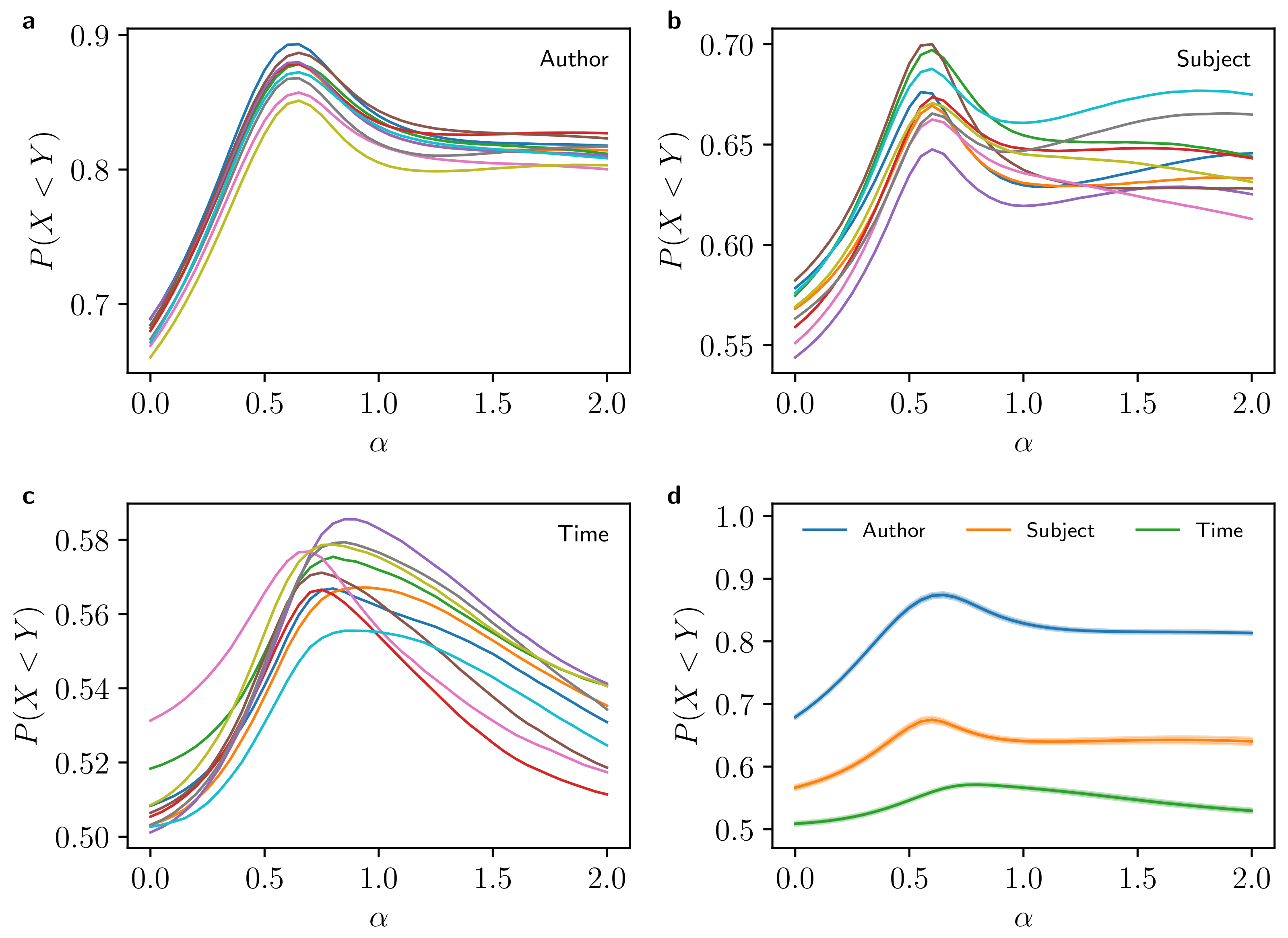
3.2. Jensen–Shannon Divergence

In Ref. [47], the bias of the estimator $D(\widehat{\mathit{p}},\widehat{\mathit{q}})$ is computed for texts of identical length. We extended this analysis by generalising it to allow for unequal sample sizes (specifically, when $N_{\widehat{\mathit{q}}}=N$ and $N_{\widehat{\mathit{p}}}=hN$, as stated previously).

As in Ref. [47], we see that the expression of the bias varies depending on whether $\alpha$ is larger or smaller than $1+1/\gamma$ (recall that $\gamma$ is the exponent of the Zipfian word-frequency distribution). In both cases, we found that the bias was a decreasing function of h when $h\in (1,h^{\ast })$, and increasing when $h>h^{\ast }$. This means that for a fixed N, there exists an optimal relation between text lengths, $h^{\ast }$, for which the bias is minimised. The bias formulations and corresponding $h^{\ast }$ values are displayed in

Table 2. Summary of analytical results for the Jensen–Shannon divergence, where $h^{\ast }$ denotes the critical value of h for which the bias of $D_{\alpha }$ is minimised. See Appendix D for a full derivation.

Range	$\mathit{Bias}\left[{\mathit{D}}_{\mathit{\alpha }}(\widehat{\mathit{p}},\widehat{\mathit{q}})\right]$	${\mathit{h}}^{\ast }$
$\alpha >1+1/\gamma$	$\frac{c\alpha }{2N}\left(\frac{1}{2h}+\frac{1}{2}-\frac{1}{h+1}\right)$	$1+\sqrt{2}$
$\alpha <1+1/\gamma$	$\frac{c\alpha }{2}\left(N^{-\alpha +1/\gamma }\right)\left(\frac{1}{2}{h}^{-\alpha +1/\gamma }+\frac{1}{2}-{(h+1)}^{-\alpha +1/\gamma }\right)$	$\frac{2^{\frac{\gamma }{1-\gamma -\alpha \gamma }}}{1-2^{\frac{\gamma }{1-\gamma -\alpha \gamma }}}$

, with a full derivation presented in Appendix D.

From the above formulations, we can also observe how the bias decays as the text length N grows. When $\alpha >1+1/\gamma$, the decay of the bias is $1/N$, and $\mathrm{Bias}\left[D_{\alpha }(\widehat{\mathit{p}},\widehat{\mathit{q}})\right]\to 0$ as $N\to \infty$. When $1/\gamma <\alpha <1+1/\gamma$, the bias again decays to zero, but does so sublinearly. Finally, when $\alpha <1/\gamma$, the bias diverges as $N\to \infty$, and thus, the estimator $D_{\alpha }(\widehat{\mathit{p}},\widehat{\mathit{q}})$ also diverges.

4. Numerical Results

We begin with a numerical performance comparison of our dissimilarity measures, before conducting an investigation into the effect of varying text lengths.

4.1. Numerical Performance Comparison

4.1.1. Vocabularies

We compared the Jaccard distance and overlap dissimilarity, and found that the Jaccard distance led to significantly higher $P(X<Y)$ values in all three tasks (p-value $<{10}^{-7}$, using two-sided paired t-tests). Based on these results, we chose to focus on the Jaccard distance in the subsequent analysis. These results are displayed in

Table A1. Performance of vocabulary dissimilarity measures. The quantity $P(X<Y)$ is displayed for each measure, and the given p-values are from paired t-tests and are two-sided.

Task	Jaccard	Overlap	p-Value
Author	0.796 ± 0.013	0.670 ± 0.007	$2.656\times {10}^{-9}$
Subject	0.633 ± 0.013	0.504 ± 0.012	$7.153\times {10}^{-8}$
Time period	0.595 ± 0.009	0.478 ± 0.007	$9.227\times {10}^{-10}$

.

4.1.2. Word Frequencies

Since the choice of parameter $\alpha$ in the generalised Jensen–Shannon divergence affects how different frequency ranges are weighted, we sought to identify which value optimised performance across our three tasks. Figure 1a–c show the performance of the generalised JSD across the parameter space $\alpha \in [0,2]$ for each of our three tasks. All three plots indicate a clear global maximum, at $\alpha ={\alpha }^{\ast }=0.65$ for the author task, ${\alpha }^{\ast }=0.6$ for subjects, and ${\alpha }^{\ast }=0.8$ for time periods. The curves also exhibit largely similar structure, with the main notable exception being the emergence of a second, local maximum in the region $\alpha \in [1.4,2]$ for some iterations of the subject task evaluation. Figure 1d compares the performance between tasks.

It is worth noting the difference in performance between the optimal $\alpha$ values, denoted by ${\alpha }^{\ast }$, and the value $\alpha =1$, which recovers the standard JSD in Equation (5).

Table A2. Performance comparison of the generalised JSD for $\alpha =1$ and $\alpha ={\alpha }^{\ast }$. The quantity $P(X<Y)$ is displayed for each measure, and the given p-values are from paired t-tests and are two-sided.

Task	JSD, $\mathit{\alpha }=1$	JSD, $\mathit{\alpha }={\mathit{\alpha }}^{\ast }$	p-Value
Author	0.8288 ± 0.0035	0.8743 ± 0.0038	$1.901\times {10}^{-10}$
Subject	0.6408 ± 0.0038	0.6749 ± 0.0048	$1.862\times {10}^{-5}$
Time period	0.5664 ± 0.0030	0.5712 ± 0.0026	$1.630\times {10}^{-2}$

provides the p-values for the paired t-tests between the $P(X<Y)$ calculations for the two $\alpha$ values. When using the Bonferroni adjusted threshold $0.05/3=1.6\times {10}^{-2}$, we see that all three results are significant, acknowledging that the significance for the time period task is marginal. These results indicate the value of considering entropies other than the popular and widely used Shannon entropy when using the Jensen–Shannon divergence, as it may potentially lead to improved performance depending on the application.

A surprising result in the above analysis is that the optimal performance occurred at very similar values of the parameter $\alpha$. We might have expected that different ranges on the frequency spectrum would have been emphasised for the different tasks. For example, the distribution of high-frequency words may have indicated stylometry and thus authorship variations, while low-frequency keywords may have been more useful for distinguishing between subjects. Our results, however, suggest that in general, penalising common words and emphasising low-frequency words improves our ability to distinguish between documents. This aligns with Ref. [24], where the authors found that subsampling common words led to practical benefits, including accelerated model learning and an improved accuracy of the learned vectors of rare words. Their heuristic subsampling strategy—Equation (5) in Ref. [24]—resulted in an effective reduction of the difference between the frequency of words, with words with frequency f appearing with frequency proportional to $\sqrt{f}$ after subsampling. This is effectively what is achieved using JSD with $\alpha <1$ (with $\alpha =0.5$ reproducing their square-root heuristic) and our finding of ${\alpha }^{\ast }<1$ can be seen as an information-theoretic justification for this proposed heuristic.

Another possible explanation for the position of ${\alpha }^{\ast }$ is the influence of the critical value of $\alpha$ discussed in Ref. [46]. There, it is shown that if word frequencies follow Zipf’s law, then for all $\alpha <{\alpha }_c=1/\gamma$, $H_{\alpha }$ and $D_{\alpha }$ diverge as the vocabulary size increases. When using the parameter estimates found in Ref. [48], we obtained ${\alpha }_c\approx 1/1.77\approx 0.56$, which was close to our optimal ${\alpha }^{\ast }$ values. Due to the finite number of words in our database, we could not increase the vocabulary size without bound, and thus we did not empirically observe $H_{\alpha },D_{\alpha }\to \infty$. However, there was still a finite-size effect that depended on the lengths of the texts being used, and this may have been influencing our results.

A third factor potentially causing the surprising similarity between our optimal $\alpha$ values is a confounding between the three different features—author, subject, and time period. To investigate this, we repeated our analysis on controlled subcorpora that sought to mitigate confounding. For the author task, each corpus was limited to one subject within a 50-year period. For distinguishing between subjects, we again limited to a 50-year period, and for the time period tasks, we restricted the corpora to one subject (see our repository [32] for further details about these filtered subcorpora). We found that controlling the subcorpora led to a much greater variability in the curves of $\alpha$ against $P(X<Y)$, with local maximums occurring at different points on the $\alpha$ spectrum. Importantly, however, we found that when we averaged over our 10 subcorpora, the peaks were very close to those we computed on the uncontrolled corpora. We found that for the author task, the maximum occurred at ${\alpha }^{\ast }=0.7$, while the strongest performance for both the subject and time period tasks was at ${\alpha }^{\ast }=0.6$.

4.1.3. Embeddings

Across all three tasks, the difference in performance between the Euclidean and Manhattan distances was not statistically significant, with p-value $>0.3$ for all three paired t-tests. The angular distance led to a stronger performance in the author and subject tasks, and this improvement was statistically significant (p-value $<{10}^{-5}$ for comparisons with both Manhattan and Euclidean distances). Conversely, the angular distance resulted in a significantly reduced performance in the time period task (p-value $<{10}^{-3}$ when comparing with either Manhattan or Euclidean distance). Thus, we conclude that the angular distance is the optimal distance measure for distinguishing between both authors and subjects. The Manhattan distance was optimal for the time period task, but its average performance increase over the Euclidean distance was marginal ($0.5357\pm 0.0034$ compared to $0.5354\pm 0.0034$). The full results can be found in

Table A3. Performance comparison of vector embedding approaches. The quantity $P(X<Y)$ is displayed for each measure, and the given p-values are from paired t-tests and are two-sided.

Task	Euclidean	Manhattan	Angular
Author	0.8448 ± 0.0026	0.8447 ± 0.0026	0.8599 ± 0.0025
Subject	0.6847 ± 0.0042	0.6846 ± 0.0043	0.6966 ± 0.004
Time period	0.5354 ± 0.0034	0.5357 ± 0.0034	0.5293 ± 0.0035

, and the p-values described above are available in

Table A4. Two-sided, paired t-tests comparing the performance of embedding distance measures.

Task	Metric Pair	p-Value
	Euclidean–Manhattan	$0.3185$
Author	Angular–Manhattan	$1.316\times {10}^{-8}$
	Angular–Euclidean	$2.002\times {10}^{-8}$
	Euclidean–Manhattan	$0.4101$
Subject	Angular–Manhattan	$4.065\times {10}^{-6}$
	Angular–Euclidean	$3.110\times {10}^{-6}$
	Euclidean–Manhattan	$0.3221$
Time period	Angular–Manhattan	$2.202\times {10}^{-4}$
	Angular–Euclidean	$3.972\times {10}^{-4}$

.

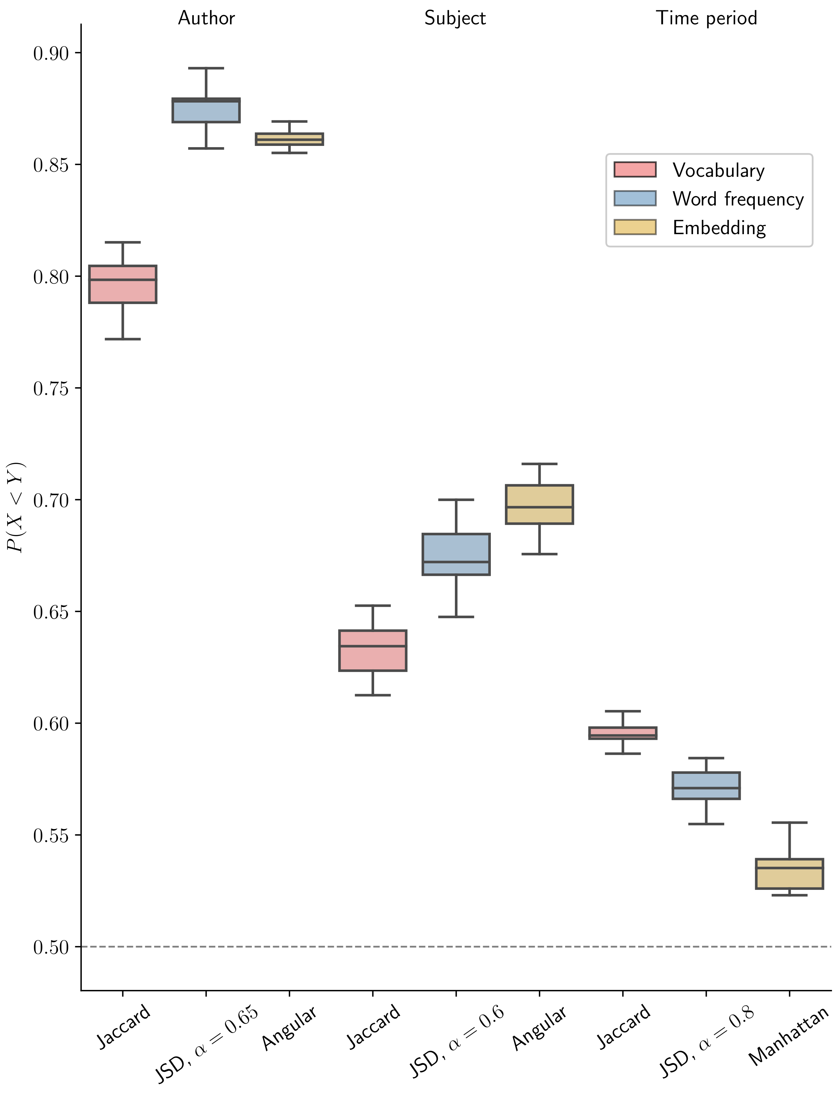
4.1.4. Overall Comparison

Figure 2 displays the performance of the optimal measures for each representation across our three tasks. Here, we see that the generalised Jensen–Shannon divergence with optimal parameter $\alpha =0.65$ had the strongest performance when distinguishing between texts written by different authors. Furthermore, the difference in performance between the optimal JSD and the second-strongest dissimilarity measure, the angular distance, was statistically significant ($p=2.951\times {10}^{-4}$). The Jaccard distance, which compares vocabularies, showed the weakest performance. It is perhaps surprising that a measure based on the simple bag-of-words model outperformed those based on vector embeddings. This suggests that the choices of words and their usage throughout a text are particularly useful for identifying stylistic differences between authors. It may also suggest that our vector embeddings were not fully capturing certain structural aspects of the texts that may be helpful for distinguishing between authors. Furthermore, we see that just comparing vocabularies is not sufficient; we also need to understand the distribution of those words throughout the text.

When evaluating the ability of our measures to distinguish between subjects, we see that the approaches based on vector embeddings were the strongest performers. This advantage over the second-strongest performer, the JSD with optimal parameter $\alpha =0.6$, was again statistically significant ($p=6.665\times {10}^{-4}$). As in the author task, we see that the measures based on vocabularies had the weakest performance. It is worth noting, however, that the average performance of the Jaccard distance ($0.6326\pm 0.0041$) was not far below that of the standard JSD ($0.6408\pm 0.0038$). The difference between them was still statistically significant ($p=1.306\times {10}^{-3}$), but this significance was marginal if we adjusted for multiple testing. Thus, we see that the embedding approach was the best approach for capturing textual differences between subjects. Clearly, a better representation of the semantic meaning of a text, rather than just the chosen words, leads to an improved ability to identify topical differences. Furthermore, vector embeddings are able to identify words and phrases that are synonymous, while the bag-of-words model cannot.

Rather surprisingly, the Jaccard distance had the strongest performance when distinguishing between time periods, despite its relative simplicity. Furthermore, the difference in performance between the Jaccard distance and the second-strongest measure, the JSD with $\alpha =0.8$, was highly significant, with a p-value of $5.374\times {10}^{-8}$. The measures based on vector embeddings performed relatively poorly and were only just above the baseline of 0.5. Languages change, develop, and grow over time, so it is reasonable to expect that the vocabulary of a text written today will differ from that of one written 200 years ago. What is surprising in these results, however, is that the JSD, which captures both vocabularies and word frequencies, underperformed the Jaccard distance. The poor performance of the embedding approaches suggests that while language may change over time, similar ideas and topics are being conveyed, and thus semantic meaning is not as useful for identifying temporal differences.

Additionally, Figure 2 visualises the inherent difficulty of each of our three tasks. Distinguishing between authors was the easiest of the three, with performance values typically ranging between 0.75 and 0.9. By comparison, it was very challenging for any of our dissimilarity measures to distinguish effectively between books written in different time periods. For this task, $P(X<Y)$ rarely exceeded 0.6, and was typically close to the baseline of 0.5. This underperformance is likely due to the overlap between the time periods caused by our estimation of the publication date. For the task of distinguishing between different subjects, we see that $P(X<Y)$ typically lay between 0.6 and 0.75.

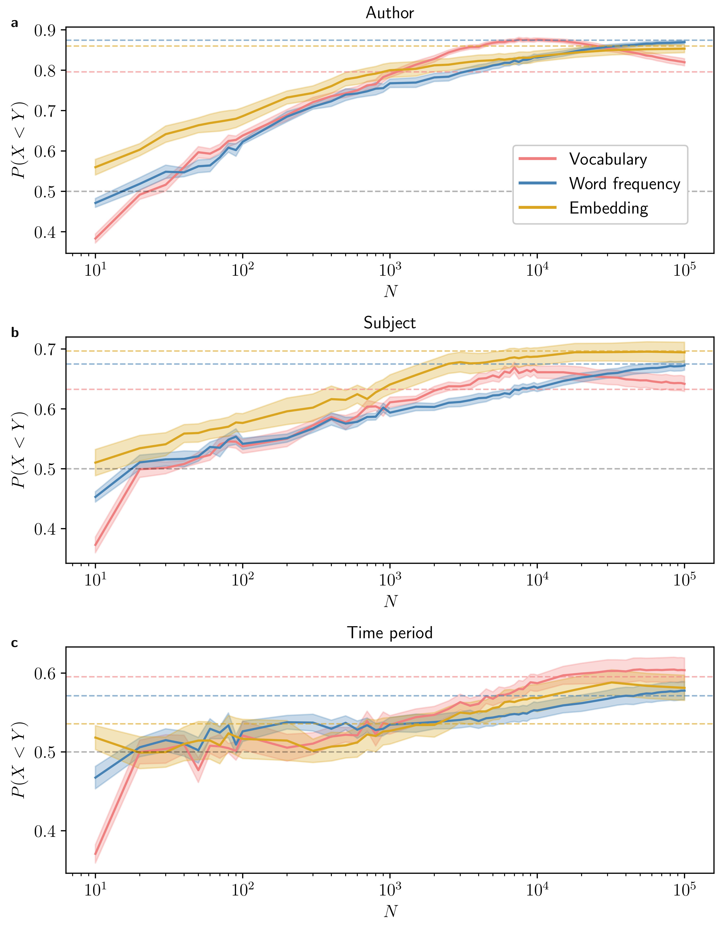
4.2. Dependence on Text Length

We first observed the impact of text length on performance, with the aim of determining the optimal measure for particular ranges of N. For each task, we selected the optimal dissimilarity measure for each of the three text representations—vocabularies, word frequencies and embeddings. For details of which measures were selected, refer to Section 4.1.

In Figure 3, we see that in both the author and subject tasks, the embedding approach led to a stronger performance for small text lengths, i.e., when $N\in [{10}^1,{10}^3]$. Thus, while our vocabulary or frequency measures may be appropriate for quantifying dissimilarity between large texts such as books, embedding approaches are more suitable for comparing short texts such as tweets or articles.

Interestingly, in both the author and subject tasks, the performance of the Jaccard distance appeared to peak at around $N={10}^4$. When generating a sample of size N, we generally expect to sample words that have frequency $1/N$ or greater. Thus, when resampling vocabularies, N is effectively a frequency cutoff—words with frequency greater than $1/N$ are likely to enter the vocabulary, while those with frequency less than $1/N$ likely will not. The peaks in our results seem to suggest that there exists an optimal $N^{\ast }$ such that if we only include words in our vocabulary with a frequency greater than $1/N^{\ast }$, our performance will be maximised.

The results on the time period task were less conclusive. We see that there was no clear optimal approach when comparing small texts. Importantly, the performance of all three approaches was very close to the baseline of 0.5. While this may indicate the innate difficultly of distinguishing between time periods when comparing small texts, it is likely also resulting from our approximation of publication date.

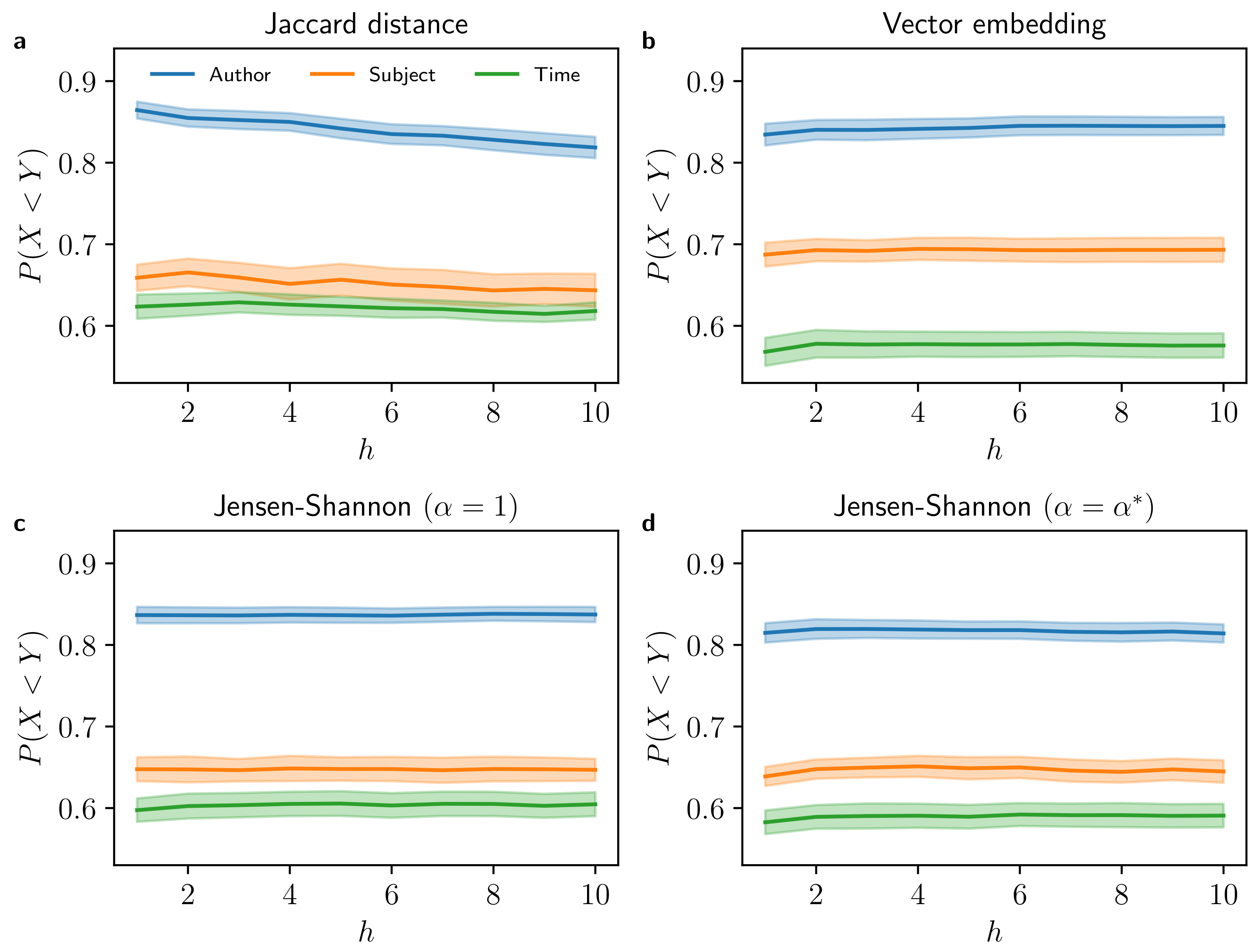
4.3. Impact of Unequal Text Length

From Figure 4, we see that the JSD and embedding-based approaches were robust against unbalanced text lengths, with performance remaining almost unchanged across all chosen h values (recall from Section 3 that $N_{\mathit{q}}=N$ and $N_{\mathit{p}}=hN$). The finding regarding the JSD may be connected to the bias computed analytically in Section 3.2—while the bias is dependent on h, it is negligible for large values of N, and thus the impact of unbalanced text length should be minimal. In contrast, the Jaccard distance was not robust, with all three representations showing a decreasing performance with increasing values of h. Again, this may be related to our analytical result in Section 3.1 regarding the lower bound of the Jaccard distance. Due to this bound, books that vary significantly in text length will receive high dissimilarity scores regardless of how fundamentally different they are, which in turn will influence the calculation of $P(X<Y)$. However, in both cases, further investigation is required to fully establish causality.

Now, a possible way to extend the Jensen–Shannon divergence to account for unequal text lengths is by giving different weightings to the two distributions being compared [33,47]. Specifically, we say

$$D_{\alpha }(\mathit{p},\mathit{q})=H_{\alpha }({\pi }_{\left(\mathit{p}\right)}\mathit{p}+{\pi }_{\left(\mathit{q}\right)}\mathit{q})-{\pi }_{\left(\mathit{p}\right)}{H}_{\alpha }\left(\mathit{p}\right)-{\pi }_{\left(\mathit{q}\right)}{H}_{\alpha }\left(\mathit{q}\right),$$

(11)

where ${\pi }_{\left(\mathit{p}\right)}=N_{\mathit{p}}/(N_{\mathit{p}}+N_{\mathit{q}})$ and ${\pi }_{\left(\mathit{q}\right)}=N_{\mathit{q}}/(N_{\mathit{p}}+N_{\mathit{q}})$ (recall that $N_{\mathit{p}}$ and $N_{\mathit{q}}$ denote the lengths of texts $\mathit{p}$ and $\mathit{q}$, respectively). We found, however, that the use of these weightings led to a decreased performance across all $\alpha \in [0,2]$ for all three tasks. This result is likely explained by the variability in text length in our PG data; if $N_{\mathit{p}}\gg N_{\mathit{q}}$, then ${\pi }_{\left(\mathit{p}\right)}\approx 1$ and ${\pi }_{\left(\mathit{q}\right)}\approx 0$, meaning that $D_{\alpha }(\mathit{p},\mathit{q})\approx 0$. Thus, when comparing a large text with a comparatively small text, the weighted JSD will approach zero regardless of how different the two word frequencies are.

5. Discussion

A number of key results emerged from our numerical performance comparison of the chosen dissimilarity measures. One such observation was the consistently strong performance of the Jensen–Shannon divergence (JSD) across the three tasks. Importantly, we saw an improvement in performance over the standard JSD when using the generalised divergence $D_{\alpha }$ based on the $\alpha$-entropy (see Equation (7)), with the best results in all three tasks obtained when $\alpha \in [0.6,0.8]$. As with the standard JSD (recovered when $\alpha =1$), $D_{\alpha }$ can be written as a sum over word types, thus providing a clear interpretation of the dissimilarity between texts. Other potentially important aspects of this family of dissimilarity measures are that they satisfy the triangular inequality for $\alpha \in [0,2]$ [39], and that the properties of their estimators can be computed explicitly for the simple bag-of-words process, as done previously in Ref. [47] and extended here for the case of texts with different lengths. Further studies, particularly into how the parameter $\alpha$ weights particular groups of words on the word frequency spectrum, are needed to fully understand the appropriateness of different parameter choices for particular tasks and to interpret our finding that $\alpha <1$ is typically preferred (higher weight to low-frequency words [36]).

Ultimately, the choice of dissimilarity measure depends on the task, the texts being compared, the statistical and mathematical properties of the measures and their estimators, and the extent to which it is important to have interpretable dissimilarity measures. For instance, while the Jaccard distance between vocabularies is arguably the measure with the simplest interpretation, we found analytically and empirically that the effectiveness of the Jaccard distance was hindered when the two texts varied significantly in length (while, in contrast, the generalised JSD and embedding-based distances were all robust). Focusing only on performance, the results we obtained indicate that the optimal dissimilarity measure is task-dependent, with all three approaches—vocabularies, word frequency distributions, and vector embeddings—exhibiting optimal performance on a particular task. In addition, the length of texts in the corpus must be considered; measures based on vector embeddings consistently outperformed other approaches on small texts, with a likely explanation for this being that small samples were not sufficiently representative of the underlying vocabularies or word frequency distributions. When deciding on the appropriateness of a particular measure for research or application, one should weigh up the performance increase of embedding approaches with the more limited interpretability and control of statistical properties when compared to vocabulary and word frequency techniques.

Further research in this area would involve extending our analysis to other dissimilarity measures, and exploring additional properties, both analytically and numerically, of such measures. Through this more holistic and standardised approach, researchers may gain a better understanding of why particular measures are suitable for certain tasks, as well as which measures are most applicable for new and emerging NLP areas. Our work may also help to inform decisions made by industry or other users who may not have the time or resources to conduct extensive comparisons.

References

1. Pham, H.; Luong, M.T.; Manning, C.D. Learning distributed representations for multilingual text sequences. In Proceedings of the 1st Workshop on Vector Space Modeling for Natural Language Processing, Denver, CO, USA, 5 June 2015; pp. 88–94. [Google Scholar]
2. Steyvers, M.; Griffiths, T. Probabilistic Topic Models. In Handbook of Latent Semantic Analysis; Landauer, T.K., McNamara, D.S., Dennis, S., Kintsch, W., Eds.; Psychology Press: New York, NY, USA, 2007; pp. 427–448. [Google Scholar]
3. Jiang, N.; de Marneffe, M.C. Do you know that Florence is packed with visitors? Evaluating state-of-the-art models of speaker commitment. In Proceedings of the 57th Annual Meeting of the Association for Computational Linguistics, Florence, Italy, 28 July–2 August 2019; pp. 4208–4213. [Google Scholar]
4. Wang, Q.; Li, B.; Xiao, T.; Zhu, J.; Li, C.; Wong, D.F.; Chao, L.S. Learning deep transformer models for machine translation. arXiv 2019, arXiv:1906.01787. [Google Scholar]
5. Taghva, K.; Veni, R. Effects of Similarity Metrics on Document Clustering. In Proceedings of the Seventh International Conference on Information Technology: New Generations, Las Vegas, NV, USA, 12–14 April 2010; pp. 222–226. [Google Scholar]
6. Zheng, L.; Jiang, Y. Combining dissimilarity measures for quantifying changes in research fields. Scientometrics 2022, 127, 3751–3765. [Google Scholar] [CrossRef]
7. Dias, L.; Gerlach, M.; Scharloth, J.; Altmann, E.G. Using text analysis to quantify the similarity and evolution of scientific disciplines. R. Soc. Open Sci. 2018, 5, 171545. [Google Scholar] [CrossRef]
8. Tommasel, A.; Godoy, D. Influence and performance of user similarity metrics in followee prediction. J. Inf. Sci. 2022, 48, 600–622. [Google Scholar] [CrossRef]
9. Singh, K.; Shakya, H.K.; Biswas, B. Clustering of people in social network based on textual similarity. Perspect. Sci. 2016, 8, 570–573. [Google Scholar] [CrossRef]
10. Tang, X.; Miao, Q.; Quan, Y.; Tang, J.; Deng, K. Predicting individual retweet behavior by user similarity: A multi-task learning approach. Know. Based Syst. 2015, 89, 681–688. [Google Scholar] [CrossRef]
11. Gomaa, W.H.; Fahmy, A.A. A Survey of Text Similarity Approaches. Int. J. Comput. Appl. 2013, 68, 13–18. [Google Scholar]
12. Wang, J.; Dong, Y. Measurement of Text Similarity: A Survey. Information 2020, 11, 421. [Google Scholar] [CrossRef]
13. Vijaymeena, M.K.; Kavitha, K. A Survey on Similarity Measures in Text Mining. Mach. Learn. Appl. 2016, 3, 19–28. [Google Scholar]
14. Prakoso, D.W.; Abdi, A.; Amrit, C. Short text similarity measurement methods: A review. Soft Comput. 2021, 25, 4699–4723. [Google Scholar] [CrossRef]
15. Magalhães, D.; Pozo, A.; Santana, R. An empirical comparison of distance/similarity measures for Natural Language Processing. In Proceedings of the National Meeting of Artificial and Computational Intelligence, Salvador, Brazil, 15–18 October 2019; pp. 717–728. [Google Scholar]
16. Boukhatem, N.M.; Buscaldi, D.; Liberti, L. Empirical Comparison of Semantic Similarity Measures for Technical Question Answering. In Proceedings of the European Conference on Advances in Databases and Information Systems, Turin, Italy, 5–8 September 2022; pp. 167–177. [Google Scholar]
17. Upadhyay, A.; Bhatnagar, A.; Bhavsar, N.; Singh, M.; Motlicek, P. An Empirical Comparison of Semantic Similarity Methods for Analyzing down-streaming Automatic Minuting task. In Proceedings of the Pacific Asia Conference on Language, Information and Computation, Virtual, 20–22 October 2022. [Google Scholar]
18. Al-Anazi, S.; AlMahmoud, H.; Al-Turaiki, I. Finding similar documents using different clustering techniques. In Proceedings of the Symposium on Data Mining Applications, Riyadh, Saudi Arabia, 30 March 2016; pp. 28–34. [Google Scholar]
19. Webb, A.R. Statistical Pattern Recognition, 2nd ed.; John Wiley & Sons, Inc.: Chichester, UK, 2003; p. 419. [Google Scholar]
20. Blei, D.M.; Ng, A.Y.; Jordan, M.I. Latent Dirichlet Allocation. J. Mach. Learn. Res. 2003, 3, 993–1022. [Google Scholar]
21. Salton, G.; Buckley, C. Term-weighting approaches in automatic text retrieval. Inf. Process. Manag. 1988, 24, 513–523. [Google Scholar] [CrossRef]
22. Herdan, G. Type-Token Mathematics: A Textbook of Mathematical Linguistics, 1st ed.; Mouton & Co.: The Hague, The Netherlands, 1960. [Google Scholar]
23. Bengio, Y.; Ducharme, R.; Vincent, P.; Jauvin, C. A neural probabilistic language model. J. Mach. Learn. Res. 2003, 3, 1137–1155. [Google Scholar]
24. Mikolov, T.; Chen, K.; Corrado, G.; Dean, J. Efficient Estimation of Word Representations in Vector Space. arXiv 2013, arXiv:1301.3781. [Google Scholar]
25. Pennington, J.; Socher, R.; Manning, C. GloVe: Global Vectors for Word Representation. In Proceedings of the Conference on Empirical Methods in Natural Language Processing, Doha, Qatar, 25–29 October 2014; pp. 1532–1543. [Google Scholar]
26. Le, Q.; Mikolov, T. Distributed Representations of Sentences and Documents. In Proceedings of the 31st International Conference on Machine Learning, Beijing, China, 21–26 June 2014; pp. 1188–1196. [Google Scholar]
27. Hill, F.; Cho, K.; Horhonen, A. Learning Distributed Representations of Sentences from Unlabelled Data. In Proceedings of the Conference of the North American Chapter of the Association for Computational Linguistics: Human Language Technologies, San Diego, CA, USA, 12–17 June 2016; pp. 1367–1377. [Google Scholar]
28. Wu, L.; Yen, I.E.; Xu, K.; Xu, F.; Balakrishnan, A.; Chen, P.Y.; Ravikumar, P.; Witbrock, M.J. Word Mover’s Embedding: From Word2Vec to Document Embedding. In Proceedings of the Conference on Empirical Methods in Natural Language Processing, Brussels, Belgium, 31 October–4 November 2018; pp. 4524–4534. [Google Scholar]
29. Vaswani, A.; Shazeer, N.; Parmar, N.; Uszkoreit, J.; Jones, L.; Gomez, A.N.; Kaiser, L.; Polosukhin, I. Attention is All you Need. In Proceedings of the 31st Conference on Neural Information Processing Systems, Long Beach, CA, USA, 4–9 December 2017; pp. 6000–6010. [Google Scholar]
30. Devlin, J.; Chang, M.-W.; Lee, K.; Toutanova, K. BERT: Pre-training of Deep Bidirectional Transformers for Language Understanding. In Proceedings of the Conference of the North American Chapter of the Association for Computational Linguistics: Human Language Technologies, Volume 1 (Long and Short Papers), Minneapolis, MN, USA, 2–7 June 2019; pp. 4171–4186. [Google Scholar]
31. Radford, A.; Narasimhan, K.; Salimans, T.; Sutskever, I. Improving Language Understanding by Generative Pre-Training; Technical Report; OpenAI: San Francisco, CA, USA, 2018. [Google Scholar]
32. Shade, B. Repository with the Code Used in This Paper; Static Version in Zenodo; Dynamic Version in Github; 2023. Available online: https://doi.org/10.5281/zenodo.7861675; https://github.com/benjaminshade/quantifying-dissimilarity (accessed on 14 February 2022).
33. Lin, J. Divergence measures based on the Shannon entropy. IEEE Trans. Inf. Theory 1991, 37, 145–151. [Google Scholar] [CrossRef]
34. Cover, T.M.; Thomas, J.A. Elements of Information Theory, 1st ed.; John Wiley & Sons, Inc.: Hoboken, NJ, USA, 2005. [Google Scholar]
35. Endres, D.M.; Schindelin, J.E. A new metric for probability distributions. IEEE Trans. Inf. Theory 2003, 49, 1858–1860. [Google Scholar] [CrossRef]
36. Gerlach, M.; Font-Clos, F.; Altmann, E.G. Similarity of Symbol Frequency Distributions with Heavy Tails. Phys. Rev. X 2016, 6, 021109. [Google Scholar] [CrossRef]
37. Havrda, J.; Charvát, F. Quantification Method of Classification Processes. Concept of Structural α-Entropy. Kybernetika 1967, 3, 30–35. [Google Scholar]
38. Burbea, J.; Rao, C. On the convexity of some divergence measures based on entropy functions. IEEE Trans. Inf. Theory 1982, 28, 489–495. [Google Scholar] [CrossRef]
39. Briët, J.; Harremoës, P. Properties of classical and quantum Jensen-Shannon divergence. Phys. Rev. A 2009, 79, 052311. [Google Scholar] [CrossRef]
40. Reimers, N.; Gurevych, I. Sentence-BERT: Sentence Embeddings using Siamese BERT-Networks. In Proceedings of the 2019 Conference on Empirical Methods in Natural Language Processing and the 9th International Joint Conference on Natural Language Processing, Hong Kong, China, 3–7 November 2019; pp. 3982–3992. [Google Scholar]
41. Wang, W.; Wei, F.; Dong, L.; Bao, H.; Yang, N.; Zhou, M. MiniLM: Deep Self-Attention Distillation for Task-Agnostic Compression of Pre-Trained Transformers. In Proceedings of the 34th Conference on Neural Information Processing Systems, Virtual, 6–12 December 2020; pp. 5776–5788. [Google Scholar]
42. Beltagy, I.; Peters, M.E.; Cohan, A. Longformer: The Long-Document Transformer. arXiv 2020, arXiv:2004.05150. [Google Scholar]
43. Project Gutenberg. Available online: https://www.gutenberg.org (accessed on 8 February 2022).
44. Gerlach, M.; Font-Clos, F. A Standardized Project Gutenberg Corpus for Statistical Analysis of Natural Language and Quantitative Linguistics. Entropy 2020, 22, 126. [Google Scholar] [CrossRef]
45. Gerlach, M.; Font-Clos, F. Standardized Project Gutenberg Corpus, Github Repository. 2018. Available online: https://github.com/pgcorpus/gutenberg (accessed on 14 February 2022).
46. Altmann, E.G.; Dias, L.; Gerlach, M. Generalized entropies and the similarity of texts. J. Stat. Mech. Theory Exp. 2017, 2017, 014002. [Google Scholar] [CrossRef]
47. Gerlach, M. Universality and Variability in the Statistics of Data with Fat-Tailed Distributions: The Case of Word Frequencies in Natural Languages. Ph.D. Thesis, Max Planck Institute for the Physics of Complex Systems, Dresden, Germany, 2015. [Google Scholar]
48. Gerlach, M.; Altmann, E.G. Stochastic Model for the Vocabulary Growth in Natural Languages. Phys. Rev. X 2013, 3, 021006. [Google Scholar] [CrossRef]
49. Bird, S.; Klein, E.; Loper, E. Natural Language Processing with Python: Analyzing Text with the Natural Language Toolkit, 1st ed.; O’Reilly Media, Inc.: Sebastopol, CA, USA, 2009. [Google Scholar]
50. Egloff, M.; Adamou, A.; Picca, D. Enabling Ontology-Based Data Access to Project Gutenberg. In Proceedings of the Third Workshop on Humanities in the Semantic Web, Heraklion, Crete, Greece, 2 June 2020; pp. 21–32. [Google Scholar]
51. Mann, H.B.; Whitney, D.R. On a Test of Whether one of Two Random Variables is Stochastically Larger than the Other. Ann. Math. Stat. 1947, 18, 50–60. [Google Scholar] [CrossRef]
52. Mason, S.J.; Graham, N.E. Areas beneath the relative operating characteristics (ROC) and relative operating levels (ROL) curves: Statistical significance and interpretation. Q. J. R. Meteorol. Soc. 2002, 128, 2145–2166. [Google Scholar] [CrossRef]
53. Hanley, J.A.; McNeil, B.J. The meaning and use of the area under a receiver operating characteristic (ROC) curve. Radiology 1982, 143, 29–36. [Google Scholar] [CrossRef]
Figure 1. Performance P ( X < Y ) (Equation (8)) of the Jensen–Shannon divergence for different values of the parameter α (as defined in Equation (7)). (ac) Results for author, subject, and time period tasks, respectively. Each line shows the performance obtained on a unique subcorpus, see Section 2.2 for details. (d) Performance comparison between tasks, with the lines indicating average performance across the 10 subcorpora and shaded regions indicating standard error.
Information 14 00271 g001
Figure 2. Performance P ( X < Y ) (Equation (8)) of strongest measures for each text representation across the three tasks. The optimal measures for each text representation (vocabulary, word frequency, and embedding) and task (author, subject, time) are identified in Section 4.1.4. The boxplots show the distribution of P ( X < Y ) values for the 10 subcorpora.
Information 14 00271 g002
Figure 3. Performance P ( X < Y ) (Equation (8)) of our optimal measures as a function of text length N. (a) Author task; (b) subject task; (c) time period task. The optimal measures for each representation and task are identified in Section 4.1.4 and displayed in Figure 2. The solid lines indicate average performance across the 10 subcorpora, and the shaded regions indicate standard error. The dashed lines indicate the average performance of these measures computed using the original texts (see Section 4.1), and the grey line indicates the performance baseline of 0.5. In each iteration, texts were resampled to a fixed length N before computing P ( X < Y ) .
Information 14 00271 g003
Figure 4. Impact of h parameter (proportional difference in text length) on performance P ( X < Y ) (Equation 8)) of dissimilarity measures. (a) Jaccard distance; (b) optimal embedding measure for each representation; (c) standard JSD based on Shannon entropy; (d) generalised JSD with α = α . For each dissimilarity calculation, one text is resampled to length N, and the other to length h N , where N = 10,000 is fixed. The solid lines indicate average performance across the 10 subcorpora, and the shaded regions indicate standard error.
Information 14 00271 g004