Distilling Knowledge with a Teacher’s Multitask Model for Biomedical Named Entity Recognition ^†

Abstract

Single-task models (STMs) struggle to learn sophisticated representations from a finite set of annotated data. Multitask learning approaches overcome these constraints by simultaneously training various associated tasks, thereby learning generic representations among various tasks by sharing some layers of the neural network architecture. Because of this, multitask models (MTMs) have better generalization properties than those of single-task learning. Multitask model generalizations can be used to improve the results of other models. STMs can learn more sophisticated representations in the training phase by utilizing the extracted knowledge of an MTM through the knowledge distillation technique where one model supervises another model during training by using its learned generalizations. This paper proposes a knowledge distillation technique in which different MTMs are used as the teacher model to supervise different student models. Knowledge distillation is applied with different representations of the teacher model. We also investigated the effect of the conditional random field (CRF) and softmax function for the token-level knowledge distillation approach, and found that the softmax function leveraged the performance of the student model compared to CRF. The result analysis was also extended with statistical analysis by using the Friedman test.

1. Introduction

Vast amounts of valuable information are being shared online through textual data that are posted at an extremely high rate. However, much of these data are unstructured, rendering the manual processing of such large amounts of unstructured text data challenging and tedious. Processing such large amounts of unstructured data needs intelligent domain-based techniques.

Natural language processing (NLP), a branch of artificial intelligence, processes unstructured textual data [1] on the basis of user demand. NLP allows for computer systems to understand, interpret, and manipulate human language, and it has been implemented for many tasks, such as sentiment analysis, information extraction, and topic searching and modeling. Information mining (IE) is a technique for extracting related data from unstructured text [2] that has been extended to several subtasks, of which one is entity recognition (NER). A named entity is a proper noun that appears in a sentence. NER recognizes the text of interest and maps it to predefined categories such as people, geographic locations, and organizations. NER can be viewed as a sequence tagging problem determining the output tags of input words presented in sentences [3].

As the number of published biomedical texts has increased, IE has also become an essential activity in the biomedical field. Biomedical named entity recognition (BioNER) recognizes and associates biomedical facts to predefined categories such as genes, chemicals, and diseases [4]. BioNER tasks are more difficult to implement than usual NER tasks because the biomedical literature differs in many ways from standard text data. Although there are certain conventions observed by researchers to describe biomedical concepts, there are still no hard and fast rules governing the biomedical field. It is becoming increasingly difficult to follow the same naming conventions in the open and growing biomedical literature. Another issue concerns entity classification. Different human annotators, even from the same background, may associate the same words with different medical concepts, e.g., “p53" corresponds to a protein in the GENIA corpus. In contrast, the HUGA nomenclature annotates it as a gene: “TP53”.

The use of different spellings for the same entity is also very common in biomedical texts. For example, IL12, IL 12, and IL-12 refer to the same entity, but use different spelling conventions [5]. Another challenge for BioNER is learning synonyms that appear in the text. For example, PTEN and MMAC1 represent the same genetic entity, but have different synonyms.

Moreover, long compound word entities complicate the training process of the BioNER model because these entities are represented by character types. For instance, “10-ethyl-5-methyl-5,10-dideazaaminopterin” and “12-o-tetradecanoylphorbol 13-acetate” contain alphanumerical and special characters. Different tokenizers treat these special characters differently. Therefore, applying different tokenizers may result in different outputs for the same entity. Descriptive entities such as “pigment-epithelium-derived factor” and “medullary thymic epithelial cells” hinder entity boundary identification. Biomedical entities may also comprise nested entities; e.g., “CIITA mRNA” symbolizes a reference to RNA, but “CIIT” refers to DNA [6].

Furthermore, a common practice in writing biomedical texts is to use entity acronyms that may refer to different entities. For instance, “TCF” can refer to “tissue culture fluid” or “T-cell factor” [7]. Similarly, “EGFR” can stand for “estimated glomerular filtration rate” or “epidermal growth factor receptor”. Determining acronyms for a particular entity is associated with the context of the sentence. Distinguishing such entities from each other is another challenging aspect for BioNER systems.

Due to the aforementioned limitations, BioNER tasks are more difficult than common NER tasks. Although early BioNER systems are effective, their overall performance continues to be restricted by the open and expanding biomedical literature. Traditional machine-learning algorithms show improved results compared to early dictionary-based and rule-based methods. However, machine-learning algorithms require a manual feature-engineering step that directly affects the performance of the model. Distinctive features could improve performance, while redundant and irrelevant features worsen performance.

More advanced methods rely on deep-learning techniques, eliminating the need for manual feature engineering while still providing the required outcome. A deep-learning (DL) architecture consists of several layers that help in exploring the properties and complex structure of data layer by data layer. The latent ability of DL models to learn complex features was successfully demonstrated in various domains, e.g., speech recognition [8], drug discovery [9,10], the clinical setting [11], and computer vision [12].

Even though deep-learning models produced state-of-the-art results in many fields, the structure of these models is very complex and requires extensive computational power for training. Sutskever et al. [13] proposed a model that comprised 4 layers of LSTMs that each had 1000 hidden units. Similarly, the model presented by Zhou et al. [14] had multilevel LSTMs, and each layer comprised 512 hidden units. With millions of parameters, these models are computationally expensive to train. These cumbersome models also require more storage space, rendering them unsuitable for deployment with real-time data. One example is to use them on a cellphone, where limited storage and computational power are available. As a result, it is necessary to compress these complex models while preserving the generalization that they have learned—-in other words, without jeopardizing the performance of these deep-learning models. In this case, the knowledge distillation approach is utilized to compress a cumbersome model into a simple model, allowing for implementing it in end-user devices with less computational power [15]. This work proposes the distillation knowledge approach to leverage the performance of deep-learning models. Instead of compressing the model, this research aims to maximize the efficiency and performance of the models.

Our previous work [16] used a multitask learning (MTL) approach to leverage the performance of BioNER. The performance of the multitask model (MTM) is usually restricted or improved due to loss optimization via the joint training of different tasks. Data distribution from different tasks renders the MTM overfitted for some tasks and underfitted for other tasks. The knowledge distillation approach can overcome such limitations through, for example, the student model learning not only from the available inputs, but also through the output of the teacher model. Consequently, this article presents different knowledge distillation approaches to boost the performance of deep neural network models.

2. Knowledge Distillation

In knowledge distillation, the goal is to train one model with the representations learned from another model. The aim of distilling knowledge could be achieved by training a simple model (student) on the knowledge gained through a complex model (teacher). In particular, the knowledge distillation approach concerns how the generalizations of one, often complex (teacher), model can be transferred to another model, usually a simple (student) model. Complex models or ensemble approaches are more effective than simple single-task models are, but require more computational power to train. Knowledge distillation enables simple (student) models to perform better than single or ensemble models. In this way, the student model can be trained with fewer training examples because, during training, it also uses the knowledge gained from the teacher model. The idea is that, during training, a complex model is generalized to the data. This helps the student’s model in matching the teacher’s model or in approaching generalization. A learning model learns not only via its implicit knowledge, but also through the gradients of other knowledge.

The transmission of knowledge from the teacher model is often achieved through the output probabilities of the teacher model. The goal of any learning model is obviously the prediction of the right label for the input instance. The model, therefore, assigns a high probability to that specific class, while the remaining classes are represented with small probability values. The association of probabilities with the rest of the false labels is not arbitrary. These side probabilities also contain representations describing how a particular model generalizes the classes. For example, it is quite unlikely that the image of a car would be misclassified as the image of a motorcycle, but highly likely to be misclassified as an image of a truck. The softmax activation function produces a probability distribution for each class for a specific instance. These generated probability distributions sum to 1. These softmax probabilities carry additional hidden information than that of one-hot “hard labels”. For instance, softmax probability [0.7, 0.2, 0.1] indicates the ranks of the class. Such information cannot be identified with rigid labels, e.g., [1, 0, 0]. These posterior probabilities can provide additional effective signals to the student model during training. However, training a student model that fits these probabilities may not be very effective, as the student model may only consider the highest probability values. One way to reduce the impact of high probability values is the normalization of these final output probabilities [17]. Normalized probabilities represent soft labels with more knowledge available to the student model [18]. The student model then looks at other values in addition to the most probable class. Hinton et al. [17] proposed a tuneable parameter term temperature, $\tau$, to soften the posterior probabilities, as given in Equation (1).

$$\mathrm{Softmax}\left(z_i\right)=\frac{exp(z_i/\tau )}{{\sum }_{j}exp(z_j/\tau )}$$

(1)

Introducing this new $\tau$ parameter normalizes the output probabilities; e.g., setting the value of $\tau =3$ for the above softmax output yields [0.375, 0.317, 0.307]. The output probabilities are softened, but the potential class rankings do not change. In addition, the student model then looks for other nonclass values. A high value of $\tau$ normalizes the softmax output, rendering nontarget class output probability prominent [19]. Keeping $\tau =1$ renders it a standard softmax function. A large value of $\tau$ softens the softmax output and enhances the nontarget class output probability [19], and the probability value of the target class also decreases to some extent. Therefore, it is important to choose an appropriate value for the temperature parameter.

3. Proposed Knowledge Distillation Approach

The proposed knowledge distillation approach [20] is shown in Figure 1. The teacher model is an MTM that uses sentence, word, and character input representations. The top layer of MTMs, indicated by black rounded rectangles, was shared by all datasets. The lower layer, represented by a red rounded rectangle, was dataset-specific, and the softmax function was used to label the output. Jointly training on the associated tasks allows for an MTM to learn common features among different tasks by using shared layers [21]. The joint training of related tasks also enables the model to optimize its parameters for different tasks, thus reducing the possibility of overfitting for a particular task. Task-specific layers learn features that are more relevant to the current task.

Such a behavior of MTM can also be transferred to the student model with the help of the knowledge distillation approach. Thus, an MTM (right-hand side of Figure 1) is a teacher model used in the experiments presented later in this paper. Furthermore, this research aims to achieve knowledge distillation at the token level. For this reason, the proposed approach uses a softmax function that generates token-level probability distribution. Conditional random fields (CRFs) predict labels for entire sequences, so token-level knowledge extraction is not possible. CRF-based models label sequences by considering associations between adjacent labels. This confines knowledge extraction from the teacher model [22]. To test this hypothesis, we implemented a teacher MTM with a CRF at the output layer (Section 5.4).

The student model was in fact a counterpart STM of the MTM. As such, the STM was a student model that had been trained without a knowledge distillation approach. Therefore, the structure of the two models was the same. The proposed approach utilizes different layers of MTM for knowledge distillation. The deep-learning model comprehends complex features from the generic to the abstract levels, layer by layer. Different intermediate layers of the teacher model are used for knowledge distillation. This includes a shared BiLSTM layer, a task-specific BiLSTM layer, and hidden layer logits (refer Figure 1). As such, the student model was trained in a guided way at different levels; therefore, this may improve the performance of the student model. Layer knowledge was integrated from the logit layer to different layers step by step in different experiments to observe the effects of each integration. The logits (input to the softmax layer [23]) carry values in the range of $[-\infty ,+\infty ]$, corresponding to unmasked information; therefore, feature representation at this level is more beneficial and refined. The softmax function uses logits to produce the probability distribution of class labels, which causes the loss of hidden knowledge present in the logit layer. Considering that, this paper also contains experiments in which a student model was trained on the logits of the MTM. However, to validate this hypothesis, knowledge distillation is also performed at the softmax layer using soft labels where the output probability distribution of the teacher model is softened by tuneable parameter $\tau$.

This work also explores the advantages of ensemble methods in two different ways. First, the logits (input to the softmax layer [23]) of different MTMs were combined to train the student model. The MTMs used in the ensemble method had the same architecture, but were initialized with different seed values, resulting in MTMs with different trained weights. The combined logits were averaged and then used to distill knowledge to the student model. The second method, the ensemble approach, averages the logits of CRF-based and softmax-based MTMs to train the student model (SM). The rationale for this approach is that different MTMs learn different feature sets, so the SM is trained with a wider range of features.

During training, the SM considers the actual labels and distillation loss that depend on the results by matching the outputs of the teacher model (MTM). For the intermediate layers’ knowledge distillation loss, mean-squared error (MSE) is calculated to minimize the loss between student and teacher predictions at the different layers. When soft labels are considered, on the other hand, cross-entropy loss is used.

4. Experimental Settings

The MTM shown on the right-hand side of Figure 1 was trained separately with an MTL approach using all the datasets presented in this paper and was then utilized for knowledge transformation into the student model (SM) [24]. When the knowledge distillation was performed using the logits of the hidden layer, Equation (2) was used to compute the loss of the SM. The knowledge distillation loss was the MSE of the teacher and the student logits. Here, x represents the input, W represents SM parameters, $\mathcal{H}$ is the cross-entropy loss, y corresponds to the true labels, and $\sigma$ is the softmax function applied to the teacher logits, $z_s$, and student logits, $z_t$. $\alpha$ and $\beta$ are hyperparameters to quantify each loss.

The experiments were conducted to consider different $\alpha$ values, i.e., $[0,0.5,1]$ whereas $\beta =1-\alpha$. Hyperparameter tuning for $\alpha$ and $\beta$ was not performed, and the values were naively chosen. If $\alpha =0$, the SM learnt with only distillation loss, while choosing $\alpha =0.5$ equally used both student loss and distillation loss. Lastly, $\alpha =1$ enabled the SM to utilize student loss. $\alpha =1$ transformed the SM into a single-task model (STM). The SM, however, still utilized the logits of the teacher model during its training phase. This helps the SM in learning and modifying the weights of layers during the backpropagation phase.

When knowledge distillation is carried out at the task-specific BiLSTM layer along with the logits of the hidden layer, the loss is computed using Equation (3). The new parameter, $\gamma =[0,0.5,1]$, weighs the matching loss at the task-specific BiLSTM layer. The hyperparameters are tuned to select the best value for $\alpha ,\beta , \mathrm{and} \gamma$. When the knowledge of the shared BiLSTM was incorporated with the above layer’s knowledge, the loss was calculated using Equation (4). The MSE error of the task-specific BiLSTM was controlled using the new parameter, $\kappa =[0,0.5,1]$. For Equation (4), hyperparameter tuning was performed for $\beta ,\gamma , \mathrm{and} \kappa$ to select the best value from $[0,0.5,1]$ for each parameter, while $\alpha$ was kept constant at 1. When knowledge distillation was carried out using soft labels, Equation (5) was used to calculate the loss. Parameters $\alpha$ and $\beta$ were retained at 0.5, while $\tau$ was finetuned for each dataset. All our results were over the course of five runs, and each run was executed with different seed values. The reported F1 scores are, therefore, based on five runs.

$$\mathcal{L}(x;W)=\alpha ·\mathcal{H}(y,\sigma (z_s,z_t))+\beta ·MS{E}_{logits}$$

(2)

$$\mathcal{L}(x;W)=\alpha ·\mathcal{H}(y,\sigma (z_s,z_t))+\beta ·MS{E}_{logits}+\gamma ·MS{E}_{TaskSpecific}$$

(3)

$$\mathcal{L}(x;W)=\alpha ·\mathcal{H}(y,\sigma (z_s,z_t))+\beta ·MS{E}_{logits}+\gamma ·MS{E}_{TaskSpecific}+\kappa ·MS{E}_{Shared}$$

(4)

$$\mathcal{L}(x;W)=\alpha ·\mathcal{H}(y,\sigma (z_s,z_t))+\beta ·\mathcal{H}(y,\sigma (z_s/\tau ,z_t/\tau ))$$

(5)

Our experiments considered 15 datasets [25] that had also been used by Wang et al. [26], and Crichton et al. [27]. The biological entities in these datasets are diseases, species, cellular components, cells, genes, proteins, and chemicals. Each dataset contains a training set, a validation set, and a test set. We followed a similar experimental setup to that of Wang et al. (https://github.com/yuzhimanhua/Multi-BioNER, accessed on 10 February 2023), where the model was trained using both the training set and validation set.

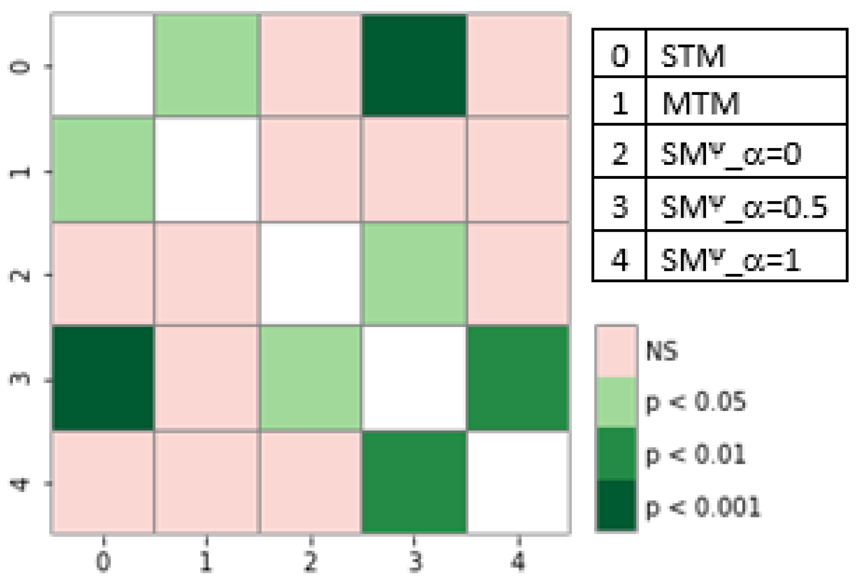
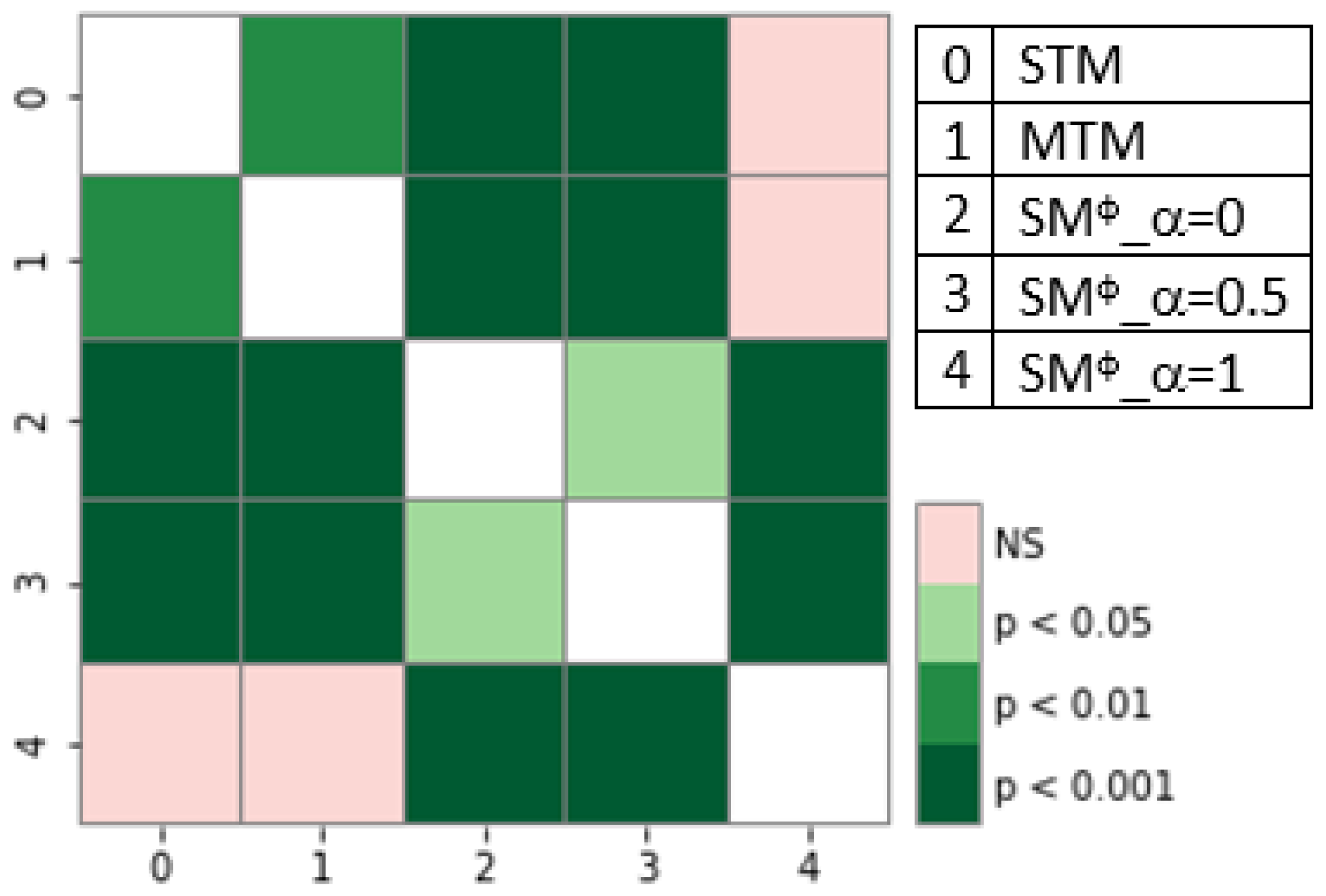
We also performed detailed statistical analysis, and used graphs to find statistical significance between the different results so that they could be better represented. Statistical analysis was performed using the Friedman test [28] to determine the statistical significance of the differences in the results of the different models.

5. Results and Discussions

5.1. Knowledge Distillation Using Logits of the Teacher Model

Table 1. Result comparison of the $S{M}^{\psi }$ trained with logits of the softmax-based teacher MTM.

Datasets	STM	MTM	${\mathit{SMs}}^{\mathit{\Psi }}$
			$\mathbf{\alpha }=\mathbf{0}$	$\mathbf{\alpha }=\mathbf{0}.\mathbf{5}$	$\mathbf{\alpha }=\mathbf{1}$
AnatEM	86.7	86.7	87.1	87.1	87.3
BC2GM	81.2	80.0	80.7	81.1	81.4
BC4CHEMD	90.1	86.6	89.3	89.4	89.4
BC5CDR	88.0	87.3	87.4	87.9	88.1
BioNLP09	87.6	88.3	88.8	88.4	88.7
BioNLP11EPI	82.7	84.4	84.2	84.7	82.9
BioNLP11ID	85.7	87.2	87.0	87.1	85.9
BioNLP13CG	82.1	84.0	82.9	83.6	82.5
BioNLP13GE	75.6	79.3	77.6	77.8	75.4
BioNLP13PC	86.8	88.6	88.0	88.3	87.2
CRAFT	84.4	82.3	82.6	84.0	84.5
ExPTM	73.5	80.9	76.1	76.5	73.6
JNLPBA	70.8	70.3	70.6	72.1	71.2
linnaeus	87.4	88.4	88.5	88.4	87.5
NCBI	84.3	85.0	84.9	85.3	84.2
Average	83.1	83.9	83.7	84.1	83.3

presents the result comparison of the $SM{s}^{\psi }$ with STM and MTM (a teacher model). $SM{s}^{\psi }$ outperformed most of the datasets compared with the STM except for BC4CHEMD. MTM results for BC4CHEMD show that the MTM was not able to improve the results for these datasets. This might be the reason why $SM{s}^{\psi }$ were not able to learn sufficient knowledge from the MTM. However, $SM{s}^{\psi }$ improved the results for BC4CHEMD compared with the MTM, showing the benefits of the knowledge distillation approach. The $S{M}^{\psi }(\alpha =0.5)$ trained with both student loss and distillation loss was more effective, yielding an average F1 score of 84.1. The $S{M}^{\psi }(\alpha =0)$ trained with only knowledge distillation loss had the second-best score, with an average F1 score of 83.7.

Statistical Analysis of $S{M}^{\psi }$

Statistical analysis was also performed on the results of Table 1 using the Friedman test to find out if the differences in the results from different models were statistically significant. Figure 2 represents the results of the output of the statistical analysis. Only one knowledge distillation model, $S{M}^{\psi }(\alpha =0.5)$, produced statistically significant results regarding STM. However, when the results were compared with those of the MTM (teacher model), no distillation model $S{M}^{\psi }$ was able to deliver statistically significant results. $S{M}^{\psi }(\alpha =0.5)$ produced statistically significant results against other variants, i.e., $S{M}^{\psi }(\alpha =0)$ and $S{M}^{\psi }(\alpha =1)$.

Figure 3 depicts the graphical representation of the model on the basis of the generated ranks with the Friedman test. For better understanding, different colors are used for the rectangles and arrows, where the arrow has the same color as that of the rectangle to which it belongs. $S{M}^{\psi }(\alpha =0.5)$ produced the best results among all the models. Other knowledge distillation models ($S{M}^{\psi }(\alpha =0)$ and $S{M}^{\psi }(\alpha =1)$) also resulted in fewer ranks than those of the teacher model (MTM). The results of $S{M}^{\psi } \mathrm{with} (\alpha =1)$ were the worst among the $SM{s}^{\psi }$.

5.2. Knowledge Distillation Using an Ensemble Approach

In machine learning, ensemble approaches are more effective than a single machine-learning model approach. Deep-learning models are nonlinear and thereby produce a different set of weights when a single model is trained each time. The initial weights can also cause different predictions, resulting in high variance in the predictions. To reduce that variance, various neural network models can be trained and combined to generate a single prediction. Furthermore, a single model might not necessarily learn distinctive features in the data. This limitation can be tackled in the ensemble approach, where feature representations from different models are combined into a single ensemble model. The predictions from different models can be combined using different methods, including voting, average, and weighted voting/average schemes.

This section introduces two types of ensemble methods where different predictions are combined using a weighted average scheme. In this scheme, predictions from different models are averaged and combined according to their estimated performance. In this section, feature representation at the logit layer is combined from various models, which enhances the learning ability of the SM to learn from a wide range of feature representations. The architecture of the teacher MTMs used in the experiments was the same, but their weights were initialized randomly with different seed values, ensuing different predictions. In the first proposed approach, $SM{s}^{\varphi }$ used logits from an ensemble of MTMs to train the $S{M}^{\varphi }$. The averaged logits of these MTMs were used to train the $S{M}^{\varphi }$. In the second ensemble approach, the averaged logits of softmax-based MTMs and CRF-based MTMs were used to train the $S{M}^{\mathrm{\S }}$.

Table 2. Result comparison of $S{M}^{\varphi }$ trained with the logits of the ensemble teacher softmax-based MTMs.

Datasets	STM	MTM	${\mathit{SMs}}^{\mathit{\varphi }}$
			$\mathbf{\alpha }=\mathbf{0}$	$\mathbf{\alpha }=\mathbf{0}.\mathbf{5}$	$\mathbf{\alpha }=\mathbf{1}$
AnatEM	86.7	86.7	87.8	88.2	87.1
BC2GM	81.2	80.0	82.0	82.2	80.9
BC4CHEMD	90.1	86.6	88.9	90.6	90.2
BC5CDR	88.0	87.3	88.5	88.8	88.5
BioNLP09	87.6	88.3	89.4	89.0	87.3
BioNLP11EPI	82.7	84.4	84.9	85.0	82.8
BioNLP11ID	85.7	87.2	87.6	87.7	85.1
BioNLP13CG	82.1	84.0	83.7	84.1	82.3
BioNLP13GE	75.6	79.3	77.8	78.1	76.2
BioNLP13PC	86.8	88.6	88.7	88.8	87.4
CRAFT	84.4	82.3	83.7	84.9	84.1
ExPTM	73.5	80.9	77.2	76.7	73.7
JNLPBA	70.8	70.3	72.0	72.7	71.3
linnaeus	87.4	88.4	89.9	90.0	87.5
NCBI	84.3	85.0	86.1	86.1	84.1
Average	83.1	83.9	84.6	84.9	83.2

represents the first ensemble approach where the results were improved over the previous single teacher distillation approach. The results of $S{M}^{\varphi }$ also showed performance improvement against STM. $S{M}^{\varphi }(\alpha =0.5)$ and $S{M}^{\varphi }(\alpha =1)$, improved the performance of BC4CHEMD, as this dataset showed a performance drop when it was trained with the logits of a single MTM (Section 5.1).

The results of the second ensemble approach are presented in

Table 3. Result comparison of the $S{M}^{\mathrm{\S }}$ trained with the logits of the softmax-based MTM and CRF-based MTM (MTM${}^{{}^{CRF}}$).

Datasets	STM	MTM	MTM${}^{{}^{\mathbf{CRF}}}$	${\mathit{SMs}}^{\mathit{\S }}$
				$\mathbf{\alpha }=\mathbf{0}$	$\mathbf{\alpha }=\mathbf{0}.\mathbf{5}$	$\mathbf{\alpha }=\mathbf{1}$
AnatEM	86.7	86.7	87.5	87.6	87.7	86.8
BC2GM	81.2	80.0	81.7	80.5	81.7	81.2
BC4CHEMD	90.1	86.6	88.9	88.4	90.2	90.2
BC5CDR	88.0	87.3	88.4	87.9	88.4	88.1
BioNLP09	87.6	88.3	89.0	88.9	88.8	87.5
BioNLP11EPI	82.7	84.4	85.3	84.3	84.7	83.1
BioNLP11ID	85.7	87.2	87.4	87.5	87.0	85.8
BioNLP13CG	82.1	84.0	85.2	83.3	83.7	82.1
BioNLP13GE	75.6	79.3	79.9	77.8	77.8	75.4
BioNLP13PC	86.8	88.6	89.1	88.2	88.4	87.2
CRAFT	84.4	82.3	84.0	82.9	84.7	84.5
ExPTM	73.5	80.9	81.8	76.8	76.3	73.4
JNLPBA	70.8	70.3	72.8	70.1	72.3	71.2
linnaeus	87.4	88.4	88.6	89.0	88.9	87.4
NCBI	84.3	85.0	86.5	85.7	85.5	84.2
Average	83.1	83.9	85.1	83.9	84.4	83.2

. The logits of the CRF-based MTM (MTM${}^{{}^{CRF}}$) were used in conjunction with the logits of the softmax-based MTM, where the average sum of the two logits was used to train the student model. This rendered both models teacher models for the student model; therefore, the given table also contains the results of the CRF-based MTM (MTM${}^{{}^{CRF}}$) for comparison. The CRF-based MTM (MTM${}^{{}^{CRF}}$) had the best F1 score for most of the datasets, even compared with the softmax-based MTM. However, when knowledge distillation was performed using the same MTM${}^{{}^{CRF}}$ and MTM, the performance of the $SM{s}^{\mathrm{\S }}$ did not improve for most of the datasets. CRF-based models may tag sequences globally and anticipate relationships between adjacent tags; therefore, knowledge extraction from the teacher’s model is limited [22]. This might be the reason for the performance degradation of the corresponding $SM{s}^{\mathrm{\S }}$. Comparing the $SM{s}^{\mathrm{\S }}$ with MTM, a performance gain was noticed for various datasets. The $S{M}^{\mathrm{\S }}(\alpha =0)$ model showed a performance gain for 9 datasets compared to MTM. The $S{M}^{\mathrm{\S }}(\alpha =0.5)$ model improved results for 9 datasets, while $S{M}^{\mathrm{\S }}(\alpha =1)$ yielded the worst performance, with a performance gain for only 5 datasets.

Statistical Analysis of $SM{s}^{\varphi }$ and $SM{s}^{\mathrm{\S }}$

The post hoc statistical analysis of the reported results in Table 2 is presented in Figure 4. All the variants of $SM{s}^{\varphi }$ delivered statistically significant results regarding the teacher model (MTM) and among themselves. However, $S{M}^{\varphi }(\alpha =1)$ did not generate statistically significant results against STM and MTM. Figure 5 presents the models according to their statistical ranks from using the Friedman test. $S{M}^{\varphi }(\alpha =0.5)$ set up the best rank compared to the variants of $SM{s}^{\varphi }(\alpha =0 \mathrm{and} \alpha =1)$. $SM{s}^{\varphi }(\alpha =0)$ achieved a better score against the teacher model (MTM), whereas $S{M}^{\varphi }(\alpha =1)$ did not produce significant results, even compared with the STM, and generated one fewer rank than MTM did.

Statistical analysis for Table 3 is presented in Figure 6 and Figure 7. Post hoc analysis (Figure 6) indicates that all student model $SM{s}^{\mathrm{\S }}$ yielded statistically significant results against MTM${}^{{}^{CRF}}$ (teacher model), except for $SM{s}^{\mathrm{\S }}(\alpha =0.5)$, while for the MTM (softmax-based teacher model), $SM{s}^{\mathrm{\S }}(\alpha =0)$ could not generate statistically significant results. Additionally, all the results of the student models, $SM{s}^{\mathrm{\S }}$, were statistically significant among themselves. Figure 7 illustrates the Friedman test ranks for the models presented in Table 3. None of the $SM{s}^{\mathrm{\S }}$ produced statistically better ranks than those of the MTM${}^{{}^{CRF}}$ (teacher model). However, $SM{s}^{\mathrm{\S }} (\alpha =0.5)$ was statistically better than the MTM.

5.3. Knowledge Distillation Using Intermediate Layers of Teacher Model

Knowledge distillation was executed at the middle layers of the teacher model in order to extract more knowledge from it. Different layers learn different feature representations, and training an SM on diverse features can be effective. The outputs of shared and task-specific BiLSTM (Figure 1) were used with hidden layer logits for knowledge distillation, and the results are shown in

Table 4. Result comparison of the proposed softmax-based SM. $S{M}^{††}$ trained with task-specific intermediate BiLSTM layer of softmax-based MTM. $S{M}^{†★}$ trained with shared and task-specific intermediate BiLSTM layer of softmax-based MTM.

Datasets	STM	MTM	SM${}^{††}$	SM${}^{†\mathit{★}}$
AnatEM	86.7	86.7	87.8	87.7
BC2GM	81.2	80.0	81.8	81.7
BC4CHEMD	90.1	86.6	90.6	90.5
BC5CDR	88.0	87.3	89.0	88.8
BioNLP09	87.6	88.3	88.5	88.1
BioNLP11EPI	82.7	84.4	84.1	84.2
BioNLP11ID	85.7	87.2	86.5	86.8
BioNLP13CG	82.1	84.0	83.7	83.7
BioNLP13GE	75.6	79.3	77.9	77.8
BioNLP13PC	86.8	88.6	88.3	88.5
CRAFT	84.4	82.3	85.1	85.1
ExPTM	73.5	80.9	75.1	74.5
JNLPBA	70.8	70.3	71.9	71.8
linnaeus	87.4	88.4	88.7	88.2
NCBI	84.3	85.0	85.4	85.5
Average	83.1	83.9	84.3	84.2

. The MSE was computed for the output of the teacher’s BiLSTM and the student’s BiLSTM. $S{M}^{††}$ corresponds to a task-specific BiLSTM and showed remarkable improvement in all datasets compared with the STM; compared against MTM, an increase in performance was noted for nine datasets. Likewise, previously proposed SMs, $S{M}^{††}$, also failed to leverage the performance for most of the protein datasets. With the introduction of the shared BiLSTM layer along with the task-specific BiLSTM layer ($S{M}^{†★}$), the performance of the model improves for some datasets compared to the task-specific $S{M}^{††}$.

Statistical Analysis of $S{M}^{†★}$ and $S{M}^{††}$

Further analysis of the results using the Friedman test in Figure 8 shows that the results of both SMs ($S{M}^{†★}$ and $S{M}^{††}$) were not statistically significant with each other. However, they were statistically better against STM and the teacher model, MTM. The statistical rankwise comparison is given in Figure 9, which shows that $S{M}^{††}$ (SM with task-specific BiLSTM layer) yielded the best ranks among others, and $S{M}^{†★}$ had the second best rank. Conclusively, all $SMs$ were able to generate statistically better ranks and significant results regarding MTM and STM.

5.4. Knowledge Distillation for CRF-Based Student Model

In the above experiments, the SMs used softmax at the output layer. This section uses the SM that utilized CRF at the output layer, while the rest of the architecture and approaches remained the same. As discussed earlier, the SM is in fact an STM, but is trained with external knowledge. For this reason, an STM with CRF ($ST{M}^{CRF}$) at the output layer was selected for comparison.

Table 5. Result comparison of the proposed CRF-based SM. $S{M}^{★}$ trained with CRF-based teacher MTM.

Datasets	STM${}^{\mathit{CRF}}$	MTM${}^{\mathit{CRF}}$	CRF-Based SM${}^{\mathit{★}}$
			$\mathbf{\alpha }=\mathbf{0}$	$\mathbf{\alpha }=\mathbf{0}.\mathbf{5}$	$\mathbf{\alpha }=\mathbf{1}$
AnatEM	86.8	87.7	87.7	87.7	87.6
BC2GM	81.8	81.7	80.2	80.2	80.3
BC4CHEMD	90.4	89.1	90.2	90.1	90.1
BC5CDR	88.7	88.5	88.3	88.4	88.3
BioNLP09	87.9	89.1	88.0	88.1	88.0
BioNLP11EPI	83.4	85.3	84.1	83.9	84.0
BioNLP11ID	86.2	87.7	86.8	87.1	86.8
BioNLP13CG	83.2	84.7	83.4	83.4	83.3
BioNLP13GE	76.6	80.9	77.0	76.9	76.9
BioNLP13PC	87.7	89.3	88.2	88.1	88.3
CRAFT	85.1	84.5	84.4	84.4	84.4
ExPTM	73.5	82.4	76.0	76.1	75.9
JNLPBA	72.3	72.8	71.4	71.2	71.2
linnaeus	87.9	88.3	88.9	89.5	88.9
NCBI	84.8	86.0	85.0	85.1	85.0
Average	83.8	85.2	84.0	84.0	83.9

depicts the results of the CRF-based SM trained on the logits of the CRF-based MTM. The results of the $SM{s}^{★}$ noticeably worsened against teacher MTM. This demonstrates that the performance of the $SM{s}^{★}$ was confined when CRF-based teacher MTM (MTM${}^{CRF}$) was used for knowledge distillation. However, it is quite interesting that the $SM{s}^{★}$ still produced a high F1 score against the counterpart STM. All the variants of the $S{M}^{★}$ demonstrated performance improvement for 10 datasets compared with the STM.

In another experiment, the CRF-based $S{M}^{★\varphi }$ corresponded to the CRF-based SM trained with the logits of softmax-based MTM, and results are presented in

Table 6. Result comparison of the proposed CRF-based SM. $S{M}^{\mathsf{★}\mathrm{\Phi }}$ trained with softmax-based teacher MTM.

Datasets	STM${}^{\mathit{CRF}}$	MTM${}^{\mathit{CRF}}$	CRF-Based SM${}^{\mathit{★}\mathbf{\Phi }}$
			$\mathbf{\alpha }=\mathbf{0}$	$\mathbf{\alpha }=\mathbf{0}.\mathbf{5}$	$\mathbf{\alpha }=\mathbf{1}$
AnatEM	86.8	87.7	87.5	87.6	85.5
BC2GM	81.8	81.7	81.3	81.4	81.2
BC4CHEMD	90.4	89.1	89.8	89.7	89.8
BC5CDR	88.7	88.5	88.3	88.3	88.3
BioNLP09	87.9	89.1	88.9	88.8	88.8
BioNLP11EPI	83.4	85.3	83.9	84.4	84.4
BioNLP11ID	86.2	87.7	86.8	86.7	86.7
BioNLP13CG	83.2	84.7	83.1	83.3	83.4
BioNLP13GE	76.6	80.9	77.9	77.8	78.0
BioNLP13PC	87.7	89.3	88.3	88.3	88.3
CRAFT	85.1	84.5	84.1	84.3	84.3
ExPTM	73.5	82.4	76.1	76.1	76.4
JNLPBA	72.3	72.8	71.8	71.9	71.7
linnaeus	87.9	88.3	88.9	89.7	88.8
NCBI	84.8	86.0	85.3	85.4	85.5
Average	83.8	85.2	84.1	84.2	84.1

. The average scores of the $SM{s}^{★\varphi }$ indicate a distinguishable increase in F1 score compared with the $SM{s}^{★}$. This performance improvement illustrates that the softmax-based teacher MTM distilled more knowledge in comparison to CRF-based teacher MTM (MTM${}^{{}^{CRF}}$). The $S{M}^{★\varphi }(\alpha =0)$ achieved a better F1-score for nine datasets compared with its counterpart STM. $SM{s}^{★\varphi }(\alpha =0.5 \mathrm{and} \alpha =1)$ showed an improvement in performance for 10 datasets against their counterpart STM.

Statistical Analysis of $SM{s}^{★}$ and $SM{s}^{★\varphi }$

Figure 10 depicts the statistical analyses of CRF-based SMs for Table 5. None of the $SM{s}^{★}$ produced statistically significant results regarding each other, STM, and teacher MTM${}^{CRF}$. The statistical ranks are presented in Figure 11, which further show that student models $SM{s}^{★}$ produced statistically worst results against the teacher model (MTM${}^{{}^{CRF}}$), but better than those of STM${}^{{}^{CRF}}$.

We also present the statistical analysis for Table 6, and post hoc analysis is shown in Figure 12. None of the $SM{s}^{★\varphi }$ produced statistically significant results against each other. However, they were able to generate statistically significant results against a first teacher model (MTM), but failed to yield against the teacher model (MTM${}^{{}^{CRF}}$). However, $S{M}^{★\varphi }\alpha =0.5$ was able to generate statistically significant results regarding MTM${}^{{}^{CRF}}$. This worse result may have been due to the MTM${}^{{}^{CRF}}$-based teacher model. The rankwise analysis in Figure 13 demonstrates that all the $SM{s}^{★\varphi }$ were, again, statistically worse than the MTM${}^{{}^{CRF}}$, but better than the MTM.

5.5. Knowledge Distillation Using Soft Labels

The SMs discussed in the above subsections were trained on true labels along with the feature representations of the teacher model’s intermediate layers. This subsection presents the $SM$ model that was simultaneously trained on the soft labels of the teacher model. The soft labels were, in fact, the output probability distribution of the softmax function. However, they were normalized with constant temperature hyperparameter $\tau$, as discussed in Section 2. Cross-entropy loss was calculated for soft labels, just as cross-entropy was used for true labels. The cross-entropy loss of true labels and the cross-entropy loss of soft labels were considered equally.

Table 7. Result comparison of the $SM$ trained with the soft labels of the teacher MTM.

Datasets	STM	MTM	$\mathit{SM}$
AnatEM	86.7	86.7	87.0
BC2GM	81.2	80.0	81.1
BC4CHEMD	90.1	86.6	90.1
BC5CDR	88.0	87.3	88.1
BioNLP09	87.6	88.3	87.6
BioNLP11EPI	82.7	84.4	83.1
BioNLP11ID	85.7	87.2	85.2
BioNLP13CG	82.1	84.0	82.2
BioNLP13GE	75.6	79.3	74.9
BioNLP13PC	86.8	88.6	87.1
CRAFT	84.4	82.3	84.3
ExPTM	73.5	80.9	73.0
JNLPBA	70.8	70.3	71.2
linnaeus	87.4	88.4	87.7
NCBI	84.3	85.0	84.1
Average	83.1	83.9	83.1

depicts the results of the $SM$: $SM$ showed a slight performance improvement for some datasets compared with the STM. When compared with the MTM, the $SM$ performed better for those datasets for which STM had a high F1 score, e.g., BC2GM, BC4CHEMD, and CRAFT. This indicates that the learning behavior of the $SM$ resembles an STM more. Result analysis shows that logits passed more knowledge to the student model (Section 5.1) compared to the soft labels.

Statistical Analysis of $SM$

The post hoc pairwise analysis of Table 7 is given in Figure 14. Only MTM and STM produced statistically significant results against each other, and none of the models generated statistically significant results regarding $SM$. The ranks of the Friedman test in Figure 15 show that $SM$ performed statistically worse than the MTM, but better than the STM.

6. Conclusions

Our reported results showed that the MTM approach could generalize well by learning common features among different tasks. In an effort to transfer the generalizations of the MTM, the proposed knowledge distillation method utilizes MTM as the teacher model. The deep-learning model learns from generic level features to abstract level features layer by layer. Therefore, the proposed approach performs knowledge distillation from different layers of an MTM that includes shared BiLSTM, task-specific BiLSTM, and a hidden layer. Additionally, an ensemble method was implemented in which the logits of the different MTMs were averaged to train the student model. In another ensemble approach, the logits of the softmax-based MTM and CRF-based MTM were averaged to teach the student model. The distillation and student losses were controlled by the tuneable parameters. The results show that the values of these hyperparameters could depend on the structure and size of both teacher and student models. However, a performance increase was noted for student models when true label loss and distillation loss were considered equally. The results of our proposed work also revealed that distilling knowledge from a softmax-based MTM is more favorable for knowledge distillation compared with the CRF-based MTM.

For future work, we plan to extend the experiments by utilizing different distillation loss functions, such as Kullback–Leibler divergence [29]. Another future direction is to use the compressed/simple student model, which can achieve similar results to those of the complex teacher model. We also plan to use transformers to perform knowledge distillation [30].

References

1. Gerevini, A.E.; Lavelli, A.; Maffi, A.; Maroldi, R.; Minard, A.; Serina, I.; Squassina, G. Automatic classification of radiological reports for clinical care. Artif. Intell. Med. 2018, 91, 72–81. [Google Scholar] [CrossRef] [PubMed]
2. Mehmood, T.; Gerevini, A.E.; Lavelli, A.; Serina, I. Combining Multi-task Learning with Transfer Learning for Biomedical Named Entity Recognition. In Proceedings of the Knowledge-Based and Intelligent Information & Engineering Systems: 24th International Conference KES-2020, Virtual Event, 16–18 September 2020; Volume 176, pp. 848–857. [Google Scholar] [CrossRef]
3. Xu, M.; Jiang, H.; Watcharawittayakul, S. A Local Detection Approach for Named Entity Recognition and Mention Detection. In Proceedings of the 55th Annual Meeting of the Association for Computational Linguistics, ACL 2017, Vancouver, BC, Canada, 30 July–4 August 2017; Volume 1, pp. 1237–1247. [Google Scholar] [CrossRef]
4. Mehmood, T.; Gerevini, A.; Lavelli, A.; Serina, I. Leveraging Multi-task Learning for Biomedical Named Entity Recognition. In Proceedings of the AI*IA 2019 - Advances in Artificial Intelligence—XVIIIth International Conference of the Italian Association for Artificial Intelligence, Rende, Italy, 19–22 November 2019; Volume 11946, pp. 431–444. [Google Scholar] [CrossRef]
5. Settles, B. Biomedical named entity recognition using conditional random fields and rich feature sets. In Proceedings of the International Joint Workshop on Natural Language Processing in Biomedicine and its Applications (NLPBA/BioNLP), Geneva, Switzerland, 28–29 August 2004; pp. 107–110. [Google Scholar]
6. Alex, B.; Haddow, B.; Grover, C. Recognising nested named entities in biomedical text. In Proceedings of the Biological, Translational, and Clinical Language Processing, Prague, Czech Republic, 29 June 2007; pp. 65–72. [Google Scholar]
7. Song, H.J.; Jo, B.C.; Park, C.Y.; Kim, J.D.; Kim, Y.S. Comparison of named entity recognition methodologies in biomedical documents. Biomed. Eng. Online 2018, 17, 158. [Google Scholar] [CrossRef] [PubMed]
8. Deng, L.; Hinton, G.E.; Kingsbury, B. New types of deep neural network learning for speech recognition and related applications: An overview. In Proceedings of the IEEE International Conference on Acoustics, Speech and Signal Processing, ICASSP 2013, Vancouver, BC, Canada, 26–31 May 2013; pp. 8599–8603. [Google Scholar] [CrossRef]
9. Ramsundar, B.; Kearnes, S.M.; Riley, P.; Webster, D.; Konerding, D.E.; Pande, V.S. Massively Multitask Networks for Drug Discovery. arXiv 2015, arXiv:1502.02072. Available online: https://arxiv.org/abs/1502.02072 (accessed on 10 February 2023).
10. Putelli, L.; Gerevini, A.; Lavelli, A.; Serina, I. Applying Self-interaction Attention for Extracting Drug-Drug Interactions. In Proceedings of the AI*IA 2019—Advances in Artificial Intelligence—XVIIIth International Conference of the Italian Association for Artificial Intelligence, Rende, Italy, 19–22 November 2019; Volume 11946, pp. 445–460. [Google Scholar]
11. Putelli, L.; Gerevini, A.E.; Lavelli, A.; Olivato, M.; Serina, I. Deep Learning for Classification of Radiology Reports with a Hierarchical Schema. In Proceedings of the Knowledge-Based and Intelligent Information & Engineering Systems: Proceedings of the 24th International Conference KES-2020, Virtual Event, 16–18 September 2020; Volume 176, pp. 349–359. [Google Scholar]
12. Ciresan, D.C.; Meier, U.; Gambardella, L.M.; Schmidhuber, J. Convolutional Neural Network Committees for Handwritten Character Classification. In Proceedings of the 2011 International Conference on Document Analysis and Recognition, ICDAR 2011, Beijing, China, 18–21 September 2011; pp. 1135–1139. [Google Scholar] [CrossRef]
13. Sutskever, I.; Vinyals, O.; Le, Q.V. Sequence to sequence learning with neural networks. arXiv 2014, arXiv:1409.3215. [Google Scholar]
14. Zhou, J.; Cao, Y.; Wang, X.; Li, P.; Xu, W. Deep recurrent models with fast-forward connections for neural machine translation. Trans. Assoc. Comput. Linguist. 2016, 4, 371–383. [Google Scholar] [CrossRef]
15. Kim, Y.; Rush, A.M. Sequence-Level Knowledge Distillation. arXiv 2016, arXiv:1606.07947. [Google Scholar]
16. Mehmood, T.; Serina, I.; Lavelli, A.; Putelli, L.; Gerevini, A. On the Use of Knowledge Transfer Techniques for Biomedical Named Entity Recognition. Future Internet 2023, 15, 79. [Google Scholar] [CrossRef]
17. Hinton, G.E.; Vinyals, O.; Dean, J. Distilling the Knowledge in a Neural Network. arXiv 2015, arXiv:1503.02531. Available online: http://arxiv.org/abs/1503.02531 (accessed on 10 February 2023).
18. Wang, L.; Yoon, K. Knowledge Distillation and Student-Teacher Learning for Visual Intelligence: A Review and New Outlooks. arXiv 2020, arXiv:2004.05937. Available online: https://arxiv.org/abs/2004.05937 (accessed on 10 February 2023). [CrossRef] [PubMed]
19. Mishra, A.K.; Marr, D. Apprentice: Using Knowledge Distillation Techniques To Improve Low-Precision Network Accuracy. In Proceedings of the 6th International Conference on Learning Representations, ICLR 2018, Vancouver, BC, Canada, 30 April–3 May 2018. [Google Scholar]
20. Mehmood, T.; Serina, I.; Lavelli, A.; Gerevini, A. Knowledge Distillation Techniques for Biomedical Named Entity Recognition. In Proceedings of the 4th Workshop on Natural Language for Artificial Intelligence (NL4AI 2020) co-located with the 19th International Conference of the Italian Association for Artificial Intelligence (AI*IA 2020), Online, 25–27 November 2020; Volume 2735, pp. 141–156. [Google Scholar]
21. Bansal, T.; Belanger, D.; McCallum, A. Ask the gru: Multi-task learning for deep text recommendations. In Proceedings of the 10th ACM Conference on Recommender Systems, ACM, Boston, MA, USA, 15–19 September 2016; pp. 107–114. [Google Scholar]
22. Wang, X.; Jiang, Y.; Bach, N.; Wang, T.; Huang, F.; Tu, K. Structure-Level Knowledge Distillation For Multilingual Sequence Labeling. In Proceedings of the 58th Annual Meeting of the Association for Computational Linguistics, ACL 2020, Online, 5–10 July 2020; pp. 3317–3330. [Google Scholar]
23. Tang, R.; Lu, Y.; Liu, L.; Mou, L.; Vechtomova, O.; Lin, J. Distilling Task-Specific Knowledge from BERT into Simple Neural Networks. arXiv 2019, arXiv:1903.12136. Available online: https://arxiv.org/abs/1903.12136 (accessed on 10 February 2023).
24. Mehmood, T.; Lavelli, A.; Serina, I.; Gerevini, A. Knowledge Distillation with Teacher Multi-task Model for Biomedical Named Entity Recognition. In Innovation in Medicine and Healthcare; Springer: Singapore, 2021; pp. 29–40. [Google Scholar]
25. Mehmood, T.; Gerevini, A.; Lavelli, A.; Serina, I. Multi-task Learning Applied to Biomedical Named Entity Recognition Task. In Proceedings of the Sixth Italian Conference on Computational Linguistics, Bari, Italy, 13–15 November 2019; Volume 2481. [Google Scholar]
26. Wang, X.; Zhang, Y.; Ren, X.; Zhang, Y.; Zitnik, M.; Shang, J.; Langlotz, C.; Han, J. Cross-type biomedical named entity recognition with deep multi-task learning. Bioinformatics 2019, 35, 1745–1752. [Google Scholar] [CrossRef] [PubMed]
27. Crichton, G.; Pyysalo, S.; Chiu, B.; Korhonen, A. A neural network multi-task learning approach to biomedical named entity recognition. BMC Bioinform. 2017, 18, 368. [Google Scholar] [CrossRef] [PubMed]
28. Sheldon, M.R.; Fillyaw, M.J.; Thompson, W.D. The use and interpretation of the Friedman test in the analysis of ordinal-scale data in repeated measures designs. Physiother. Res. Int. 1996, 1, 221–228. [Google Scholar] [CrossRef] [PubMed]
29. Chou, H.H.; Chiu, C.T.; Liao, Y.P. Cross-layer knowledge distillation with KL divergence and offline ensemble for compressing deep neural network. APSIPA Trans. Signal Inf. Process. 2021, 10, e18. [Google Scholar] [CrossRef]
30. Ranaldi, L.; Pucci, G. Knowing Knowledge: Epistemological Study of Knowledge in Transformers. Appl. Sci. 2023, 13, 677. [Google Scholar] [CrossRef]
Figure 1. Proposed KD approach (colored circles show embedding) [20].
Information 14 00255 g001
Figure 2. Post hoc pairwise analysis for Table 1.
Information 14 00255 g002
Figure 3. Friedman test representation for Table 1. Arrows indicate models that were statistically significant from each other. Models are ranked from left to right, with the best model first.
Information 14 00255 g003
Figure 4. Post hoc pairwise analysis for Table 2.
Information 14 00255 g004
Figure 5. Friedman test representation for Table 2. Arrows indicate models that were statistically significant from each other. Models were ranked from left to right, with the best model first.
Information 14 00255 g005
Figure 6. Post hoc pairwise analysis for Table 3.
Information 14 00255 g006
Figure 7. Friedman test representation for Table 3. Arrows indicate models that are statistically significant from each other. Models are ranked from left to right, with the best model first.
Information 14 00255 g007
Figure 8. Post hoc analysis for Table 4.
Information 14 00255 g008
Figure 9. Friedman test representation for Table 4. Arrows indicate models that are statistically significant from each other. Models were ranked from left to right, with the best model first.
Information 14 00255 g009
Figure 10. Post hoc analysis for Table 5.
Information 14 00255 g010
Figure 11. Graphical representation of the Friedman test for Table 5. Arrows indicate models that were statistically significant from each other. Models were ranked from left to right, with the best model first.
Information 14 00255 g011
Figure 12. Post hoc analysis for Table 6.
Information 14 00255 g012
Figure 13. Graphical representation of the Friedman test for Table 6. Arrows indicate models that were statistically significant from each other. Models were ranked from left to right, with the best model first.
Information 14 00255 g013
Figure 14. Post hoc analysis for Table 7.
Information 14 00255 g014
Figure 15. Graphical representation of the Friedman test for Table 7. Arrows indicate models that were statistically significant from each other. Models were ranked from left to right, with the best model first.
Information 14 00255 g015