

Optimal Load Redistribution in Distribution Systems Using a Mixed-Integer Convex Model Based on Electrical Momentum


Abstract
1. Introduction
- i.
- The transposition condition does not apply given the short length of the lines and the distribution line designs are asymmetrical.
- ii.
- Line current and voltage imbalances are caused by the nature of the loads, which can be 1, 2, or 3, as well as by their uneven distribution and unpredictable behavior.
- iii.
- An imbalance in the current flowing through the lines is caused by the single-phase transformers’ haphazard placement in the system’s phases.
- iv.
- ✓
- It approximates the optimal load redistribution problem in three-phase asymmetric distribution networks using a mixed-integer convex (MIQC) optimization method. This approximation is based on the average electrical momentum.
- ✓
- By analyzing the best load redistribution solution for a three-phase power flow problem, the suggested MIQC model’s ability to reduce grid power losses can be validated.
2. Mathematical Model
2.1. Objective Function
2.2. Set of Constraints
3. Solution Methodology
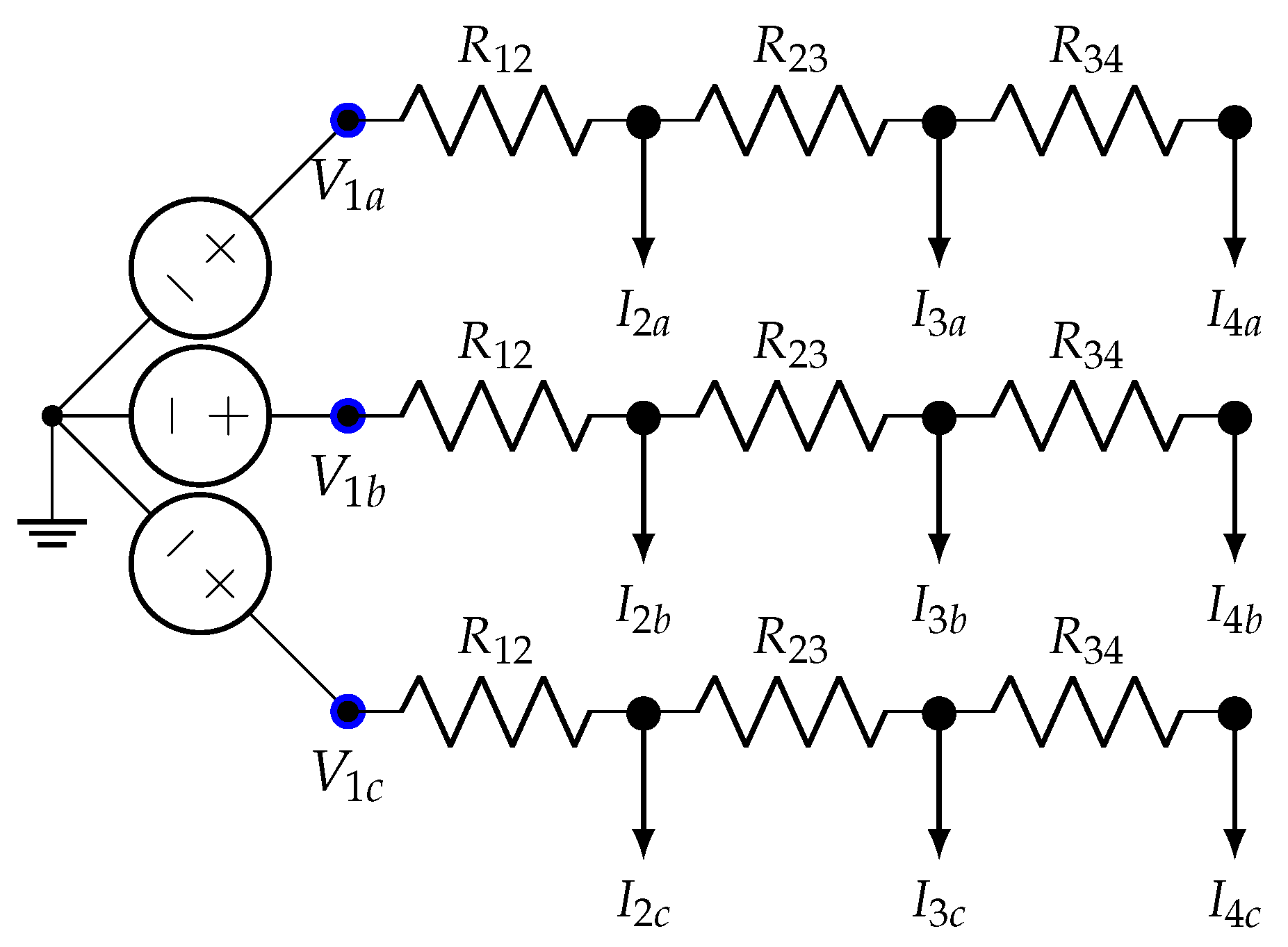
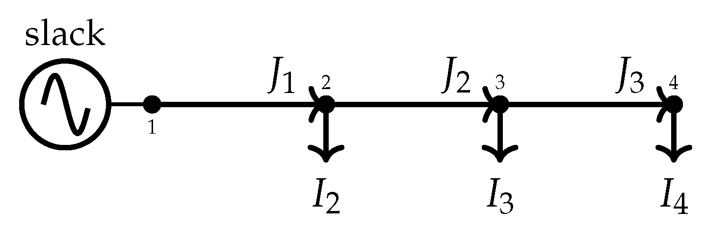
3.1. Three-Phase Power Flow
| Algorithm 1: Generic solution of the power flow problem in three-phase unbalanced distribution networks using the triangular formulation |
 |
3.2. Overall Solution Methodology
| Algorithm 2: Optimal load redistribution in DS using a mixed-integer convex model based on electrical momentum |
|
Data: Define the distribution system under study 1 Solve the initial three-phase power flow problem using Algorithm 1; 2 Report the initial power losses; 3 Program the MIQC model based on the electrical moment with Equations (1)–(7) in the GAMS software; 4 Solve the MIQC model using a convex optimization tool; 5 Redistribute all of the demanded loads based on the solution provided by the MIQC solution; 6 Solve the final three-phase power flow problem using Algorithm 1; 7 Report the final power losses; 8 Compare the effect of the optimal load redistribution on the total grid power losses; |
4. Test System
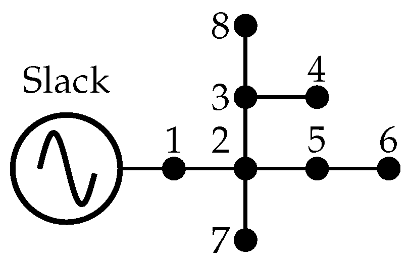
4.1. 8-Bus Test System
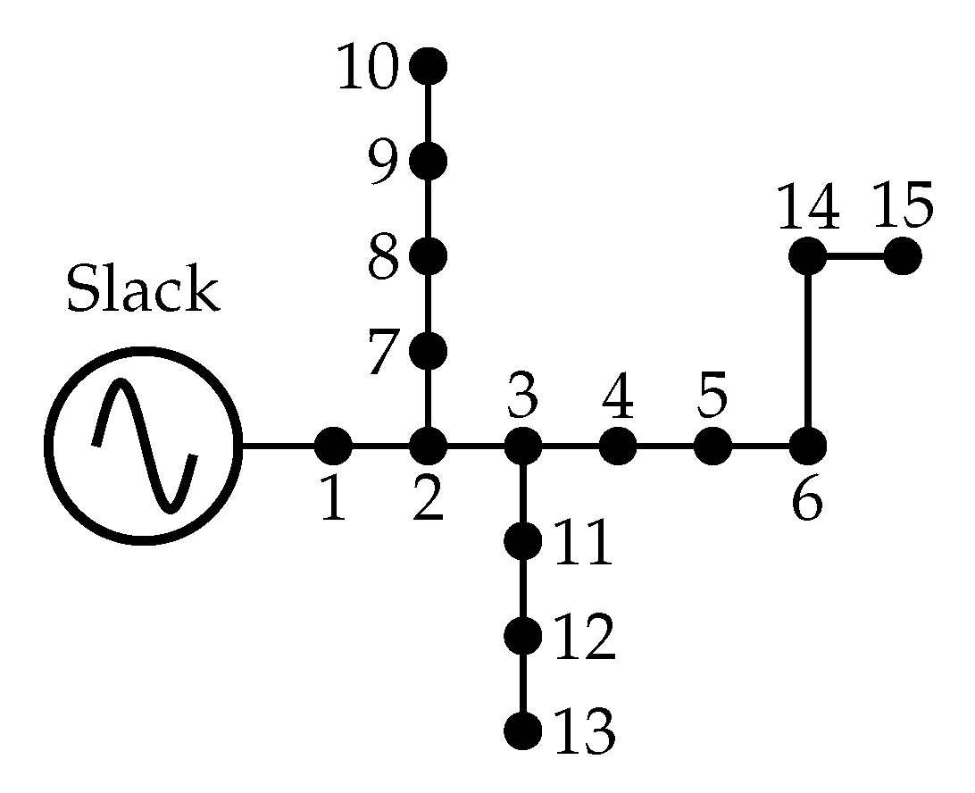
4.2. 15-Bus Test System
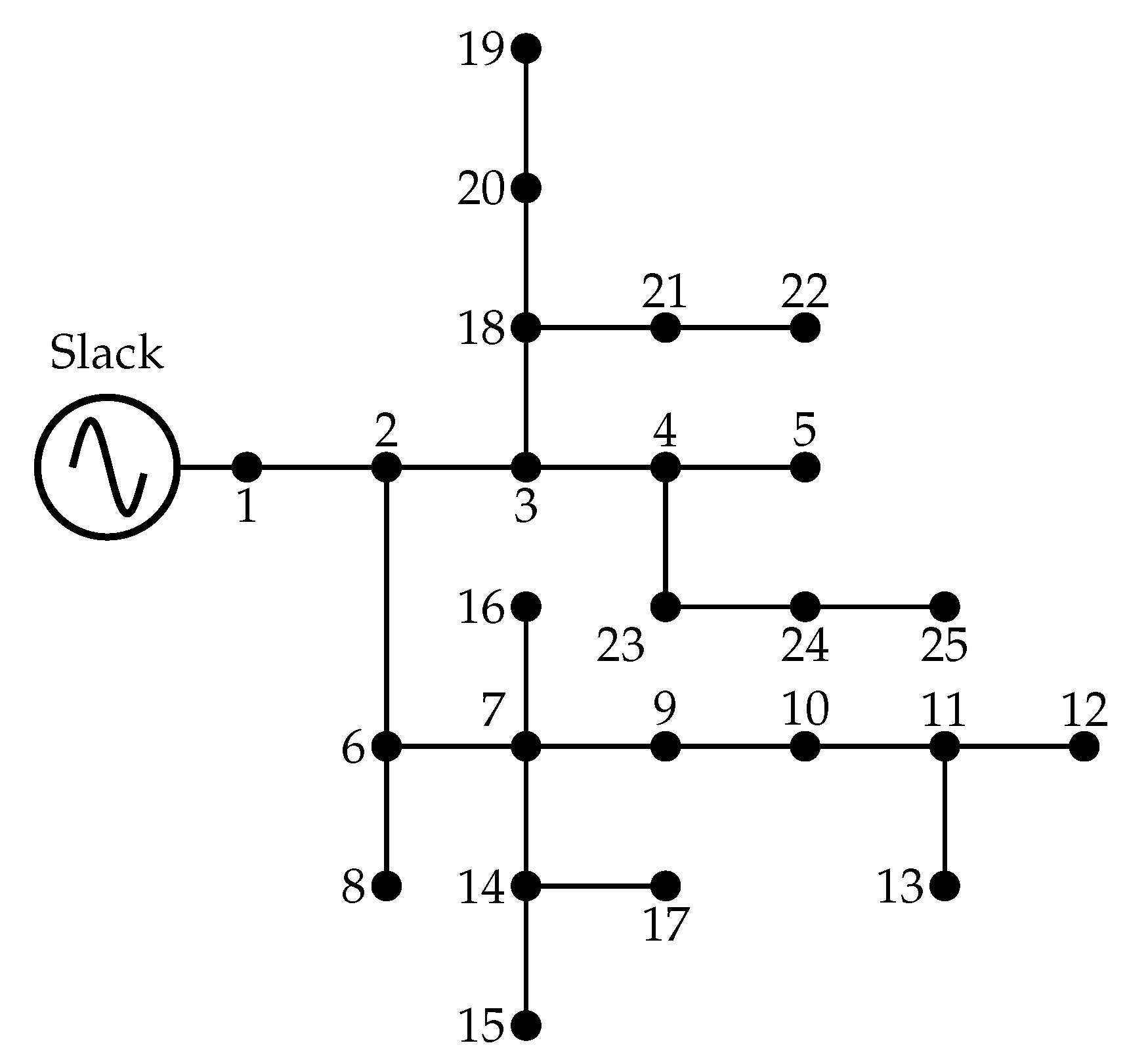
4.3. 25-Bus Test System
5. Results Analysis
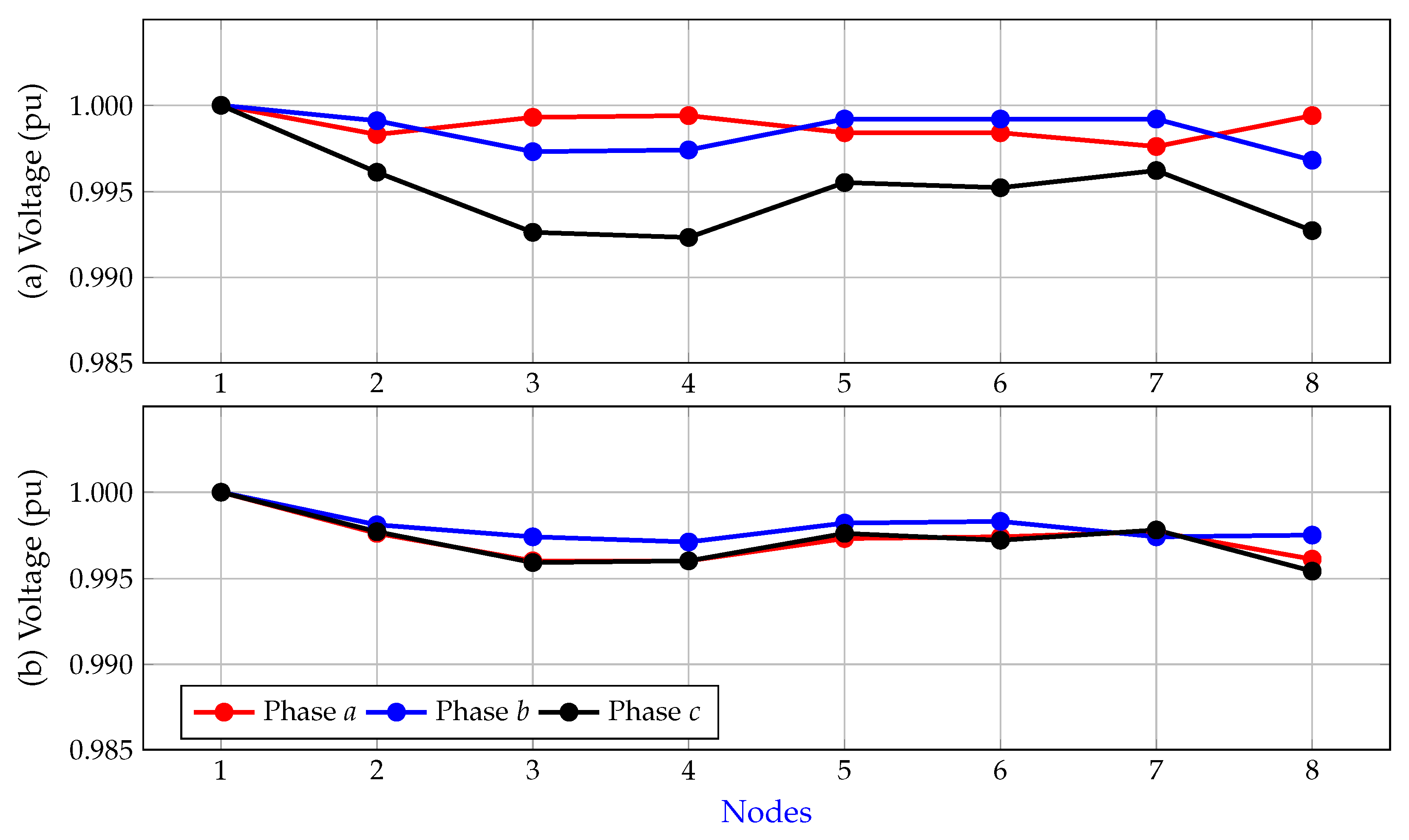
5.1. 8-Bus System
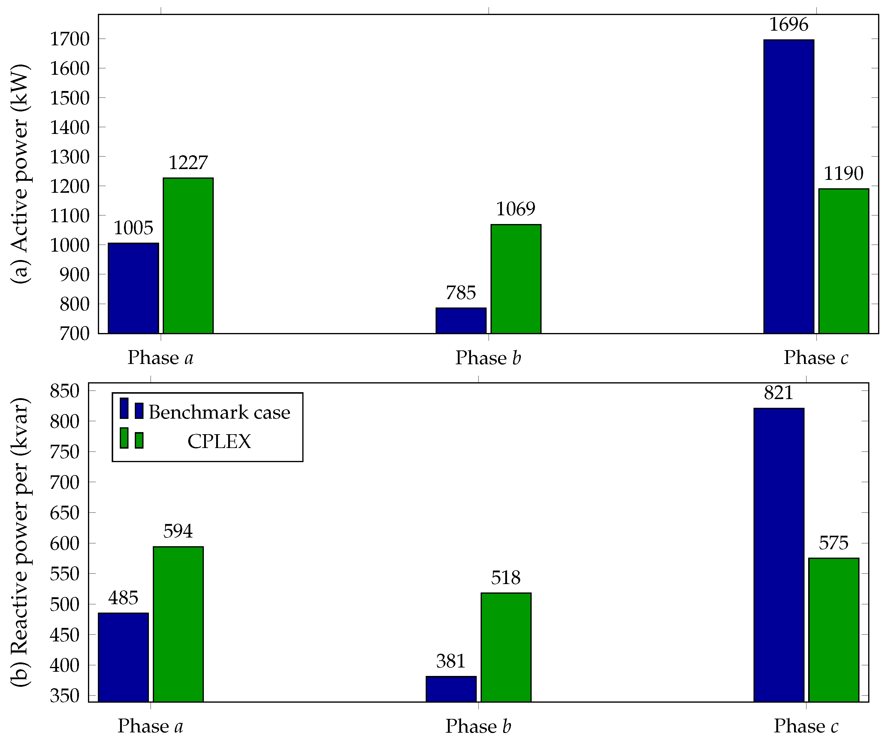
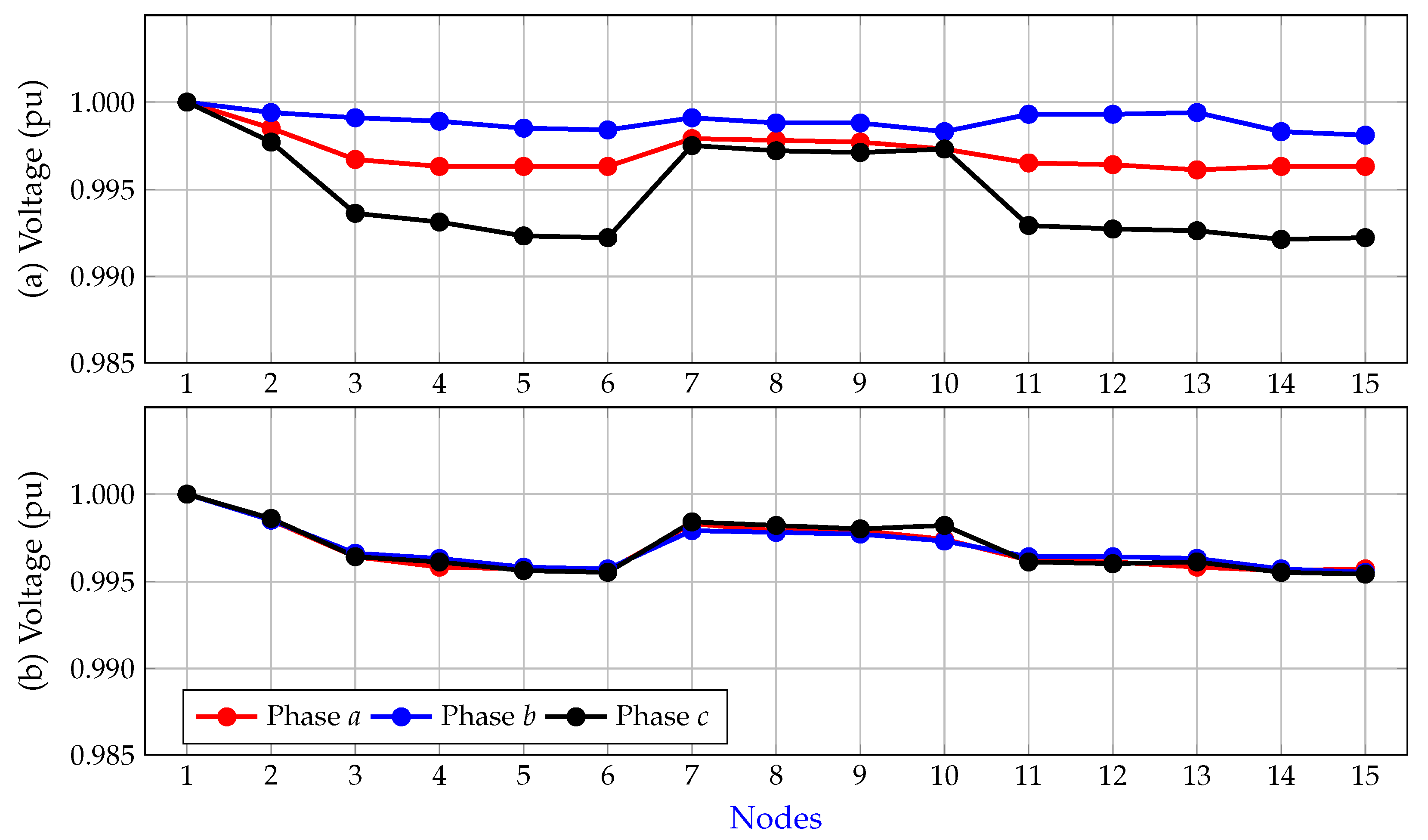
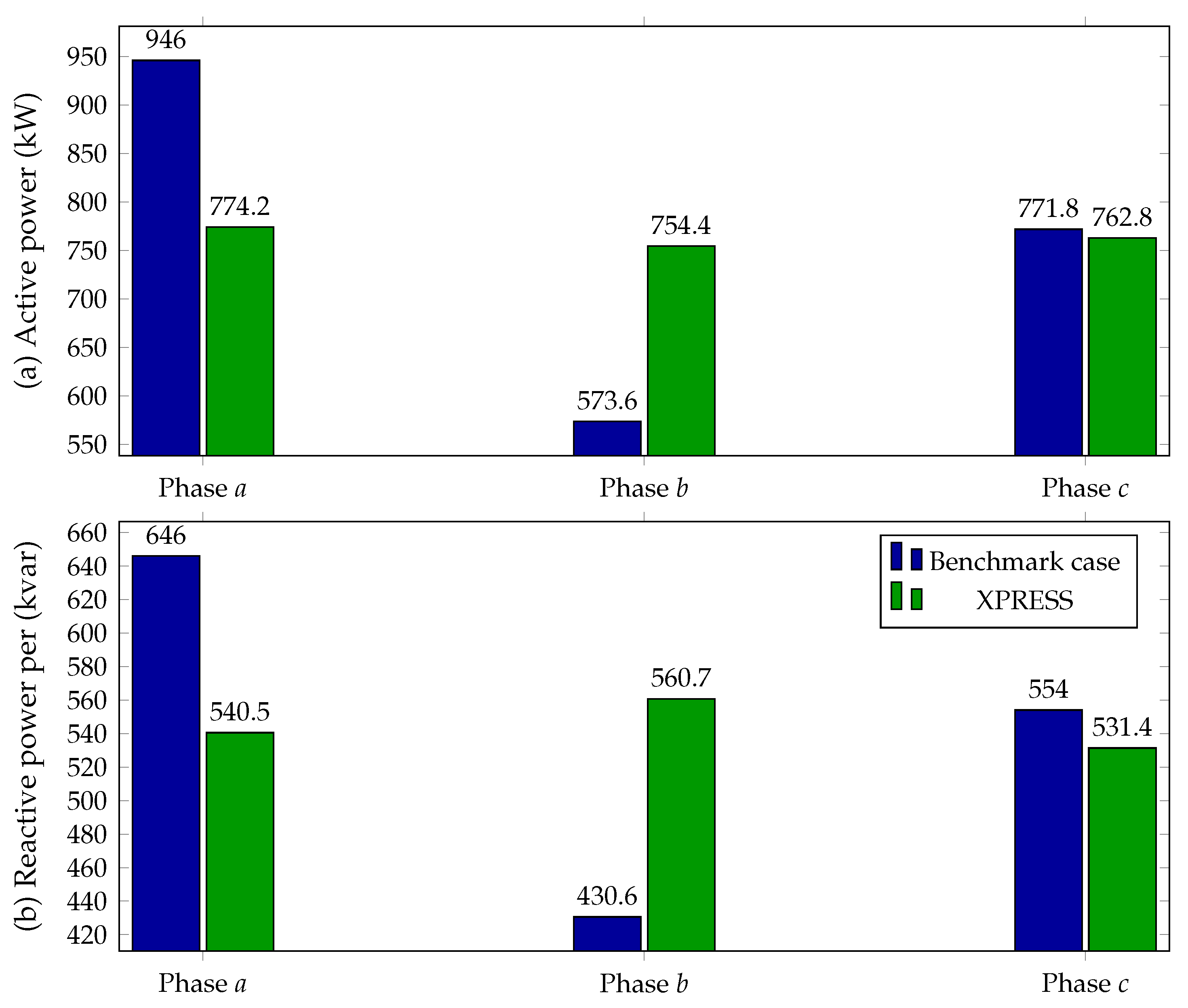
5.2. 15-Bus System
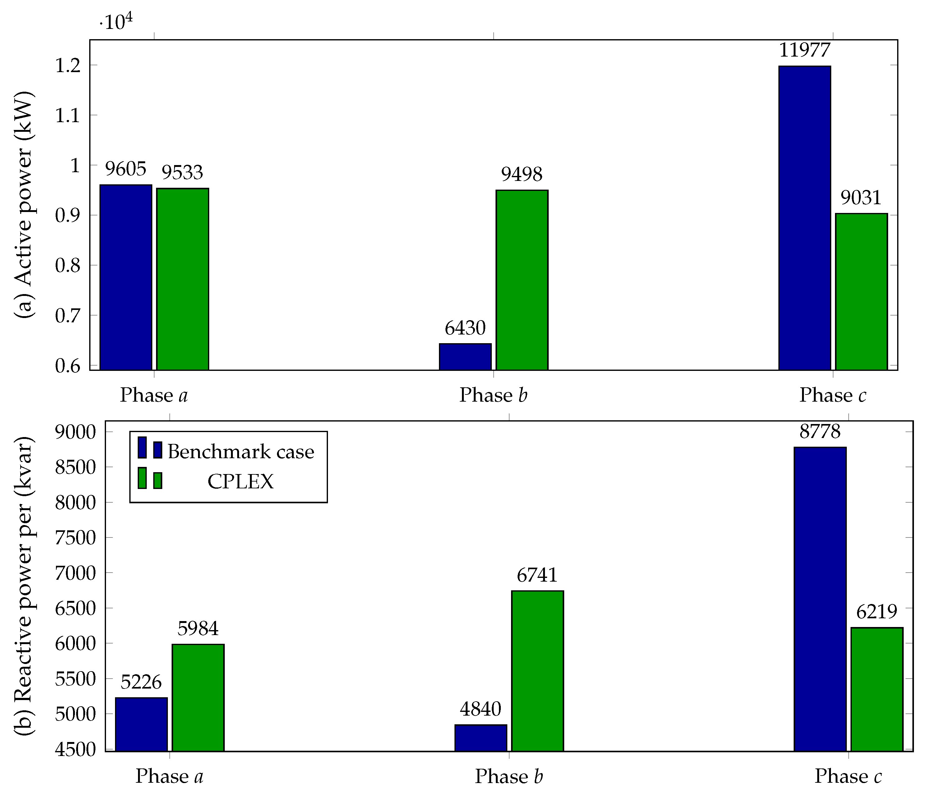
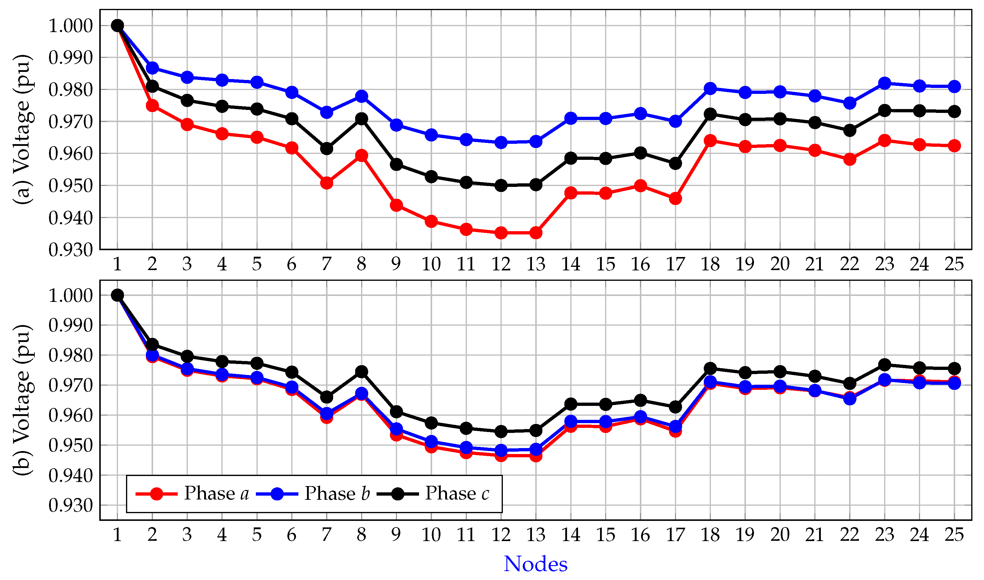
5.3. 25-Bus System
6. Conclusions and Future Works
Author Contributions
Funding
Institutional Review Board Statement
Informed Consent Statement
Data Availability Statement
Acknowledgments
Conflicts of Interest
Nomenclature
| Acronyms | |
| BHO | Black hole optimizer. |
| CPLEX | Solver available in GAMS for MIQC models. |
| DS | Distribution system. |
| DSO | Distribution system operator. |
| GAMS | General algebraic modeling system. |
| MIQC | Mixed-integer quadratic convex. |
| MIQC-AI | Mixed-integer quadratic convex model based on average current. |
| MIQC-AP | Mixed-integer quadratic convex model based on average power. |
| MIQC-EM | Mixed-integer quadratic convex model based on electrical momentum. |
| SBB | Solver available in GAMS for MIQC models. |
| SCA | Sine-cosine algorithm. |
| XPRESS | Solver available in GAMS for MIQC models. |
| Parameters | |
| Three-phase upper-triangular matrix. | |
| Primitive impedance matrix that contains the three-phase impedances of the branches (). | |
| Active power consumed at node k in phase f before load redistribution (W). | |
| Reactive power consumed at node k in phase f before load redistribution (var). | |
| Average value of the resistance of the three-phase line (). | |
| Position of the upper-triangular matrix that relates line l with node k. | |
| Three-phase voltage at the substation node (V). | |
| Sets | |
| Set containing all phases of the distribution network. | |
| Set containing all the three-phase distribution lines. | |
| Set containing all of the three-phase nodes. | |
| Variables | |
| Vector that contains all of the three-phase voltage drops in each of the branches in the complex domain (V). | |
| Vector containing all of the three-phase demanded currents at the nodes of the network except the slack node (A). | |
| Vector that contains all of the three-phase branch currents in the complex domain (A). | |
| Vector that contains all of the three-phase voltage in the demand nodes except the slack source (V). | |
| Active power consumed after load redistribution at node k for phase f (W). | |
| Active power flow in line l in phase f (W). | |
| Active power accumulated downstream which impacts line l (W). | |
| Reactive power consumed after load redistribution at node k for phase f (var). | |
| Reactive power flow in line l in phase f (var). | |
| Reactive power accumulated downstream which impacts line l (var). | |
| Binary variable (matrix) that determines whether the load connected in phase g should be reassigned to phase f at node k. | |
| z | Objective function value (-(VA)). |
| Equivalent apparent power losses of the three-phase unbalanced network (VA). | |
References
- CREG. Resolución CREG 015 de 2018: By which the Methodology for the Remuneration of the Electricity Distribution Activity in the National Interconnected System; Technical Report; Gobierno de Colombia: Bogotá, Colombia, 2018. (In Spanish)
- Montoya, O.D.; Giraldo, J.S.; Grisales-Noreña, L.F.; Chamorro, H.R.; Alvarado-Barrios, L. Accurate and Efficient Derivative-Free Three-Phase Power Flow Method for Unbalanced Distribution Networks. Computation 2021, 9, 61. [Google Scholar] [CrossRef]
- Montoya, O.D.; Arias-Londoño, A.; Grisales-Noreña, L.F.; Barrios, J.Á.; Chamorro, H.R. Optimal Demand Reconfiguration in Three-Phase Distribution Grids Using an MI-Convex Model. Symmetry 2021, 13, 1124. [Google Scholar] [CrossRef]
- Alhmoud, L.; Nawafleh, Q.; Merrji, W. Three-Phase Feeder Load Balancing Based Optimized Neural Network Using Smart Meters. Symmetry 2021, 13, 2195. [Google Scholar] [CrossRef]
- Cavalheiro, E.M.B.; Lyra, C. Optimal Configuration of Power Distribution Networks with Small Intermittent Energy Sources. In Proceedings of the 2019 IEEE PES Innovative Smart Grid Technologies Conference—Latin America (ISGT Latin America), Gramado, Brazil, 15–18 September 2019. [Google Scholar] [CrossRef]
- Massaferro, P.; Martino, J.M.D.; Fernandez, A. Fraud Detection in Electric Power Distribution: An Approach That Maximizes the Economic Return. IEEE Trans. Power Syst. 2020, 35, 703–710. [Google Scholar] [CrossRef]
- Cortés-Caicedo, B.; Avellaneda-Gómez, L.S.; Montoya, O.D.; Alvarado-Barrios, L.; Chamorro, H.R. Application of the Vortex Search Algorithm to the Phase-Balancing Problem in Distribution Systems. Energies 2021, 14, 1282. [Google Scholar] [CrossRef]
- Montoya, O.D.; Alarcon-Villamil, J.A.; Hernández, J.C. Operating cost reduction in distribution networks based on the optimal phase-swapping including the costs of the working groups and energy losses. Energies 2021, 14, 4535. [Google Scholar] [CrossRef]
- Kong, W.; Ma, K.; Fang, L.; Wei, R.; Li, F. Cost-Benefit Analysis of Phase Balancing Solution for Data-Scarce LV Networks by Cluster-Wise Gaussian Process Regression. IEEE Trans. Power Syst. 2020, 35, 3170–3180. [Google Scholar] [CrossRef]
- Malmedal, K.; Sen, P.K. A Better Understanding of Load and Loss Factors. In Proceedings of the 2008 IEEE Industry Applications Society Annual Meeting, Edmonton, AB, Canada, 5–9 October 2008. [Google Scholar] [CrossRef]
- Garces, A.; Gil-González, W.; Montoya, O.D.; Chamorro, H.R.; Alvarado-Barrios, L. A Mixed-Integer Quadratic Formulation of the Phase-Balancing Problem in Residential Microgrids. Appl. Sci. 2021, 11, 1972. [Google Scholar] [CrossRef]
- Cadena, R.H. Central System Metering on Low Voltage Utility Distribution Networks to Reduce the Energy Loss. In Simposio Internacional sobre la Calidad de la Energía Eléctrica—SICEL; Universidad Nacional de Colombia: Bogota, Colombia, 2017; Volume 9. [Google Scholar]
- Al-Kharsan, I.; Marhoon, A.; Mahmood, J. Phase Swapping Load Balancing Algorithms, Comprehensive Survey. Iraqi J. Electr. Electron. Eng. 2019, 15, 40–49. [Google Scholar] [CrossRef]
- Aljendy, R.I.; Nasyrov, R.R.; Sultan, H.M.; Diab, A.A.Z. Bio-inspired Optimization Techniques for Compensation Reactive Power and Voltage Profile Improvement in the Syrian Electrical Distribution Systems. In Proceedings of the 2019 IEEE Conference of Russian Young Researchers in Electrical and Electronic Engineering (EIConRus), Saint Petersburg and Moscow, Russia, 28–31 January 2019. [Google Scholar] [CrossRef]
- Kaur, M.; Ghosh, S. Network reconfiguration of unbalanced distribution networks using fuzzy-firefly algorithm. Appl. Soft Comput. 2016, 49, 868–886. [Google Scholar] [CrossRef]
- Bao, G.; Ke, S. Load Transfer Device for Solving a Three-Phase Unbalance Problem Under a Low-Voltage Distribution Network. Energies 2019, 12, 2842. [Google Scholar] [CrossRef]
- Aguila, A.; Wilson, J. Technical and Economic Assessment of the Implementation of Measures for Reducing Energy Losses in Distribution Systems. IOP Conf. Ser. Earth Environ. Sci. 2017, 73, 012018. [Google Scholar] [CrossRef]
- Ismael, S.M.; Aleem, S.H.E.A.; Abdelaziz, A.Y. Optimal selection of conductors in Egyptian radial distribution systems using sine–cosine optimization algorithm. In Proceedings of the 2017 Nineteenth International Middle East Power Systems Conference (MEPCON), Cairo, Egypt, 19–21 December 2017. [Google Scholar] [CrossRef]
- Esmaeili, S.; Anvari-Moghaddam, A.; Jadid, S.; Guerrero, J. A Stochastic Model Predictive Control Approach for Joint Operational Scheduling and Hourly Reconfiguration of Distribution Systems. Energies 2018, 11, 1884. [Google Scholar] [CrossRef]
- Flaih, F.; Lin, X.; Abd, M.; Dawoud, S.; Li, Z.; Adio, O. A New Method for Distribution Network Reconfiguration Analysis under Different Load Demands. Energies 2017, 10, 455. [Google Scholar] [CrossRef]
- Nguyen, T.T.; Nguyen, Q.T.; Nguyen, T.T. Optimal radial topology of electric unbalanced and balanced distribution system using improved coyote optimization algorithm for power loss reduction. Neural Comput. Appl. 2021, 33, 12209–12236. [Google Scholar] [CrossRef]
- Jakus, D.; Čađenović, R.; Vasilj, J.; Sarajčev, P. Optimal Reconfiguration of Distribution Networks Using Hybrid Heuristic-Genetic Algorithm. Energies 2020, 13, 1544. [Google Scholar] [CrossRef]
- Zhai, H.; Yang, M.; Chen, B.; Kang, N. Dynamic reconfiguration of three-phase unbalanced distribution networks. Int. J. Electr. Power Energy Syst. 2018, 99, 1–10. [Google Scholar] [CrossRef]
- Borges, M.C.O.; Franco, J.F.; Rider, M.J. Optimal Reconfiguration of Electrical Distribution Systems Using Mathematical Programming. J. Control. Autom. Electr. Syst. 2013, 25, 103–111. [Google Scholar] [CrossRef]
- Ehsan, A.; Yang, Q. Optimal integration and planning of renewable distributed generation in the power distribution networks: A review of analytical techniques. Appl. Energy 2018, 210, 44–59. [Google Scholar] [CrossRef]
- Zheng, W.; Huang, W.; Hill, D.J.; Hou, Y. An Adaptive Distributionally Robust Model for Three-Phase Distribution Network Reconfiguration. IEEE Trans. Smart Grid 2021, 12, 1224–1237. [Google Scholar] [CrossRef]
- Wang, W.; Yu, N. Maximum Marginal Likelihood Estimation of Phase Connections in Power Distribution Systems. IEEE Trans. Power Syst. 2020, 35, 3906–3917. [Google Scholar] [CrossRef]
- Rios, M.A.; Castano, J.C.; Garces, A.; Molina-Cabrera, A. Phase Balancing in Power Distribution Systems: A heuristic approach based on group-theory. In Proceedings of the 2019 IEEE Milan PowerTech, Milan, Italy, 23–27 June 2019. [Google Scholar] [CrossRef]
- Kazemi-Robati, E.; Sepasian, M.S. Fast heuristic methods for harmonic minimization using distribution system reconfiguration. Electr. Power Syst. Res. 2020, 181, 106185. [Google Scholar] [CrossRef]
- Siti, W.; Jimoh, A.; Nicolae, D. Phase Load Balancing in the Secondary Distribution Network Using a Fuzzy Logic and a Combinatorial Optimization Based on the Newton Raphson. In Intelligent Data Engineering and Automated Learning—IDEAL 2009; Springer: Berlin/Heidelberg, Germany, 2009; pp. 92–100. [Google Scholar] [CrossRef]
- Schweickardt, G.; Miranda, V. Metaheuristics FEPSO Applied to Combinatorial Optimization: Phase Balancing in Electric Distributions Systems. Cienc. Docencia Tecnol. 2010, 21, 133–163. (In Spanish) [Google Scholar]
- Al-Kharsan, I.H. A new strategy for phase swapping load balancing relying on a metaheuristic MOGWO algorithm. J. Mech. Contin. Math. Sci. 2020, 15, 84–102. [Google Scholar] [CrossRef]
- Montoya, O.D.; Grisales-Noreña, L.F.; Rivas-Trujillo, E. Approximated Mixed-Integer Convex Model for Phase Balancing in Three-Phase Electric Networks. Computers 2021, 10, 109. [Google Scholar] [CrossRef]
- Kong, W.; Ma, K.; Wu, Q. Three-Phase Power Imbalance Decomposition Into Systematic Imbalance and Random Imbalance. IEEE Trans. Power Syst. 2018, 33, 3001–3012. [Google Scholar] [CrossRef]
- Ravindran, A.; Ragsdell, K.M.; Reklaitis, G.V. Engineering Optimization; John Wiley & Sons, Inc.: Hoboken, NJ, USA, 2006. [Google Scholar] [CrossRef]
- Giraldo, J.S.; Vergara, P.P.; Lopez, J.C.; Nguyen, P.H.; Paterakis, N.G. A Novel Linear Optimal Power Flow Model for Three-Phase Electrical Distribution Systems. In Proceedings of the 2020 International Conference on Smart Energy Systems and Technologies (SEST), Istanbul, Turkey, 7–9 September 2020. [Google Scholar] [CrossRef]
- Marini, A.; Mortazavi, S.; Piegari, L.; Ghazizadeh, M.S. An efficient graph-based power flow algorithm for electrical distribution systems with a comprehensive modeling of distributed generations. Electr. Power Syst. Res. 2019, 170, 229–243. [Google Scholar] [CrossRef]
- Shen, T.; Li, Y.; Xiang, J. A Graph-Based Power Flow Method for Balanced Distribution Systems. Energies 2018, 11, 511. [Google Scholar] [CrossRef]
- Soroudi, A. Power System Optimization Modeling in GAMS; Springer International Publishing: Berlin/Heidelberg, Germany, 2017. [Google Scholar] [CrossRef]


| Solution Methodology | Objective Function | Ref. | Year |
|---|---|---|---|
| Fuzzy logic combined with the Newton–Raphson method | Power losses minimization | [30] | 2009 |
| Fuzzy evolutionary particle swarm optimization | Power losses minimization | [31] | 2010 |
| Quadratic optimization model | Voltage imbalance minimization | [34] | 2017 |
| Multi-objective genetic algorithm | Voltage imbalance and switching actions minimization | [16] | 2019 |
| Multi-objective gray wolf optimizer | Voltage imbalance and power losses minimization | [32] | 2020 |
| Birkhoff polytope | Reducing the expected value of active power losses | [11] | 2021 |
| Artificial neural networks and smart meters | Energy losses minimization | [4] | 2021 |
| Mixed-integer convex optimization approach based on the average current | Power losses minimization | [33] | 2021 |
| Mixed-integer convex optimization approach based on the average power | Power losses minimization | [3] | 2021 |
| Vortex search algorithm | Power losses minimization | [7] | 2021 |
| Sine-cosine algorithm | Power losses minimization | [8] | 2021 |
| Option 0 | Option 1 | Option 2 | ||||||||
|---|---|---|---|---|---|---|---|---|---|---|
| Route i–j | (A) | (A) | (A) | (A) | (A) | (A) | (A) | (A) | (A) | |
| 1–2 | 0.035 | 20 | 20 | 15 | 20 | 20 | 15 | 20 | 15 | 20 |
| 2–3 | 0.025 | 15 | 20 | 10 | 15 | 10 | 20 | 15 | 10 | 20 |
| 3–4 | 0.040 | 15 | 25 | 0 | 15 | 25 | 0 | 15 | 25 | 0 |
| Electrical momentum | (W) | (W) | (W) | |||||||
| Type of Connection | Phases | Sequence | Binary Variable () |
|---|---|---|---|
| 1 | ABC | ||
| 2 | CAB | No change | |
| 3 | BCA | ||
| 4 | ACB | ||
| 5 | BAC | Change | |
| 6 | CBA |
| Method | Connections | Active Losses (kW) | Reduction (%) |
|---|---|---|---|
| Benchmark case | 13.9925 | - | |
| CPLEX | 10.5869 | 24.34 | |
| SBB | 10.8413 | 22.52 | |
| XPRESS | 10.5869 | 24.34 |
| Method | Power Losses (kW) | Reduction (%) |
|---|---|---|
| Benchmark case | 13.9925 | - |
| BHO | 10.5869 | 24.34 |
| SCA | 10.5869 | 24.34 |
| MIQC-AP [3] | 10.7613 | 23.09 |
| MIQC-AI [33] | 10.5869 | 24.34 |
| MIQC-EM | 10.5869 | 24.34 |
| Method | Connections | Active Losses (kW) | Reduction (%) |
|---|---|---|---|
| Benchmark case | 134.2472 | - | |
| CPLEX | 109.2218 | 22.05 | |
| SBB | 110.3654 | 17.79 | |
| XPRESS | 109.3706 | 18.53 |
| Method | Power Losses (kW) | Reduction (%) |
|---|---|---|
| Benchmark case | 134.2472 | - |
| BHO | 110.0025 | 18.06 |
| SCA | 109.3973 | 18.51 |
| MIQC-AP [3] | 110.7776 | 17.48 |
| MIQC-AI [33] | 109.2539 | 18.62 |
| MIQC-EM | 109.2218 | 18.64 |
| Method | Connections | Active Losses (kW) | Reduction (%) |
|---|---|---|---|
| BENCHMARK | 75.4206 | - | |
| CPLEX | 72.3103 | 4.12 | |
| SBB | 72.3630 | 4.05 | |
| XPRESS | 72.3017 | 4.14 |
Disclaimer/Publisher’s Note: The statements, opinions and data contained in all publications are solely those of the individual author(s) and contributor(s) and not of MDPI and/or the editor(s). MDPI and/or the editor(s) disclaim responsibility for any injury to people or property resulting from any ideas, methods, instructions or products referred to in the content. |
© 2023 by the authors. Licensee MDPI, Basel, Switzerland. This article is an open access article distributed under the terms and conditions of the Creative Commons Attribution (CC BY) license (https://creativecommons.org/licenses/by/4.0/).
Share and Cite
Bohórquez-Álvarez, D.P.; Niño-Perdomo, K.D.; Montoya, O.D. Optimal Load Redistribution in Distribution Systems Using a Mixed-Integer Convex Model Based on Electrical Momentum. Information 2023, 14, 229. https://doi.org/10.3390/info14040229
Bohórquez-Álvarez DP, Niño-Perdomo KD, Montoya OD. Optimal Load Redistribution in Distribution Systems Using a Mixed-Integer Convex Model Based on Electrical Momentum. Information. 2023; 14(4):229. https://doi.org/10.3390/info14040229
Chicago/Turabian StyleBohórquez-Álvarez, Daniela Patricia, Karen Dayanna Niño-Perdomo, and Oscar Danilo Montoya. 2023. "Optimal Load Redistribution in Distribution Systems Using a Mixed-Integer Convex Model Based on Electrical Momentum" Information 14, no. 4: 229. https://doi.org/10.3390/info14040229
APA StyleBohórquez-Álvarez, D. P., Niño-Perdomo, K. D., & Montoya, O. D. (2023). Optimal Load Redistribution in Distribution Systems Using a Mixed-Integer Convex Model Based on Electrical Momentum. Information, 14(4), 229. https://doi.org/10.3390/info14040229