Graph Neural Networks and Open-Government Data to Forecast Traffic Flow

Abstract

Traffic forecasting has been an important area of research for several decades, with significant implications for urban traffic planning, management, and control. In recent years, deep-learning models, such as graph neural networks (GNN), have shown great promise in traffic forecasting due to their ability to capture complex spatio–temporal dependencies within traffic networks. Additionally, public authorities around the world have started providing real-time traffic data as open-government data (OGD). This large volume of dynamic and high-value data can open new avenues for creating innovative algorithms, services, and applications. In this paper, we investigate the use of traffic OGD with advanced deep-learning algorithms. Specifically, we deploy two GNN models—the Temporal Graph Convolutional Network and Diffusion Convolutional Recurrent Neural Network—to predict traffic flow based on real-time traffic OGD. Our evaluation of the forecasting models shows that both GNN models outperform the two baseline models—Historical Average and Autoregressive Integrated Moving Average—in terms of prediction performance. We anticipate that the exploitation of OGD in deep-learning scenarios will contribute to the development of more robust and reliable traffic-forecasting algorithms, as well as provide innovative and efficient public services for citizens and businesses.

1. Introduction

Traffic forecasting, which is an important component of intelligent transportation systems, assists policymakers and public authorities to design and manage transportation systems that are efficient, safe, environmentally friendly, and cost-effective [1]. Traffic forecasts can be used to anticipate future needs and allocate resources accordingly, such as managing traffic lights [2,3], opening or closing lanes, estimating travel time [4], and mitigating traffic congestion [5,6,7]. The prediction of future traffic states based on historical or real-time traffic data can contribute to reducing the impact of negative effects on citizens such as health problems brought on by air pollution, and economic costs such as increased travel time spent, and wasted fuels, with a detrimental effect on both the environment and the quality of citizens’ lives [8,9,10,11].

However, traffic forecasting is a challenging field due to the complex spatio–temporal dependencies that occur in the road network. Literature usually exploits three types of techniques to forecast future traffic conditions based on historical observations of traffic data; (i) traditional parametric methods including stochastic and temporal methods (e.g., Autoregressive Integrated Moving Average—ARIMA [12]); (ii) machine learning (e.g., Support Vector Machine [5]); and (iii) deep learning [11,13,14,15]. Artificial Intelligence approaches outperform parametric approaches due to their ability to deal with large quantities of data [16,17]. In addition, the parametric models fail to provide accurate results due to the stochastic and non-linear nature of traffic flow [18].

Recently, a significant number of research papers have explored the effectiveness of deep-learning algorithms on urban traffic forecasting, especially graph neural networks (GNNs) (e.g., [19,20,21,22]). These models manage to capture the complex topology of a road network, by extending the convolution operation from Euclidean to non-Euclidean space, while dynamic temporal dependencies are captured by the integration of recurrent units.

The rapid development of the Internet of Things (IoT) can significantly facilitate traffic forecasting by providing data sources (e.g., sensors), which generate large quantities of traffic data that can be analyzed to forecast the volume and density of traffic flow. Dynamic (or real-time) data with traffic-related information (e.g., counted number of vehicles, average speed) that are generated by sensors have only recently started being provided as open-government data (OGD) [23,24,25] available for free access and reuse. Dynamic OGD are suitable for creating value-added services, applications and high-quality and decent jobs, and are, hence, characterized as high-value data (HVD), with substantial societal, environmental, and financial advantages [26]. However, collecting and reusing this type of data requires addressing various challenges. For example, dynamic data are known for their high variability and quick obsolescence and should, hence, be immediately available and regularly updated to develop added-value services and applications. In addition, a recent work [27] showed that dynamic traffic data confront major quality challenges. These challenges are often caused by sensor malfunctions, e.g., brought on by bad climatic conditions [28].

This paper aims to investigate the exploitation of traffic OGD using state-of-the-art deep-learning algorithms. Specifically, we use two widely used and open-source GNN algorithms, namely Temporal Graph Convolutional Network (TGCN) and Diffusion Convolutional Recurrent Neural Network (DCRNN), and real-time traffic data from the Greek open-data portal to create models that accurately forecast traffic flow. The models forecast traffic flow in three time horizons, i.e., in the next 3 (short-term prediction), 6 (middle-term prediction), and 9 (long-term prediction) time steps (hours). The Greek data portal was selected for this work since it provides an Application Programming Interface (API) to access traffic data. We anticipate that the exploitation of OGD in deep-learning scenarios will contribute towards both (a) the development of more robust and reliable traffic-forecasting deep-learning algorithms and (b) the provision of innovative and efficient public services to citizens and businesses alike.

The rest of this paper is organized as follows. Section 2 presents related work describing traffic-forecasting, deep-learning approaches, and graph neural networks for traffic forecasting. Section 3 presents background knowledge regarding the two GNN algorithms employed in this work. Thereafter, Section 4 describes in detail the specific steps followed in this research. In addition, Section 5 and Section 6 present the case study by first describing the collection of the traffic data from the Greek open-data portal (Section 5), and the pre-processing of the traffic data (Section 6), and then the creation and evaluation of the forecasting model (Section 7). Finally, Section 8 discusses the results of this paper and Section 9 concludes this paper.

2. Related Work

This section presents a review of the previous work in traffic forecasting, deep-learning approaches, and graph neural networks for traffic forecasting to facilitate readers’ quick understanding of the key aspects of this work.

2.1. Traffic Forecasting

Intelligent Transportation Systems (ITS) aim to improve the operational efficiency of transportation networks by gathering, processing and analyzing massive amounts of traffic information [29]. This information is produced by sensors (e.g., loop detectors), traffic surveillance videos or Bluetooth devices that are in several control points of the transportation network such as roadways, highways, terminals, etc. In the rapid development of intelligent transportation systems, traffic forecasting has been considered a very important and developing area for both research and business applications, with a large range of published articles in the field [30,31]. Traffic forecasting is the process of estimating future traffic states given a continuum of historical traffic data. Moreover, it is one of the most challenging tasks among other time-series prediction problems because it involves huge amounts of data that have both complex spatial and temporal dependencies. In the context of traffic-forecasting problems, spatial dependencies of traffic time series, refer to the topological information of the transportation network and its effects on adjacent or distant traffic measurement points [32]. For instance, the traffic state in a particular location may (or not) be affected by traffic on nearby roads. Furthermore, complex temporal dynamics may include seasonality, periodicity, trend and other unexpected random events that may occur in a transportation network, such as accidents, construction sites and weather.

Data-driven traffic-forecasting modeling has been at the center of transportation research activity and efforts during the last three decades [1]. Most of the existing literature focuses on the prediction of three main traffic states, namely traffic flow (vehicles/time unit), average speed, and density (vehicles/distance). Many existing forecasting methods consider temporal dependence based on classic statistics such as Autoregressive Integrated Moving Average and its variants [33], and more complex machine-learning methods including Support Vector regression machine method [34], K-nearest neighbor models [35,36], and Bayesian networks [37]. Although both statistical and machine-learning models effectively consider the dynamic temporal features of past traffic conditions, they fail to extract spatial dependence.

2.2. Deep-Learning Approaches

Recently, the emerging development of deep-learning and neural networks has achieved significant success in traffic-forecasting tasks [13,14]. To model the temporal non-linear dependency, researchers proposed Recurrent Neural Networks (RNN) and their variants. RNNs are deep neural network models that manage to adapt sequential data but suffer from exploding and vanishing gradients during back propagation [38]. To mitigate these effects during training of such models, numerous research studies proposed alternative architectures based on RNNs, such as Long Short Memory networks (LSTM) and Gated Recurrent Units (GRU) [39,40,41]. These variants of RNNs use gated mechanisms to memorize long-term dependencies in sequence-based data including historical traffic information [42]. Their structure consists of various forget units that determine which information could be excluded from the prediction output, thus determining the optimal time windows [40]. GRUs are similar architectures to LSTMs, but they have a simpler structure being computationally efficient during training and their cells consist of two main gates, namely the reset gate and the update gate [40]. Similar to the traditional statistical and machine-learning models, the recurrent-based models ignore the spatial information that is hidden in traffic data, failing to adapt the road network topology. To this end, many research efforts focused on improving the prediction accuracy by considering temporal, as well as spatial features. An approach to capture the spatial relations among the traffic network is the use of convolutional neural networks (CNNs) combined with recurrent neural networks (RNN) for temporal modeling. For example, Ref. [43] proposed a 1-dimension CNN to capture spatial information of traffic flow combined with two LSTMs to adapt short-term variability and various periodicities of traffic flow. Another attempt to align spatial and temporal patterns is made by [44], proposing a convolutional LSTM that models a spatial region with a grid, extending the convolution operations applied on grid structures (e.g., images). Furthermore, Ref. [45] deployed deep convolutional networks to capture spatial relationships among traffic links. In this study the network topology is represented by a grid box, where near and far dependencies are captured at each convolutional operation. These spatial convolutions are then combined with LSTM networks that adapt temporal information.

In recent years, a significant amount of research papers have focused on embedding spatial information into traffic-forecasting models [14,21]. However, methods that use convolutional neural networks (CNNs) are limited to cases where the data have a Euclidean structure, thus they cannot fully capture the complex topological structure of transportation networks, such as subways or road networks. Graph Neural Networks (GNNs) have become the frontier of deep-learning research in graph representation learning, demonstrating state-of-the-art performance in a variety of applications [46]. They can effectively model spatial dependencies that are represented by non-Euclidean graph structures. To this end, they are ideally suited for traffic-forecasting problems because a road network can be naturally represented as a graph, with intersections modeled as graph nodes and roads as edges.

2.3. Graph Neural Networks for Traffic Forecasting

Deep-learning algorithms including convolutional neural networks (CNNs) and recurrent neural networks (RNNs) have significantly contributed to the progress of many machine-learning tasks such as object detection, speech recognition, and natural language processing [47,48,49]. These models can extract latent representations from Euclidean data such as images, audio, and text. For example, an image can be represented as a regular grid in Euclidean space, where a CNN can extract several meaningful features by identifying the topological structure of the image. Although neural networks effectively capture hidden patterns in Euclidean data, they cannot handle the arbitrary structure of graphs or networks [50]. There is an increasing number of applications where data are represented as graphs, such as social networks [51], networks in physics [52], and molecular graphs [53]. Traffic graphs are constructed based on traffic sensor data where each sensor is a node and edges are connections (roads) between sensors.

A traffic graph is defined as $G=(V,E,A)$, where V is the set of nodes that contains the historical traffic states for each sensor, E is the set of edges between nodes (sensors) and A the adjacency matrix. Recently, numerous graph neural network models have been developed in the traffic-forecasting domain, which effectively consider the spatial correlations between traffic sensors. They also integrate different sequence-based models, leveraging the RNN architecture to model the temporal dependency.

Graph Convolutional Networks (GCN) are variants of convolutional neural networks that operate directly on graphs [19,54] defining the representation of each node by aggregating features from the adjacent nodes. Graph convolutions play a central role in many GNN-based traffic-forecasting applications [20,55,56,57]. For example, Ref. [58] proposed the Spatio–Temporal Graph Convolutional Network model that introduces a graph convolution operator using spectral techniques by computing graph signals with Fourier transformations. In this study, researchers propose two spatio–temporal convolutional blocks by integrating graph convolutions and gated temporal convolutions to accurately predict traffic speed outperforming other baseline models. Moreover, Ref. [22] proposed the Temporal Graph Convolutional Network that also uses graph convolutions and spectral filters to acquire the spatial dependency while temporal dynamics are captured using the gated recurrent unit. In this study [54] authors proposed Graph WaveNet, a GNN model that captures spatial dependencies with graph convolutions and the construction of an adaptive adjacency matrix that learns spatial patterns directly from the data. Another technique that models spatial dependency initially proposed by [59], defines convolution operations as a diffusion process for each node in the input graph. Towards this direction, diffusion convolutional recurrent neural network (DCRNN) [60] manages to capture traffic spatial information using random walks in the traffic graph, while temporal dependency is modeled with an encoder-decoder RNN technique.

Besides the mentioned spatio–temporal convolutional models, there has been an increased interest in attention-based models in traffic-forecasting problems. Attention mechanisms are originally used in natural language processing, speech recognition, and computer vision tasks. They are also applied on graph-structured data as initially suggested by [57] as well as time-series problems [61]. The objective of the attention mechanism is to select the information that influences the prediction task most. In traffic forecasting, this information may be included in daily periodic or weekly periodic dependencies. For example, the authors in [62] deployed the Attention-Based Spatial–Temporal Graph Convolutional Network (ASTGCN) that simultaneously employs spatio–temporal attention mechanisms and spatial graph convolutions along with temporal convolutions for traffic flow forecasting. Towards this direction, there are many attention-based GNNs considered in the literature that accurately predict traffic states, being suitable for traffic datasets as they manage to assign larger weights to more important nodes of the graph [63,64,65,66].

3. Background

This section presents the background knowledge on the two types of graph neural network (GNN) algorithms that are employed in this work to forecast traffic flow, namely Temporal Graph Convolutional Networks (TGCN) and Diffusion Convolutional Recurrent Neural Networks (DCRNN). All notations and symbols utilized in this study are comprehensively listed in

Table A1. Table of notations and symbols used in this paper.

Notation	Description
G	A graph
V	The set of nodes of a graph $V=\{v_1,v_2,\dots ,v_n\}$
E	The set of edges of a graph $E=\left\{(v_i,v_j)\right|v_i,v_j\in V\}$
A	The adjacency matrix of a graph
$\widehat{A},I_N$	Self-connection adjacency matrix and Identity matrix
D	The degree matrix
X	The feature matrix consisting of historical traffic flows
$f_0,f_1$	First and second graph convolutional layers
$W_0,W_1$	Weight matrices of first and second layers
$\sigma$	A non-linear activation function
$ReLu$	The Rectified Linear Unit for an input x: $ReLu\left(x\right)=max(0,x)$
$h_t,h_{t-1}$	The output layer of a recurrent unit at time t, $t-1$
$r_t,u_t$	The reset and update gates of a GRU at time t
$c_t$	The memory cell of a GRU at time t
$f\ast x$	A diffusion convolution f over a graph signal x
${\theta }_k$	The parameters of a diffusion convolutional layer
$D_I,D_O$	Input and output degree matrices of the DCRNN model
IQR	the discrepancy between the 75th and 25th percentiles of the data ${\mathrm{Q}}_3-{\mathrm{Q}}_1$

of the Appendix A.

3.1. Temporal Graph Convolutional Network

In dynamic data produced by sensors, the Temporal Graph Convolutional Network (TGCN) algorithm [22] uses graph convolutions to capture the topological structure of the sensor network to acquire spatial embeddings of each node. Then the obtained time series with the spatial features are used as input into the Gated Recurrent Unit (GRU), which models the temporal features. The graph convolution encodes the topological structure of the sensor network and defines the spatial features of a target node also obtaining the attributes of the adjacent sensors. Following the spectral transformations of graph signals as proposed by [22,58,67,68], two graph convolution layers are defined as:

$$f_0(X,A)=Relu\left(W_0\left(D^{-1/2}\widehat{A}{D}^{-1/2}\right)X\right),$$

(1)

$$f_1(X,A)=\sigma \left(W_1\left(D^{-1/2}\widehat{A}{D}^{-1/2}\right)f_0\right),$$

(2)

where X is the feature matrix with the obtained traffic flows, A is the adjacency matrix, $W_0,W_1$ are the learnable weight matrices in the first and second layers, D is the degree matrix, $\widehat{A}=A+I_N$ is the self-connection matrix, and $\sigma \left(\right),Relu\left(\right)$ represent the non-linear activation functions.

The output of the spatial information is fed into a GRU network [22]. The gated unit captures temporal dependency by initially calculating the reset gate $r_t$ and update gate $u_t$, which are then fed in a memory cell $c_t$. The final output of the unified spatio–temporal block $h_t$ at time t takes as input the hidden traffic state at time $t-1$ updating the current information with the previous time step, along with the current traffic information:

$$h_t=u_t\ast h_{t-1}+(1-u_t)\ast c_t$$

(3)

3.2. Diffusion Convolutional Recurrent Neural Network

The Diffusion Convolutional Recurrent Neural Network (DCRNN) algorithm [60] uses a different graph convolution approach to model spatial dependencies. The model captures spatial information using a diffusion process by generating random walks on sensor graph G with a restart probability $a\in [0,1]$. In summary, the diffusion convolution over a graph signal x as presented by the authors of DCRNN is defined as follows:

$$f\ast x=\sum _{k=0}^K({\theta }_{k,1}{\left(D_0^{-1}A\right)}^k+{\theta }_{k,2}{\left(D_I^{-1}{A}^{\tau }\right)}^k)x$$

(4)

where k is the diffusion step, $D_0^{-1}A,D_I^{-1}{A}^{\tau }$ denote the transition and reverse matrices of the diffusion process, respectively, and ${\theta }_k$ are the parameters of the filter.

For the modeling of temporal dynamics, the framework also adapts the GRU architecture using an encoder-decoder method. Precisely, the historical traffic states are fed into the encoder and the decoder is responsible for the final prediction of the model. Both encoder and decoder combine the diffusion convolutions along with the GRUs, while the architecture of GRU is similar to the TGCN implementation.

4. Research Approach

The research approach of this work uses four steps, namely (1) data collection (Section 4.1); (2) data pre-processing (Section 4.2); (3) forecasting model creation (Section 4.3); and (4) forecasting model evaluation (Section 4.4). Python was used throughout the entire approach.

4.1. Data Collection

In this step available traffic data from data.gov.gr (accessed on 27 March 2023) are collected using the data.gov.gr (accessed on 27 March 2023) API. These data have been produced by sensors that are positioned in the Attica region in Greece. In addition, the position of the sensors is specified and mapped to latitude and longitude geographic coordinators.

4.2. Data Pre-Processing

This step aims to prepare the dataset for being used as an input for the creation of the two GNN models. Specifically, observations coming from unreliable sensors as well as anomalous observations are identified and removed. Towards this end, this step first explores the InterQuartile Range (IQR) of the vehicles measured by each sensor. IQR measures the spread of the middle half of the data by calculating the difference between the first and third quartiles and can help identify abnormal behaviors of sensors (e.g., sensors that repeatedly generate similar values). The first quartile (${\mathrm{Q}}_1$), is the value in the data set that holds 25% of the values below it, while the third quartile (${\mathrm{Q}}_3$), is the value in the data set that holds 25% of the values above it. IQR is then calculated as follows:

$$\mathrm{IQR}={\mathrm{Q}}_3-{\mathrm{Q}}_1$$

(5)

Thereafter, the missing observations of the dataset are identified. Missing observations are common in traffic data since they are dynamic data collected by sensors due to reasons such as failures of sensors, network faults, and other issues. Missing observations from the traffic data are identified and analyzed based on two dimensions; (i) the time dimension, where missing observations per day are calculated, and (ii) the sensors, where the total number of missing values per sensor is calculated. For the first case, the number of available observations is found and then subtracted from the number of observations that should be available for all sensors. For the second case, statistical analyses are employed to explore the distribution of the sensors’ missing observations. Observations generated by sensors with large quantities of missing observations are removed. Finally, in this step, the anomalies per sensor are calculated. Specifically, we use the flow-speed correlation analysis to find anomalies in the measurements of the data. This kind of analysis relies on the fact that the number of vehicles counted by a sensor and their average speed are strongly correlated. Specifically, considering that each sensor measures data that pass from one or more lanes, the maximum number of vehicles that can pass in all lanes in one hour can be calculated as [69]:

$$number\_of\_vehicles=\frac{average\_speed\ast 1000}{{\displaystyle average\_vehicle\_length+\frac{average\_speed}{{\displaystyle 3.6}}}}\ast number\_of\_lanes$$

(6)

where average_speed is the average speed provided by the sensors measured in km per hour and average_vehicle_length is the average length of the different types of vehicles, the fraction average_speed/3.6 represents the “safe driving distance” that should be kept between vehicles and is based on the vehicle speed, and number_of_lanes is the number of lanes in the road each sensor is positioned. The value of average_vehicle_length is set to 4. When the number of vehicles measured by a sensor in an hour is higher than this value, then the measurement is considered an anomaly and is removed from the dataset.

4.3. Forecasting Model Creation

This work uses two types of widely used and open-source GNN algorithms to forecast traffic flow, namely Temporal Graph Convolutional Network (TGCN) and Diffusion Convolutional Recurrent Neural Network (DCRNN). The two forecasting GNN models are created based on the preprocessed dataset of the previous step. Towards this end, the input traffic flow data are normalized to the interval [0, 1] using the min-max scaling technique. Moreover, the missing values are imputed using linear interpolation. In addition, 70% of the data are used for training, 20% for testing, and 10% for validation. The training and validation parts of the dataset were used to train and fine-tune the two GNN models, while the test part was to evaluate the created models. For each model, an adjacency matrix of the sensor graph is created based on the distances $d_{ij}$ between the 406 sensors similar to most related studies using thresholded Gaussian kernel. $A_{ij}=1$ if $\exp (-\frac{d_{ij}^2}{{\sigma }^2})>=ϵ$, otherwise $A_{ij}=0$. ${\sigma }^2,ϵ$ are thresholds that determine the distribution and sparsity of the matrix and are set to 10 and 0.5, respectively. The proposed algorithms use 12 past observations to forecast traffic flow in the next 3 (short-term prediction), 6 (middle-term prediction), and 9 (long-term prediction) time steps (hours). The created models were fine-tuned to determine the optimal values of the hyperparameters.

4.4. Forecasting Model Evaluation

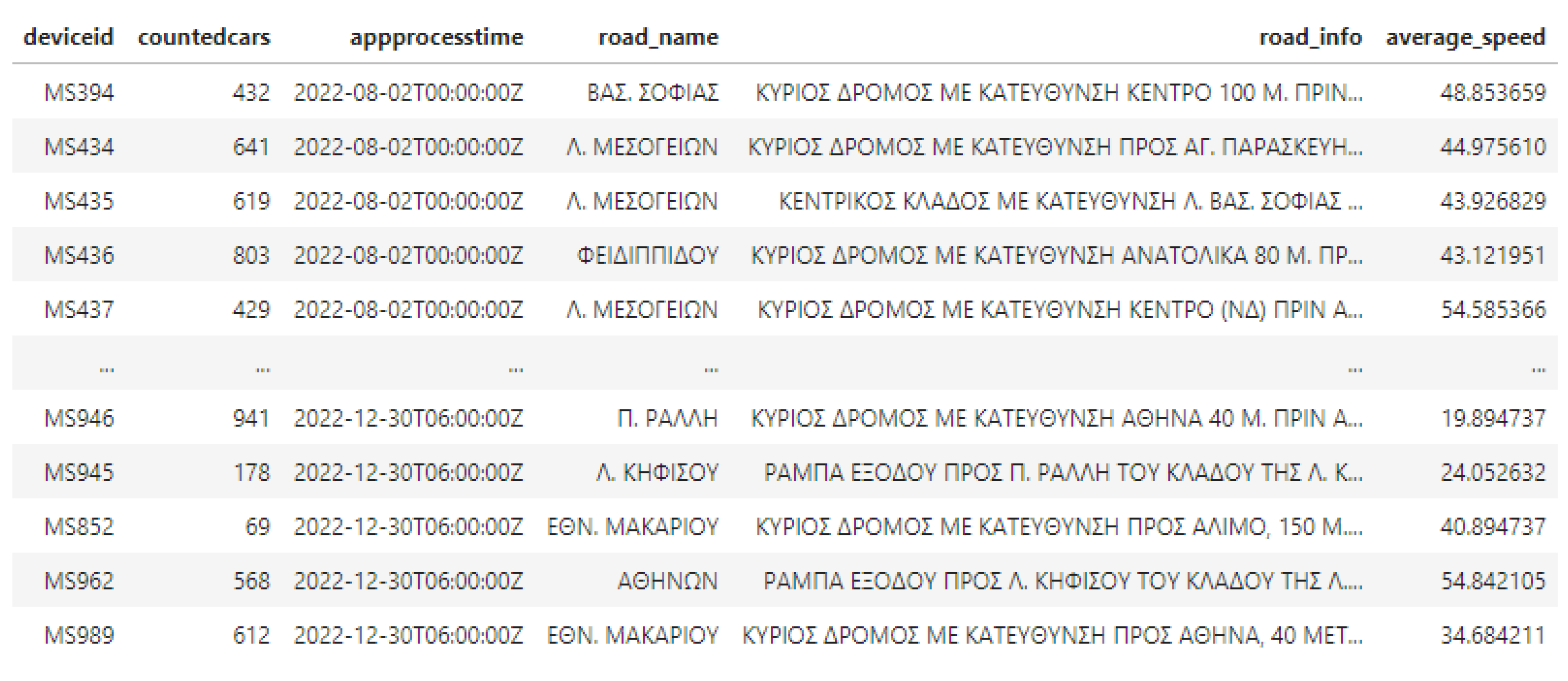
The performance of both the created forecasting models was measured using three metrics, namely Root Mean Squared Error (RMSE), Mean Absolute Error (MAE), and Mean Absolute Percentage Error (MAPE). These metrics are computed as follows:

$$\mathrm{RMSE}=\sqrt{\frac{1}{n}\sum _{i=1}^n{(y_t-\widehat{y_t})}^2}$$

(7)

$$\mathrm{MAE}=\frac{1}{n}\sum _{i=1}^n|y_t-\widehat{y_t}|$$

(8)

$$\mathrm{MAPE}=\frac{1}{n}\sum _{i=1}^n\frac{|y_t-\widehat{y_t}|}{y_t}\ast 100$$

(9)

where $y_t$ denotes the real traffic flow and $\widehat{y_t}$ the corresponding predicted value.

Thereafter, the performance of the models was compared against the performance of two baseline models, i.e., Historical Average (HA) and Autoregressive Integrated Moving Average (ARIMA) that were created using the same dataset.

5. Data Collection

Data.gov.gr is the official Greek data portal for open-government data (OGD). The latest intorsion of the data portal was released in 2020 and provides access to 49 datasets published by the central government, local authorities, or other Greek public bodies classified in ten thematic areas including environment, economy, and transportation.

The major update and innovation of the latest version of the Greek OGD portal was the introduction of an Application Programming Interface (API) that enables accessing and retrieving the data through either a graphical interface or code. The API is freely provided and can be employed to develop various products and services including data intelligence applications. Acquiring a token is needed to use the API by completing a registration process. This process requires providing personal information (i.e., name, email, and organization) as well as the reason for using the API.

The introduction of the API enables the timely provision of dynamic data that are frequently updated. The API can be used, for example, to retrieve datasets describing data related to a variety of transportation systems (e.g., road traffic for the Attica region, ticket validation of Attica’s Urban Rail Transport, and route information and passenger counts of Greek shipping companies). The frequency of data update varies.

The traffic data for the Attica region in Greece were collected from traffic sensors, which periodically transmit traffic information regarding the number of vehicles on specific roads of Attica along with their speed. The data are hourly aggregated to avoid raising privacy issues. Data are updated hourly with only one hour delay.

We used the API provided by data.gov.gr and collected 1,311,608 records for five months, specifically, from 2 August 2022 to 17 December 2022 (138 days). Figure 1 presents a snapshot of the traffic data. Each record includes (a) the unique identifier of the sensor (“deviceid”) (e.g., “MS834”); (b) the road in which the sensor is located along with (“road_name”); (c) a detailed text description of its position (“road_info”); (d) the date and time of the measurement (“appprocesstime”); (e) the absolute number of the vehicles detected by the sensor during the hour of measurement (“countedcars”); and (f) their average speed in km per hour (“average_speed”). The exact position of the sensor is a text description in Greek language and usually provides details including whether the sensor is located on a main or side road, or on an exit or entrance ramp, the direction of the road (e.g., direction to center), and the distance to main roads (e.g., “200 m from Kifisias avenue”).

6. Data Pre-Processing

The traffic data that were retrieved by the Greek open-data portal were produced by 428 sensors. We manually translated the text description of the position of the sensors to latitude and longitude geographic coordinators to be able to present data in a map visualization. Specific position details are missing for one sensor (i.e., the sensor with identifier “MS339”) making it impossible to find its exact coordinates. The sensors are positioned on 93 main roads of the region of Attica.

We then calculated the InterQuartile Range (IQR) of the counted vehicles measured by each sensor to understand the spread of the values. The IQR for each sensor ranges from 0 to 2985.5, while the mean IQR is 826.46. There are eight sensors with IQR equal to 0, which reveals an abnormal behavior since it means that the first and third percentiles are the same and that all the measurements of these sensors are very similar.

Thereafter, we searched for observations that are missing from the traffic data based on two dimensions; (i) the time, where we calculate the missing values per day; and (ii) the sensors, where the missing values per sensor are calculated. Given all the sensor measurements collected and that the traffic data are hourly aggregated, the total number of observations that would have been made by the 428 sensors over the course of the 138 days would be 1,417,536. However, 105,928 observations (or 7.47%) are missing. This number is significantly better than the 20.16% of missing values we discovered in our earlier work that analyzed traffic data collected from data.gov.gr from November of 2020 to June of 2022 [27]. Figure 2 presents the number of missing observations per day for the two different time periods.

We also calculate the percentage of missing observations for each sensor from 2 August 2022 to 17 December 2022. The median percent of missing observations is 33.1% meaning that half of the sensors have less than or equal percentages of missing observations to the median, and half of the sensors have greater than or equal percentages of missing observations to it. The 50% of the sensors have a percentage of missing observations in the range 3–5% (interquartile range box). In addition, according to the whiskers of the boxplot (bottom 25% and top 25% of the data values, excluding outliers), the percentage of missing observations of each sensor may be as low as 3% and as high as 7%. Furthermore, the absolute majority of the sensors (i.e., 85.5%) have less than 10% missing observations. Finally, only five sensors have more than 90% of missing observations and 22 sensors have more than 25% missing values. For the creation of the forecasting models we removed these 22 sensors.

Furthermore, we calculate the number and percentages of anomalies per sensor based on the flow-speed correlation analysis described in Section 3. In order to be able to calculate the number of vehicles that can pass in all lanes, we manually found the number of lanes that each sensor tracks and mapped them to the records. We discovered only 58 records generated by 26 sensors that count more vehicles than the number calculated by the flow-speed correlation analysis. This number is significantly lower compared to the 59.4% of anomalies found in our earlier work. These anomalous measurements relate to only 18 days, which is also a significant improvement related to the analysis of the traffic data from earlier dates when anomalies were generated almost throughout the entire time period. We also calculated the number of anomalies per sensor. This number ranges from 0 to 23 anomalies, while the mean number of detected anomalies per sensor is 0.13 anomalies. In order to create the forecasting model, anomalous observations were removed from the dataset.

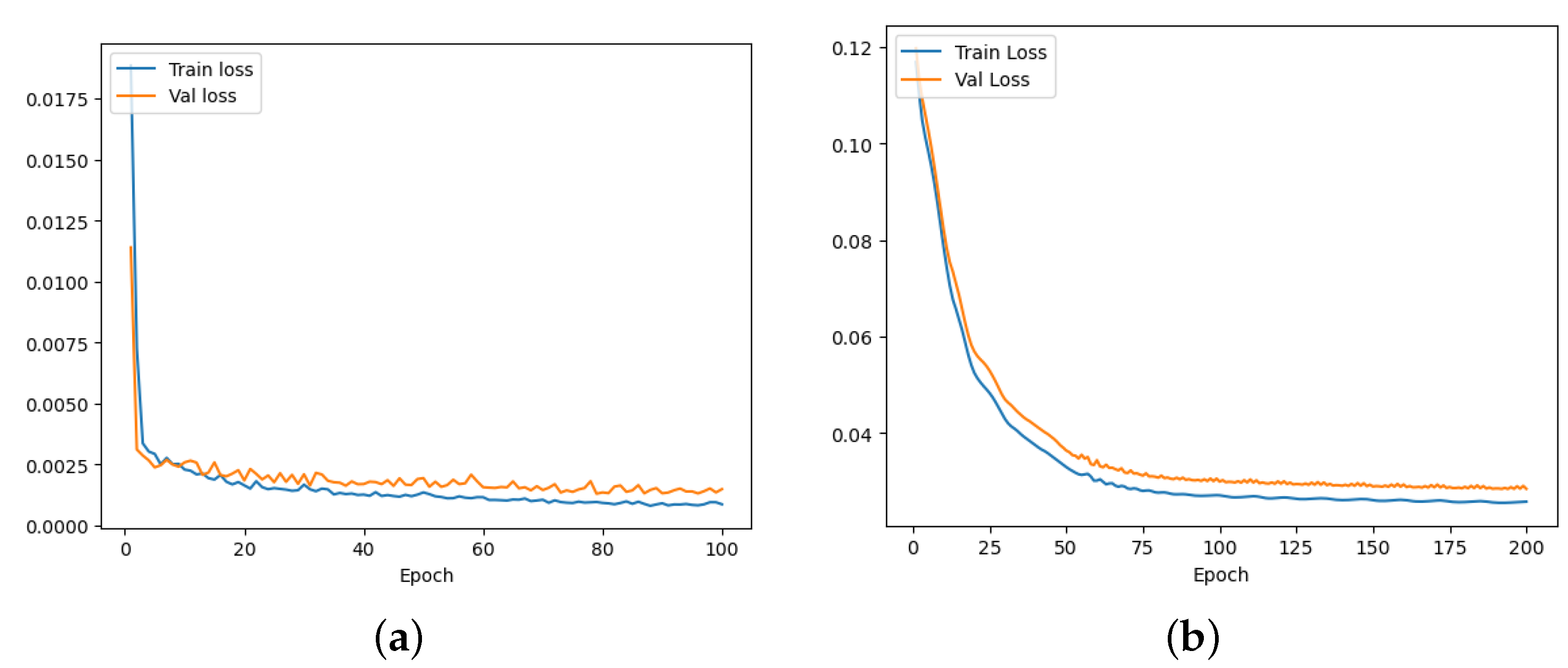
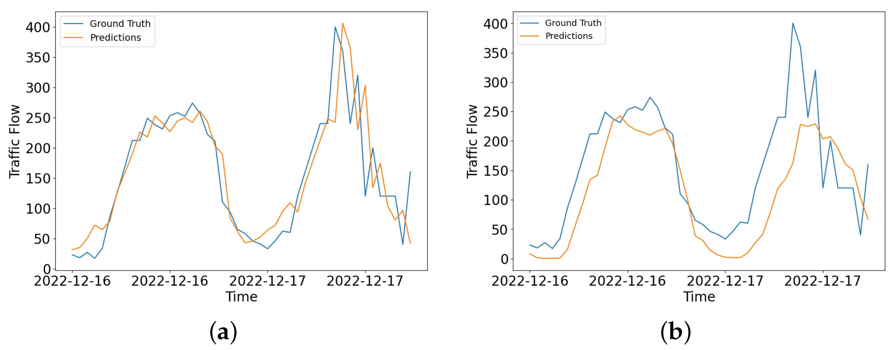
7. Forecasting Traffic Flow

The creation and evaluation of the forecasting GNN models are based on the preprocessed dataset of the previous step. Specifically, 1,354,416 observations generated by 406 sensors were used to create the Temporal Graph Convolutional Network (TGCN) and Diffusion Convolutional Recurrent Neural Network (DCRNN) models and evaluate them against two baseline models, i.e., Historical Average (HA) and Autoregressive Integrated Moving Average (ARIMA).

Table 1. Optimal hyper-parameter values for the two forecasting models.

	TGCN	DCRNN
Learning rate	0.001	0.001
Batch size	50	50
Epochs	100	200
GCN layer sizes (1st/2nd layer)	64/10	-
GRU layer sizes (1st/2nd layer)	256/256	64/64
max steps of random walks	-	3

presents the results of the fine-tuning for both GNN models. More precisely, the learning rate is set to 0.001 for both GNN algorithms as well as a batch size of 50. The training process is deployed using the Adam optimizer for both algorithms. TGCN is trained for 100 epochs and DCRNN for 200 epochs. For the TGCN algorithm the graph convolution layer sizes are set to 64 and 10 units, respectively, while the two GRU layers consist of 256 units. Regarding DCRNN both the encoder and decoder consist of two recurrent layers with 64 units each. Following the paper definition, the maximum steps K of random walks on the graph for the diffusion process is set to 3.

The performance of the GNN-based algorithms is compared with the performance of two baseline methods: Historical Average (HA) and Autoregressive Integrated Moving Average (ARIMA).

Table 2. Performance comparison for GNN and baseline models on the Greek OGD dataset.

Forecasting Horizon	Metric	HA	ARIMA	TGCN	DCRNN
3	RMSE	757.58	534.51	222.2	244.58
	MAE	556.35	466.47	125.12	151.10
	MAPE	7.06%	4.33%	3.98%	6.39%
6	RMSE	757.58	582.33	260.42	331.04
	MAE	556.35	501.13	146.73	212.52
	MAPE	7.06%	7.02%	3.96%	7.664%
9	RMSE	757.58	690.12	267.88	398.31
	MAE	556.35	589.98	156.06	263.54
	MAPE	7.06%	6.98%	4.01%	7.8%

shows the comparison of the performance of different algorithms for three forecasting horizons. All the error metrics are calculated by computing the mean error of each sensor and then averaging it over all 406 sensors. Thus, the evaluation metrics presented in Table 2 represent the overall prediction performance of the proposed algorithms considering the three error metrics among the three forecasting horizons.

Specifically, the two GNN algorithms that emphasize the modeling of spatial dependence perform better in terms of prediction precision compared to the baselines. The results show that the TGCN algorithm outperforms all the other methods regarding all the error metrics for all prediction horizons. For the 3 time steps forecasting horizon, the RMSE error of TGCN and DCRNN is decreased by 58.42% and 54.24% compared with ARIMA model, respectively, and by 70.66% and 67.77% compared with HA. Although the error metrics of all models are increased towards the 6 and 9 time steps horizons, GNN models maintain better prediction results compared with the baselines. To verify which GNN model captures more effectively the spatial–temporal dependencies of traffic flow, we compare the results of TGCN and DCRNN. According to Table 2, the TGCN model demonstrates the best prediction performance among all prediction steps, being able to capture not only short-term, but also long-term spatial–temporal dependencies of the traffic network. This indicates that, for the specific case study, where the traffic flow measurements come from an urban environment where sensors are located close to each other, the graph convolution operation of TGCN captures the complex topology of the sensor network better than the diffusion process of the DCRNN model. Since both models use a similar architecture to model the temporal traffic information with gated recurrent units (GRUs), TGCN effectively captures the spatial dependencies of traffic flows that are obtained from a dense, complex sensor network.

To diagnose the behavior of the proposed models, we created two learning curves (per model) that are calculated based on the metric by which the parameters of the model are optimized, in our case the loss function. To this end, a training learning curve, which is calculated from the loss of the training dataset, and a validation curve, which is calculated from the validation dataset were created. Figure 3 depicts the learning curves of the two GNN models with the number of training epochs in x-axis and scaled MAE in y-axis. TGCN algorithm achieves the lowest validation and training error suggesting superior performance during the training process. Moreover, both validation and training losses regarding the two models, decrease to a point of stability. In addition, Figure 4 and Figure 5 show visualization results of the two GNN algorithms for the 3 h forecasting horizon, for sensors MS109 and MS985, between 16 December 2022 and 17 December 2022. It is observed that TGCN predicts traffic flow slightly better than DCRNN, specifically in high peaks of traffic flow. Therefore, TGCN is more likely to accurately predict abrupt changes in the traffic flow.

8. Discussion

Traffic forecasting is a crucial component of modern intelligent transportation systems, which aim to improve traffic management and public safety [39,70,71]. However, it remains a challenging problem, as several traffic states are influenced by a multitude of complex factors, such as the spatial dependence of intricate urban road networks and complex temporal dynamics. In the literature, many studies have employed graph neural networks (GNNs) which have achieved state-of-the-art performance in traffic forecasting due to their powerful ability to extract spatial information from non-Euclidean structured data commonly encountered in the field of mobility data. The complex spatial dependency of traffic networks can be captured using graph convolutional aggregators on the input graph, while temporal dynamics can be extracted through the integration of recurrent sequential models.

Accessing historical traffic data is essential for deploying models in traffic forecasting. However, obtaining such data can be challenging due to privacy concerns, transmission, and storage restrictions. Most research studies on traffic forecasting using GNNs [19,20,22,56,58,60,62,65,66] have used open traffic data that are already cleansed and preprocessed, including METR-LA, a traffic speed dataset from the highway system of Los Angeles County containing data from 207 sensors during 4 months in 2012 preprocessed by [60], and Performance Measurement System (PeMS) Data (https://pems.dot.ca.gov/(accessed on 3 January 2023)) consisting of several subsets of sensor-generated data across metropolitan areas of California. Although these datasets are often used for benchmarking and comparing the prediction performance of various models, it is important to note that they may not reflect current traffic patterns. This is because traffic data are collected from a past period (e.g., in the case of METR-LA from 2012) and a specific geographical area, such as a highway system, rather than a densely populated urban environment, as typically found in cities.

In recent years, governments and the public sector have started to publish dynamic open-government data (e.g., traffic, environmental, satellite, and meteorological data) freely accessible and reusable on their portals [23,24,25]. This type of data can potentially facilitate the implementation of innovative machine-learning applications [72,73], including state-of-the-art algorithms in traffic forecasting. For instance, the Swiss OGD (https://opentransportdata.swiss/en/ (accessed on 1 November 2022)) portal provides real-time streaming traffic data that is updated every minute. The significance of dynamic open-government data for the deployment of graph neural networks (GNNs) in traffic forecasting cannot be overstated. First, these data sources are open and easily accessible through Application Programming Interfaces (APIs), enabling researchers to retrieve the necessary traffic information without undergoing procedures that include restricted authorization protocols. Furthermore, these data sources are often updated in real time, providing up-to-date traffic information for analysis and prediction. Second, the availability of such data allows for the evaluation and experimentation of relevant GNN models that are currently applied on commonly used benchmarking preprocessed datasets. Therefore, the use of dynamic open-government data has the potential to enhance the accuracy and efficiency of GNN-based traffic-forecasting models.

In this study, two well-known GNN variants, namely Temporal Graph Convolutional Networks (TGCN) and Diffusion Convolutional Recurrent Neural Networks (DCRNN), were used to forecast traffic flow. Specifically, the models were trained on the Greek OGD dataset, and following related literature, 12 past observations, equivalent to 12 past hours, were used to predict traffic flow in the next 3, 6, and 9 h. Before deploying the two models, the OGD traffic dataset underwent pre-processing to address missing observations and anomalies. As a result, sensors with more than 25% missing values and traffic observations detected as anomalies through flow-speed correlation analysis were excluded from the experiments. To model the network topology, a $406\times 406$ adjacency matrix was created based on pairwise distances between traffic sensors.

Both GNN models achieved better prediction performance across all prediction horizons and among all error metrics (RMSE, MAE, MAPE) compared with the two baseline models. Overall, TGCN achieves the best prediction results compared with DCRNN and baselines. For this specific case study, TGCN captures spatial dependencies using graph convolutions from spectral theory, outperforms the DCRNN model that on the other hand, and captures spatial information using bidirectional random walks on the sensor graph with a diffusion process. In summary, both GNN-based models manage to efficiently capture the topological structure of the sensor graph, as well as complex temporal dynamics compared with traditional baselines that only handle time-related features (HA, ARIMA).

The traffic data used to forecast traffic flow in the region of Attica were retrieved by the Greek data portal using the provided API. The data include traffic measurements for the time period 2 August 2022 to 17 December 2022. The exploration of the data showed that the major quality difficulties, including a lot of missing observations as well as anomalous observations, found in the authors’ earlier research [27] have been resolved to a large extent. As a result, these data can be used as a trusted source to make accurate predictions and, thereafter, take informed decisions.

9. Conclusions

The findings of this study demonstrate that open-government data (OGD) is an invaluable resource that can be leveraged by researchers to develop and train more advanced graph neural network (GNN) algorithms. However, the performance of GNNs is highly dependent on the quality and quantity of the data on which they are trained. OGD provides a unique opportunity for researchers to access vast amounts of data from various sources. These data can be used to train GNN models to generalize across a broad range of traffic datasets, resulting in more accurate predictions. Furthermore, the availability of OGD from multiple countries and governments can enable the development of more comprehensive models that can be used to forecast traffic patterns in different regions and under varying conditions. Finally, most studies in the field of traffic forecasting use historical traffic data on small intervals, typically 5 or 15 min. However, this study focuses on the case of the Greek OGD traffic data, which stores traffic data in one-hour intervals. To this end, we plan to conduct further research in dynamic data from other OGD portals that contain datasets of higher quality and smaller aggregated time intervals. In any case, we believe that by continuing to investigate the potential of OGD datasets, will advance the field of traffic forecasting and contribute to the development of more accurate and comprehensive models for predicting traffic patterns.

References

1. Lana, I.; Del Ser, J.; Velez, M.; Vlahogianni, E.I. Road Traffic Forecasting: Recent Advances and New Challenges. IEEE Intell. Transp. Syst. Mag. 2018, 10, 93–109. [Google Scholar] [CrossRef]
2. Varga, N.; Bokor, L.; Takács, A.; Kovács, J.; Virág, L. An architecture proposal for V2X communication-centric traffic light controller systems. In Proceedings of the 2017 15th International Conference on ITS Telecommunications (ITST), Warsaw, Poland, 29–31 May 2017; pp. 1–7. [Google Scholar]
3. Navarro-Espinoza, A.; López-Bonilla, O.R.; García-Guerrero, E.E.; Tlelo-Cuautle, E.; López-Mancilla, D.; Hernández-Mejía, C.; Inzunza-González, E. Traffic Flow Prediction for Smart Traffic Lights Using Machine Learning Algorithms. Technologies 2022, 10, 5. [Google Scholar] [CrossRef]
4. Ran, X.; Shan, Z.; Fang, Y.; Lin, C. An LSTM-Based Method with Attention Mechanism for Travel Time Prediction. Sensors 2019, 19, 861. [Google Scholar] [CrossRef] [PubMed] [Green Version]
5. Ata, A.; Khan, M.A.; Abbas, S.; Khan, M.S.; Ahmad, G. Adaptive IoT empowered smart road traffic congestion control system using supervised machine learning algorithm. Comput. J. 2021, 64, 1672–1679. [Google Scholar] [CrossRef]
6. Kashyap, A.A.; Raviraj, S.; Devarakonda, A.; Shamanth, R.N.K.; Santhosh, K.V.; Bhat, S.J.; Galatioto, F. Traffic flow prediction models—A review of deep learning techniques. Cogent Eng. 2022, 9, 2010510. [Google Scholar] [CrossRef]
7. Zahid, M.; Chen, Y.; Jamal, A.; Mamadou, C.Z. Freeway Short-Term Travel Speed Prediction Based on Data Collection Time-Horizons: A Fast Forest Quantile Regression Approach. Sustainability 2020, 12, 646. [Google Scholar] [CrossRef] [Green Version]
8. Cornago, E.; Dimitropoulos, A.; Oueslati, W. Evaluating the Impact of Urban Road Pricing on the Use of Green Transport Modes. OECD Environ. Work. Pap. 2019. [Google Scholar] [CrossRef]
9. Chin, A.T. Containing air pollution and traffic congestion: Transport policy and the environment in Singapore. Atmos. Environ. 1996, 30, 787–801. [Google Scholar] [CrossRef]
10. Rosenlund, M.; Forastiere, F.; Stafoggia, M.; Porta, D.; Perucci, M.; Ranzi, A.; Nussio, F.; Perucci, C.A. Comparison of regression models with land-use and emissions data to predict the spatial distribution of traffic-related air pollution in Rome. J. Expo. Sci. Environ. Epidemiol. 2008, 18, 192–199. [Google Scholar] [CrossRef] [Green Version]
11. Zhou, Q.; Chen, N.; Lin, S. FASTNN: A Deep Learning Approach for Traffic Flow Prediction Considering Spatiotemporal Features. Sensors 2022, 22, 6921. [Google Scholar] [CrossRef]
12. Kumar, P.B.; Hariharan, K. Time Series Traffic Flow Prediction with Hyper-Parameter Optimized ARIMA Models for Intelligent Transportation System. J. Sci. Ind. Res. 2022, 81, 408–415. [Google Scholar]
13. Yao, H.; Tang, X.; Wei, H.; Zheng, G.; Li, Z. Revisiting Spatial-Temporal Similarity: A Deep Learning Framework for Traffic Prediction. Proc. AAAI Conf. Artif. Intell. 2019, 33, 5668–5675. [Google Scholar] [CrossRef] [Green Version]
14. Yin, X.; Wu, G.; Wei, J.; Shen, Y.; Qi, H.; Yin, B. Deep Learning on Traffic Prediction: Methods, Analysis, and Future Directions. IEEE Trans. Intell. Transp. Syst. 2022, 23, 4927–4943. [Google Scholar] [CrossRef]
15. Qi, Y.; Cheng, Z. Research on Traffic Congestion Forecast Based on Deep Learning. Information 2023, 14, 108. [Google Scholar] [CrossRef]
16. George, S.; Santra, A.K. Traffic Prediction Using Multifaceted Techniques: A Survey. Wirel. Pers. Commun. 2020, 115, 1047–1106. [Google Scholar] [CrossRef]
17. Xie, P.; Li, T.; Liu, J.; Du, S.; Yang, X.; Zhang, J. Urban flow prediction from spatiotemporal data using machine learning: A survey. Inf. Fusion 2020, 59, 1–12. [Google Scholar] [CrossRef]
18. Chen, K.; Chen, F.; Lai, B.; Jin, Z.; Liu, Y.; Li, K.; Wei, L.; Wang, P.; Tang, Y.; Huang, J.; et al. Dynamic Spatio-Temporal Graph-Based CNNs for Traffic Flow Prediction. IEEE Access 2020, 8, 185136–185145. [Google Scholar] [CrossRef]
19. Bui, K.H.N.; Cho, J.; Yi, H. Spatial-temporal graph neural network for traffic forecasting: An overview and open research issues. Appl. Intell. 2022, 52, 2763–2774. [Google Scholar] [CrossRef]
20. Guo, K.; Hu, Y.; Qian, Z.; Sun, Y.; Gao, J.; Yin, B. Dynamic Graph Convolution Network for Traffic Forecasting Based on Latent Network of Laplace Matrix Estimation. Trans. Intell. Transport. Syst. 2022, 23, 1009–1018. [Google Scholar] [CrossRef]
21. Jiang, W.; Luo, J. Graph neural network for traffic forecasting: A survey. Expert Syst. Appl. 2022, 207, 117921. [Google Scholar] [CrossRef]
22. Zhao, L.; Song, Y.; Zhang, C.; Liu, Y.; Wang, P.; Lin, T.; Deng, M.; Li, H. T-GCN: A Temporal Graph Convolutional Network for Traffic Prediction. IEEE Trans. Intell. Transp. Syst. 2020, 21, 3848–3858. [Google Scholar] [CrossRef] [Green Version]
23. Kalampokis, E.; Tambouris, E.; Tarabanis, K. A classification scheme for open government data: Towards linking decentralised data. Int. J. Web Eng. Technol. 2011, 6, 266–285. [Google Scholar] [CrossRef]
24. Kalampokis, E.; Tambouris, E.; Tarabanis, K. Open government data: A stage model. In Proceedings of the Electronic Government: 10th IFIP WG 8.5 International Conference, EGOV 2011, Delft, The Netherlands, 28 August–2 September 2011; Springer: Berlin/Heidelberg, Germany, 2011; pp. 235–246. [Google Scholar]
25. Karamanou, A.; Kalampokis, E.; Tarabanis, K. Integrated statistical indicators from Scottish linked open government data. Data Brief 2023, 46, 108779. [Google Scholar] [CrossRef] [PubMed]
26. Parliament, E. Directive (EU) 2019/1024 of the European Parliament and of the Council of 20 June 2019 on open data and the re-use of public sector information (recast). Off. J. Eur. Union 2019, 172, 56–83. [Google Scholar]
27. Karamanou, A.; Brimos, P.; Kalampokis, E.; Tarabanis, K. Exploring the Quality of Dynamic Open Government Data Using Statistical and Machine Learning Methods. Sensors 2022, 22, 9684. [Google Scholar] [CrossRef] [PubMed]
28. Teh, H.Y.; Kempa-Liehr, A.W.; Wang, K.I.K. Sensor data quality: A systematic review. J. Big Data 2020, 7, 11. [Google Scholar] [CrossRef] [Green Version]
29. Mahrez, Z.; Sabir, E.; Badidi, E.; Saad, W.; Sadik, M. Smart Urban Mobility: When Mobility Systems Meet Smart Data. IEEE Trans. Intell. Transp. Syst. 2022, 23, 6222–6239. [Google Scholar] [CrossRef]
30. Vlahogianni, E.I.; Golias, J.C.; Karlaftis, M.G. Short-term traffic forecasting: Overview of objectives and methods. Transp. Rev. 2004, 24, 533–557. [Google Scholar] [CrossRef]
31. Vlahogianni, E.I.; Karlaftis, M.G.; Golias, J.C. Short-term traffic forecasting: Where we are and where we’re going. Transp. Res. Part C Emerg. Technol. 2014, 43, 3–19. [Google Scholar] [CrossRef]
32. Ermagun, A.; Levinson, D. Spatiotemporal traffic forecasting: Review and proposed directions. Transp. Rev. 2018, 38, 786–814. [Google Scholar] [CrossRef]
33. Williams, B.M.; Hoel, L.A. Modeling and Forecasting Vehicular Traffic Flow as a Seasonal ARIMA Process: Theoretical Basis and Empirical Results. J. Transp. Eng. 2003, 129, 664–672. [Google Scholar] [CrossRef] [Green Version]
34. Yao, Z.; Shao, C.; Gao, Y. Research on methods of short-term traffic forecasting based on support vector regression. J. Beijing Jiaotong Univ. 2006, 30, 19–22. [Google Scholar]
35. Pang, X.; Wang, C.; Huang, G. A Short-Term Traffic Flow Forecasting Method Based on a Three-Layer K-Nearest Neighbor Non-Parametric Regression Algorithm. J. Transp. Technol. 2016, 06, 200–206. [Google Scholar] [CrossRef] [Green Version]
36. Zhang, X.L.; He, G.; Lu, H. Short-term traffic flow forecasting based on K-nearest neighbors non-parametric regression. J. Syst. Eng. 2009, 24, 178–183. [Google Scholar]
37. Sun, S.; Zhang, C.; Yu, G. A bayesian network approach to traffic flow forecasting. IEEE Trans. Intell. Transp. Syst. 2006, 7, 124–132. [Google Scholar] [CrossRef]
38. Jozefowicz, R.; Zaremba, W.; Sutskever, I. An Empirical Exploration of Recurrent Network Architectures. In Proceedings of the 32nd International Conference on Machine Learning, Lille, France, 6–11 July 2015; Volume 37, pp. 2342–2350. [Google Scholar]
39. Ma, X.; Tao, Z.; Wang, Y.; Yu, H.; Wang, Y. Long short-term memory neural network for traffic speed prediction using remote microwave sensor data. Transp. Res. Part C Emerg. Technol. 2015, 54, 187–197. [Google Scholar] [CrossRef]
40. Fu, R.; Zhang, Z.; Li, L. Using LSTM and GRU neural network methods for traffic flow prediction. In Proceedings of the 2016 31st Youth Academic Annual Conference of Chinese Association of Automation (YAC), Wuhan, China, 11–13 November 2016; pp. 324–328. [Google Scholar] [CrossRef]
41. Cui, Z.; Ke, R.; Pu, Z.; Wang, Y. Deep Bidirectional and Unidirectional LSTM Recurrent Neural Network for Network-wide Traffic Speed Prediction. arXiv 2018, arXiv:1801.02143. [Google Scholar]
42. Yu, R.; Li, Y.; Shahabi, C.; Demiryurek, U.; Liu, Y. Deep learning: A generic approach for extreme condition traffic forecasting. In Proceedings of the 2017 SIAM international Conference on Data Mining, Houston, TX, USA, 27–29 April 2017; pp. 777–785. [Google Scholar] [CrossRef] [Green Version]
43. Wu, Y.; Tan, H. Short-term traffic flow forecasting with spatial-temporal correlation in a hybrid deep learning framework. arXiv 2016, arXiv:1612.01022. [Google Scholar]
44. Shi, X.; Chen, Z.; Wang, H.; Yeung, D.Y.; Wong, W.k.; Woo, W.C. Convolutional LSTM Network: A Machine Learning Approach for Precipitation Nowcasting. In Advances in Neural Information Processing Systems; Cortes, C., Lawrence, N., Lee, D., Sugiyama, M., Garnett, R., Eds.; Curran Associates, Inc.: Red Hook, NY, USA, 2015; Volume 28. [Google Scholar]
45. Yu, H.; Wu, Z.; Wang, S.; Wang, Y.; Ma, X. Spatiotemporal Recurrent Convolutional Networks for Traffic Prediction in Transportation Networks. Sensors 2017, 17, 1501. [Google Scholar] [CrossRef] [Green Version]
46. Wu, Z.; Pan, S.; Chen, F.; Long, G.; Zhang, C.; Yu, P.S. A Comprehensive Survey on Graph Neural Networks. IEEE Trans. Neural Netw. Learn. Syst. 2021, 32, 4–24. [Google Scholar] [CrossRef] [Green Version]
47. Girshick, R. Fast R-CNN. In Proceedings of the IEEE International Conference on Computer Vision (ICCV), Santiago, Chile, 7–13 December 2015. [Google Scholar]
48. Li, J.; Chen, X.; Hovy, E.; Jurafsky, D. Visualizing and Understanding Neural Models in NLP. In Proceedings of the 2016 Conference of the North American Chapter of the Association for Computational Linguistics: Human Language Technologies, San Diego, CA, USA, 2–17 June 2016; pp. 681–691. [Google Scholar]
49. Abdel-Hamid, O.; Mohamed, A.R.; Jiang, H.; Deng, L.; Penn, G.; Yu, D. Convolutional Neural Networks for Speech Recognition. IEEE/ACM Trans. Audio Speech Lang. Process. 2014, 22, 1533–1545. [Google Scholar] [CrossRef] [Green Version]
50. Bronstein, M.M.; Bruna, J.; LeCun, Y.; Szlam, A.; Vandergheynst, P. Geometric Deep Learning: Going beyond Euclidean data. IEEE Signal Process. Mag. 2017, 34, 18–42. [Google Scholar] [CrossRef] [Green Version]
51. Qiu, J.; Tang, J.; Ma, H.; Dong, Y.; Wang, K.; Tang, J. DeepInf. In Proceedings of the 24th ACM SIGKDD International Conference on Knowledge Discovery & Data Mining, London, UK, 19–23 August 2018. [Google Scholar] [CrossRef] [Green Version]
52. Henrion, I.; Brehmer, J.; Bruna, J.; Cho, K.; Cranmer, K.; Louppe, G.; Rochette, G. Neural Message Passing for Jet Physics. In Proceedings of the Deep Learning for Physical Sciences Workshop, Long Beach, CA, USA, 4–9 December 2017. [Google Scholar]
53. Duvenaud, D.K.; Maclaurin, D.; Iparraguirre, J.; Bombarell, R.; Hirzel, T.; Aspuru-Guzik, A.; Adams, R.P. Convolutional Networks on Graphs for Learning Molecular Fingerprints. In Advances in Neural Information Processing Systems; Cortes, C., Lawrence, N., Lee, D., Sugiyama, M., Garnett, R., Eds.; Curran Associates, Inc.: Red Hook, NY, USA, 2015; Volume 28. [Google Scholar]
54. Wu, Z.; Pan, S.; Long, G.; Jiang, J.; Zhang, C. Graph wavenet for deep spatial-temporal graph modeling. In Proceedings of the 28th International Joint Conference on Artificial Intelligence, Macao, China, 10–16 August 2019; pp. 1907–1913. [Google Scholar]
55. Agafonov, A. Traffic Flow Prediction Using Graph Convolution Neural Networks. In Proceedings of the 2020 10th International Conference on Information Science and Technology (ICIST), Lecce, Italy, 4–5 June 2020; pp. 91–95. [Google Scholar] [CrossRef]
56. Zhang, Y.; Cheng, T.; Ren, Y.; Xie, K. A novel residual graph convolution deep learning model for short-term network-based traffic forecasting. Int. J. Geogr. Inf. Sci. 2020, 34, 969–995. [Google Scholar] [CrossRef]
57. Veličković, P.; Cucurull, G.; Casanova, A.; Romero, A.; Liò, P.; Bengio, Y. Graph Attention Networks. In Proceedings of the International Conference on Learning Representations, ICLR 2017, Toulon, France, 24–26 April 2017. [Google Scholar]
58. Yu, B.; Yin, H.; Zhu, Z. Spatio-Temporal Graph Convolutional Networks: A Deep Learning Framework for Traffic Forecasting. In Proceedings of the Twenty-Seventh International Joint Conference on Artificial Intelligence. International Joint Conferences on Artificial Intelligence Organization, Stockholm, Sweden, 13–19 July 2018. [Google Scholar] [CrossRef] [Green Version]
59. Atwood, J.; Towsley, D. Diffusion-Convolutional Neural Networks. In Advances in Neural Information Processing Systems; Lee, D., Sugiyama, M., Luxburg, U., Guyon, I., Garnett, R., Eds.; Curran Associates, Inc.: Red Hook, NY, USA, 2015; Volume 29. [Google Scholar]
60. Li, Y.; Yu, R.; Shahabi, C.; Liu, Y. Diffusion Convolutional Recurrent Neural Network: Data-Driven Traffic Forecasting. In Proceedings of the International Conference on Learning Representations, ICLR 2017, Toulon, France, 24–26 April 2017. [Google Scholar]
61. Liang, Y.; Ke, S.; Zhang, J.; Yi, X.; Zheng, Y. GeoMAN: Multi-level Attention Networks for Geo-sensory Time Series Prediction. In Proceedings of the Twenty-Seventh International Joint Conference on Artificial Intelligence, IJCAI-18, Stockholm, Sweden, 13–19 July 2018; pp. 3428–3434. [Google Scholar] [CrossRef] [Green Version]
62. Guo, S.; Lin, Y.; Feng, N.; Song, C.; Wan, H. Attention Based Spatial-Temporal Graph Convolutional Networks for Traffic Flow Forecasting. Proc. AAAI Conf. Artif. Intell. 2019, 33, 922–929. [Google Scholar] [CrossRef] [Green Version]
63. Do, L.N.; Vu, H.L.; Vo, B.Q.; Liu, Z.; Phung, D. An effective spatial-temporal attention based neural network for traffic flow prediction. Transp. Res. Part C Emerg. Technol. 2019, 108, 12–28. [Google Scholar] [CrossRef]
64. Yin, X.; Wu, G.; Wei, J.; Shen, Y.; Qi, H.; Yin, B. Multi-stage attention spatial-temporal graph networks for traffic prediction. Neurocomputing 2021, 428, 42–53. [Google Scholar] [CrossRef]
65. Zheng, C.; Fan, X.; Wang, C.; Qi, J. GMAN: A Graph Multi-Attention Network for Traffic Prediction. Proc. AAAI Conf. Artif. Intell. 2020, 34, 1234–1241. [Google Scholar] [CrossRef]
66. Bai, J.; Zhu, J.; Song, Y.; Zhao, L.; Hou, Z.; Du, R.; Li, H. A3T-GCN: Attention Temporal Graph Convolutional Network for Traffic Forecasting. ISPRS Int. J. Geo-Inf. 2021, 10, 485. [Google Scholar] [CrossRef]
67. Bruna, J.; Zaremba, W.; Szlam, A.; LeCun, Y. Spectral networks and deep locally connected networks on graphs. In Proceedings of the 2nd International Conference on Learning Representations, ICLR 2014, Banff, AB, Canada, 14–16 April 2014. [Google Scholar]
68. Kipf, T.N.; Welling, M. Semi-Supervised Classification with Graph Convolutional Networks. In Proceedings of the International Conference on Learning Representations, ICLR 2017, Toulon, France, 24–26 April 2017. [Google Scholar]
69. Bachechi, C.; Rollo, F.; Po, L. Detection and classification of sensor anomalies for simulating urban traffic scenarios. Clust. Comput. 2022, 25, 2793–2817. [Google Scholar] [CrossRef]
70. Wei, W.; Wu, H.; Ma, H. An autoencoder and LSTM-based traffic flow prediction method. Sensors 2019, 19, 2946. [Google Scholar] [CrossRef] [PubMed] [Green Version]
71. Kuang, L.; Yan, X.; Tan, X.; Li, S.; Yang, X. Predicting taxi demand based on 3D convolutional neural network and multi-task learning. Remote Sens. 2019, 11, 1265. [Google Scholar] [CrossRef] [Green Version]
72. Kalampokis, E.; Karacapilidis, N.; Tsakalidis, D.; Tarabanis, K. Artificial Intelligence and Blockchain Technologies in the Public Sector: A Research Projects Perspective. In Proceedings of the Electronic Government: 21st IFIP WG 8.5 International Conference, EGOV 2022, Linköping, Sweden, 6–8 September 2022; Springer: Berlin/Heidelberg, Germany, 2022; pp. 323–335. [Google Scholar]
73. Karamanou, A.; Kalampokis, E.; Tarabanis, K. Linked open government data to predict and explain house prices: The case of Scottish statistics portal. Big Data Res. 2022, 30, 100355. [Google Scholar] [CrossRef]
Figure 1. A snapshot of the traffic data from data.gov.gr.
Information 14 00228 g001
Figure 2. Number of observations that are missing per day for: (a) 2 August 2022 to 17 December 2022; and (b) 5 November 2020 to 31 June 2022.
Information 14 00228 g002
Figure 3. Learning curves with training and validation error for: (a) Temporal Graph Convolutional networks (TGCN), and (b) Diffusion Convolutional Recurrent Neural Network (DCRNN).
Information 14 00228 g003
Figure 4. Visualizations of prediction results for the forecasting horizon of 3 h for sensor MS109: (a) Temporal Graph Convolutional networks (TGCN), and (b) Diffusion Convolutional Recurrent Neural Network (DCRNN).
Information 14 00228 g004
Figure 5. Visualizations of prediction results for the forecasting horizon of 3 h for sensor MS985: (a) Temporal Graph Convolutional networks (TGCN), and (b) Diffusion Convolutional Recurrent Neural Network (DCRNN).
Information 14 00228 g005