Article

MBTI Personality Prediction Using Machine Learning and SMOTE for Balancing Data Based on Statement Sentences

by
Gregorius Ryan
1,
Pricillia Katarina
1 and
Derwin Suhartono
2,*
1
Computer Science Department, BINUS Graduate Program—Master of Computer Science, Bina Nusantara University, Jakarta 11480, Indonesia
2
Computer Science Department, School of Computer Science, Bina Nusantara University, Jakarta 11480, Indonesia
*
Author to whom correspondence should be addressed.
Information 2023, 14(4), 217; https://doi.org/10.3390/info14040217
Submission received: 21 February 2023 / Revised: 24 March 2023 / Accepted: 28 March 2023 / Published: 3 April 2023

Abstract

:
The rise of social media as a platform for self-expression and self-understanding has led to increased interest in using the Myers–Briggs Type Indicator (MBTI) to explore human personalities. Despite this, there needs to be more research on how other word-embedding techniques, machine learning algorithms, and imbalanced data-handling techniques can improve the results of MBTI personality-type predictions. Our research aimed to investigate the efficacy of these techniques by utilizing the Word2Vec model to obtain a vector representation of words in the corpus data. We implemented several machine learning approaches, including logistic regression, linear support vector classification, stochastic gradient descent, random forest, the extreme gradient boosting classifier, and the cat boosting classifier. In addition, we used the synthetic minority oversampling technique (SMOTE) to address the issue of imbalanced data. The results showed that our approach could achieve a relatively high F1 score (between 0.7383 and 0.8282), depending on the chosen model for predicting and classifying MBTI personality. Furthermore, we found that using SMOTE could improve the selected models’ performance (F1 score between 0.7553 and 0.8337), proving that the machine learning approach integrated with Word2Vec and SMOTE could predict and classify MBTI personality well, thus enhancing the understanding of MBTI.

1. Introduction

The COVID-19 epidemic has altered how people connect and react to one another. Over the past few years, this pandemic has triggered a significant surge in internet and social media usage. According to data from Statista.com, shown in Figure 1, the number of internet users worldwide in 2022 was estimated to reach 5.03 billion people, equivalent to 63.1% of the global population. Meanwhile, the number of social media users worldwide in 2022 was estimated to be around 4.7 billion, or 59% of the global population [1], with the average duration of social media usage in 2022 estimated to be 2 h and 45 min per day. This amount will likely rise over time, with social media users anticipated to reach 5.85 billion by 2027 [2].
Social media platforms such as Facebook, YouTube, WhatsApp, Instagram, WeChat, and TikTok have become the most popular choices for activities in the virtual world [3]. The activities commonly performed on social media vary depending on the user’s interests and personality type. However, these activities include sharing information, communicating with friends, watching videos, creating content, and commenting. With the abundance of activities that can be carried out on social media, understanding someone’s personality is necessary to ensure that the information or content spread on social media (whether created or received) can be tailored to users’ interests and reach the right people.
A personality is a set of traits or characteristics that determine how an individual thinks, feels, and acts. One of the most utilized psychological instruments for understanding and predicting human behavior is the Myers–Briggs Type Indicator (MBTI), a popular instrument for over 50 years that is now widely discussed on social media. Based on Jung’s theory of psychological types (1971) [4], MBTI is a personality measurement model that outlines a person’s preferences along four dimensions, where each distinct dimension describes the propensities of the individual [5]:
  • Introvert (I)–Extrovert (E): This dimension measures how individuals react to their environment, whether they are oriented towards the outside (extrovert) or the inside (introvert).
  • Intuition (N)–Sensing (S): This dimension measures how individuals process information, whether they rely more on information received through direct experience (sensing) or trust their instincts and imagination (intuition) more.
  • Thinking (T)–Feeling (F): This dimension measures how individuals make decisions, whether they rely more on logic and analysis (thinking) or emotions and feelings (feeling).
  • Judgment (J)–Perception (P): This dimension measures how individuals manage their environment, whether they are more inclined to make plans and stick to their tasks (judging) or are more flexible and accepting of change (perceiving).
These four fundamental dimensions can be combined to create one of 16 possible personality types that describe individual personality traits [6]. MBTI has several applications in various fields, including career development, counseling, and relationship improvement [7]. However, like other personality measurement models, MBTI must be used cautiously, not as a diagnostic tool or for making vague generalizations about an individual’s personality. Other personality measurement models include the Big Five Personality Traits, which categorize the human personality into five main domains (openness, conscientiousness, extraversion, agreeableness, and neuroticism) [8], and DISC, which classifies the human personality into four main domains in terms of work and social interactions (dominance, influence, steadiness, and conscientiousness) [9].
Some researchers have argued that the Big Five Personality Traits provide a more comprehensive view of the human personality than MBTI and DISC [10,11]. However, research on MBTI is still relevant and important, as the MBTI model offers a more specific interpretation of an individual’s personality type and can help individuals understand their preferences and how they interact with others [7]. It is also important to note that each model has its strengths and weaknesses, and no model is accurate and covers all aspects of an individual’s personality. This is because each person is unique and different from everyone else. Therefore, it is important to use these models wisely and not view one model as a universal solution to all personality problems.
Research on natural language processing (NLP) for predicting an individual’s MBTI has also been a growing topic in recent years. Using word-embedding technologies and machine learning approaches, NLP techniques can provide computation and extract information from digital communication to identify, predict, and classify individuals into MBTI personality types [12]. However, despite the growing interest in using these techniques for MBTI predictions, some challenges still need to be addressed. Specifically, there is a need for more research on how other word-embedding techniques, machine learning algorithms, and imbalanced data-handling techniques can improve the results and reliability of these predictions.
Word embedding is a computational technique that allows one to convert words or phrases in textual form into numerical vectors to measure how strongly related the given words are [13]. It is used to minimize human communication’s vector dimension and identify features associated with MBTI. Most existing MBTI research used TF-IDF as the weighting technique in information retrieval to assess the relevance of words in a document or corpus [14]. However, in this research, we used Word2Vec as a word-embedding technique to represent words as vectors in a high-dimensional space and capture their relationships with other words in the corpus [15].
In addition to the exploratory use of Word2Vec, this research provides several contributions to the field of MBTI prediction. Firstly, we implemented various machine learning models, including logistic regression (LR), linear support vector classification (LSVC), stochastic gradient descent (SGD), random forest (RF), the extreme gradient boosting classifier (XGBoost), and the cat boosting classifier (CatBoost), which are explained in Section 3.2, to evaluate their effectiveness in predicting MBTI types based on the features identified from the word-embedding method. Secondly, we addressed the imbalanced data issue using SMOTE, which improved the performance of selected models. Finally, we conducted a comprehensive comparison of the performance of each method used, offering insights into the most suitable approach for MBTI prediction based on text data.

2. Related Works

This research was based on previous works classifying MBTI types. Researchers in [7] performed MBTI personality prediction based on data obtained from social media using XGBoost. Before the classification task, the processing started by cleaning and pre-processing the raw data, i.e., through word removal (URLs and stop words) using NLTK, and continued with lemmatization. The following step was vectorizing the processed text by weighting each relevant piece of text using TF-IDF, finishing with the classification task to make a prediction. The results showed that XGBoost achieved an accuracy for I-S of 78.17%, N-S 86.06%, F-T 71.78%, and J-P 65.70%.
In [16], researchers conducted MBTI personality prediction using K-means clustering and gradient boosting. The step before classification consisted of data cleaning and preprocessing (removing URLs and MBTI profile strings, converting all text into lowercase, and lemmatization) and creating vector representations using TF-IDF. The results showed that by using K-means to form the clusters and XGBoost for hyperparameter tuning, the overall accuracy fell in the range of 85–90% for each dimension. Nevertheless, this research had some space for improvement, such as applying more sophisticated parameters; for example, raising the tree depth or increasing the number of iterations on a more balanced dataset could have considerably enhanced the results.
In [17], the researchers performed MBTI personality prediction by comparing different machine learning techniques, namely support vector machine (SVM), the naïve Bayes classifier, and recurrent neural networks, implemented according to the cross-industry standard process for data mining (CRISP-DM), combined with the agile methodology. The results showed that recurrent neural networks (RNNs) with additional bidirectional long short-term memory (BI-LSTM) produced a higher score compared to naïve Bayes and SVM, with an overall accuracy of 49.75%.
The approach proposed in this research was to perform MBTI personality prediction using the word embedding and several machine learning approaches, such as logistic regression (LR), linear support vector classification (LSVC), stochastic gradient descent (SGD), random forest (RF), the extreme gradient boosting classifier (XGBoost), and the cat boosting classifier (CatBoost).

3. Methodology

As shown in Figure 2, several steps had to be carried out to develop the model smoothly, thus achieving the goal of this research. These methods included understanding the dataset with various raw data analysis techniques; preparing the dataset (feature grouping, data cleaning, and data normalization); processing the dataset (tokenization and vectorization); creating and training the model with training data; improving the data (using SMOTE); and evaluating the model through comparisons based on a measurement metric (F1 score).

3.1. Dataset

This section provides an understanding of how the data used in this research were managed and prepared before being used for model training and evaluation.

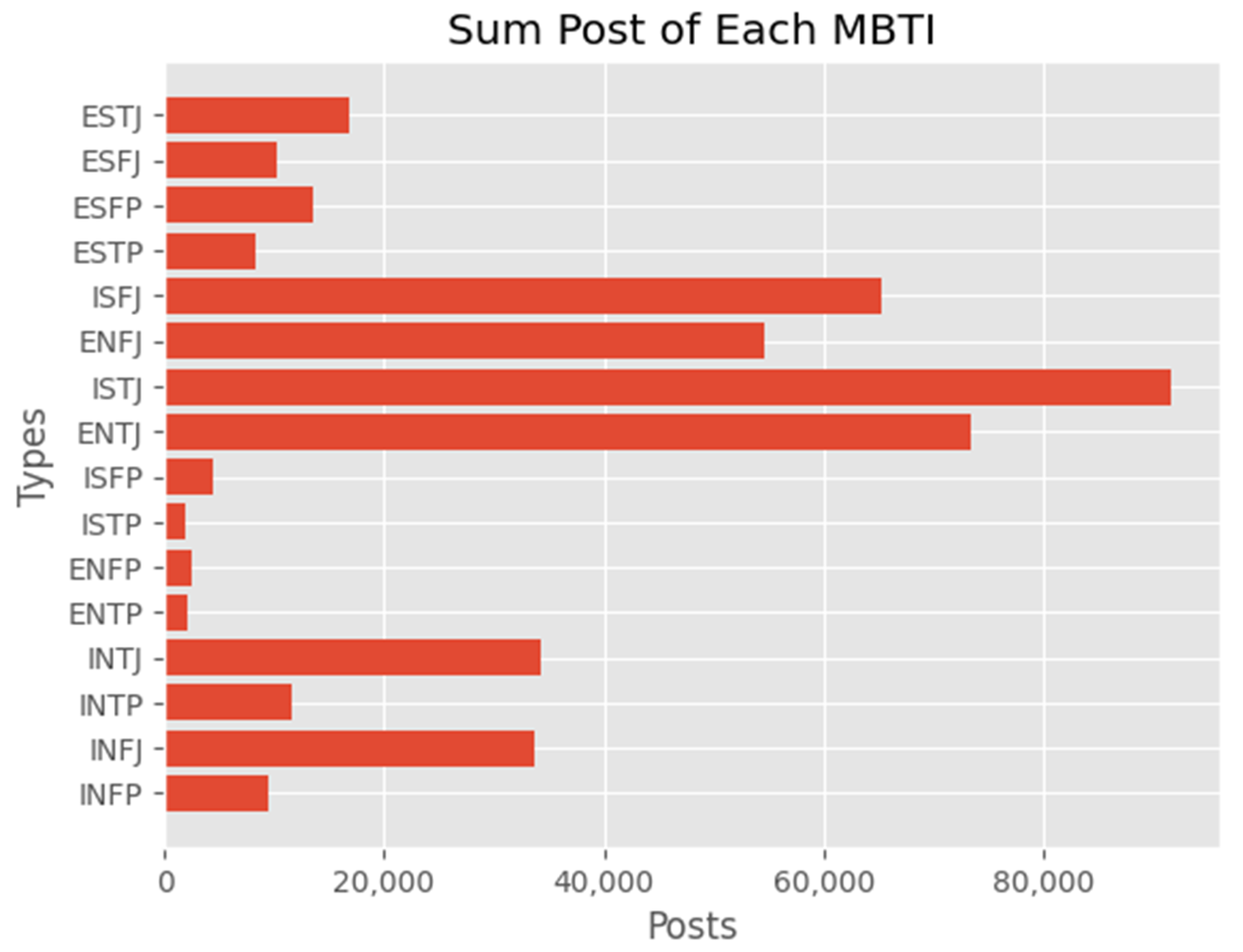
3.1.1. Data Understanding

In this research, the dataset was obtained from the Personality Cafe forum. This dataset is available on Kaggle [18] and comprises 8675 rows, with the first column consisting of MBTI type and the second column containing individuals’ posts (less than or equal to 50 items), divided by “|||” (the 3-pipe symbol). After the symbol was removed, there were 422,845 posts in the entire row of data.
The dataset distribution across the MBTI types presented in Figure 3 showed imbalances for several MBTI types. We considered splitting the classes into 4 instead of 16, conducting a data cleaning process, and performing synthetic minority oversampling techniques (SMOTE) to minimize the imbalanced classes.

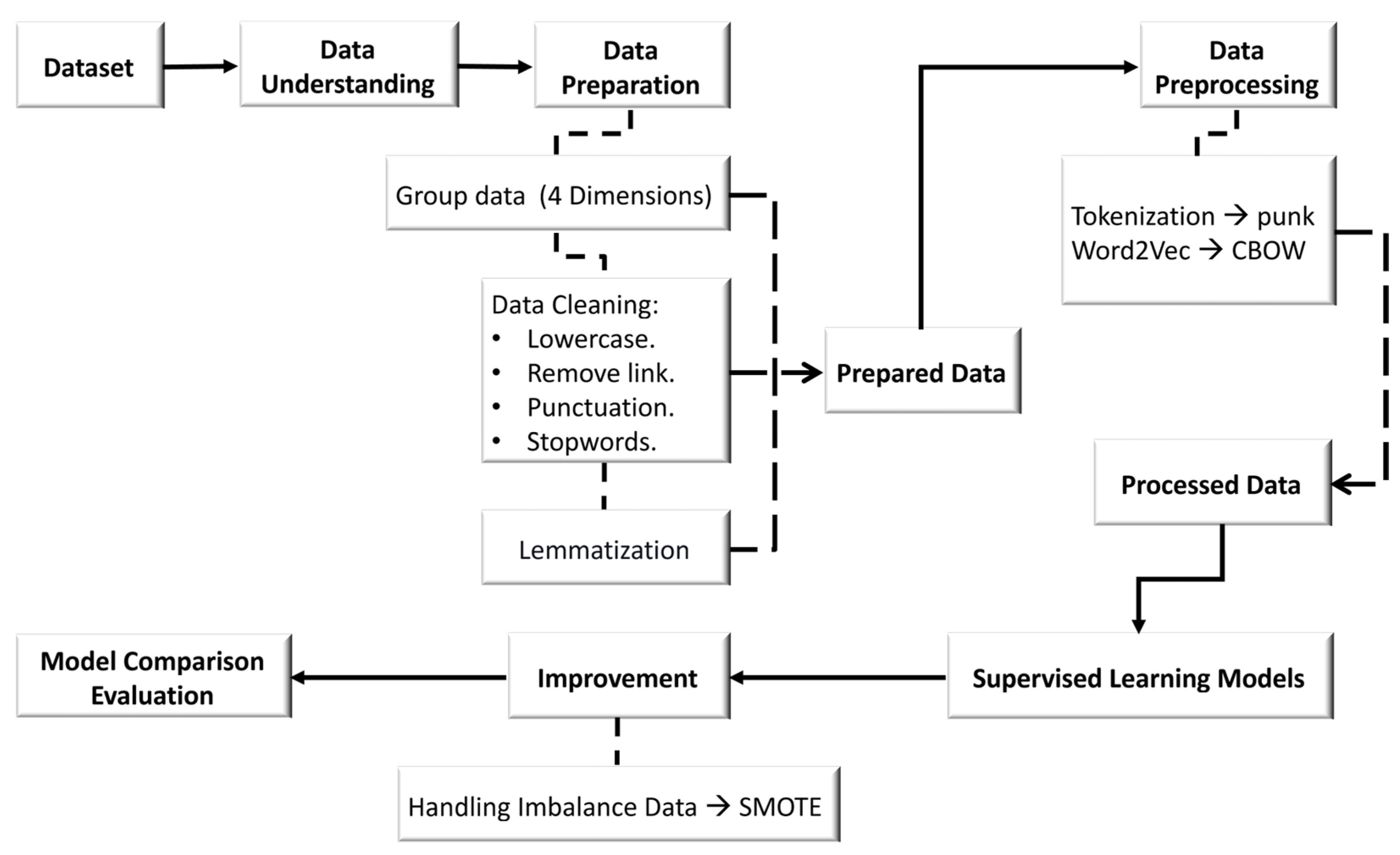
3.1.2. Data Preparation

Four Dimensions

The MBTI type data could be divided into four different classes, namely Introvert (I)–Extrovert (E), Intuition (N)–Sensing (S), Thinking (T)–Feeling (F), and Judgment (J)–Perception (P). Below, we present the distribution of the data for each class.
The distribution of classes presented in Table 1 refers to the main characteristics of each class associated with the indicated MBTI type. This was useful for determining the size of the dataset that was used to classify the MBTI type data.

Data Cleaning

Data cleaning is a crucial step to eliminate unwanted information, improve data quality, and remove noise. It is a process of detecting and correcting or eliminating errors contained in data. Besides improving the data quality, in this research, the implementation of data cleaning also reduced the noise that SMOTE generated. SMOTE can enhance data noise if the original data contain mistakes or inconsistencies, since it creates synthetic data by interpolating between existing datapoints, and any inaccuracies in the original data are transferred to the synthetic data.
Many approaches can be adopted to minimize the noise in imbalanced data; for example, the authors of [19] employed a hybrid framework for fault detection and diagnosis (FDD) frameworks with a signal processing method. This research used data preprocessing and cleaning, one of the three leading solutions proposed in [19], to fix the problem during FDD, which was executed before employing SMOTE to prevent data noise problems. The data-cleaning actions that were implemented for our dataset were as follows:
  • Converting letters to lowercase.
  • Removing links.
  • Removing punctuation.
  • Removing stopwords.
By performing data cleaning, the appropriate data were easier to process. Lemmatization was also performed to transform words in the data into primary forms. The lemmatizer helped us to identify words that were related to each other.

3.1.3. Data Preprocessing

Tokenization

Tokenization was performed to convert textual data (sentences) into tokens (words). Tokenization helped us identify patterns in the data to reduce the number of unidentified words [10]. In this research, tokenization was performed using the ‘punkt’ module from the Natural Language Toolkit (NLTK), which is a collection of computer modules to aid NLP processing supported by Python. The NLTK can be installed from the NLTK website or a package manager such as pip [20]. Then, an English language pattern tokenizer was loaded, and the data in sentence form from the dataset container variable were processed. Afterward, each sentence was cleaned and divided into smaller word units.

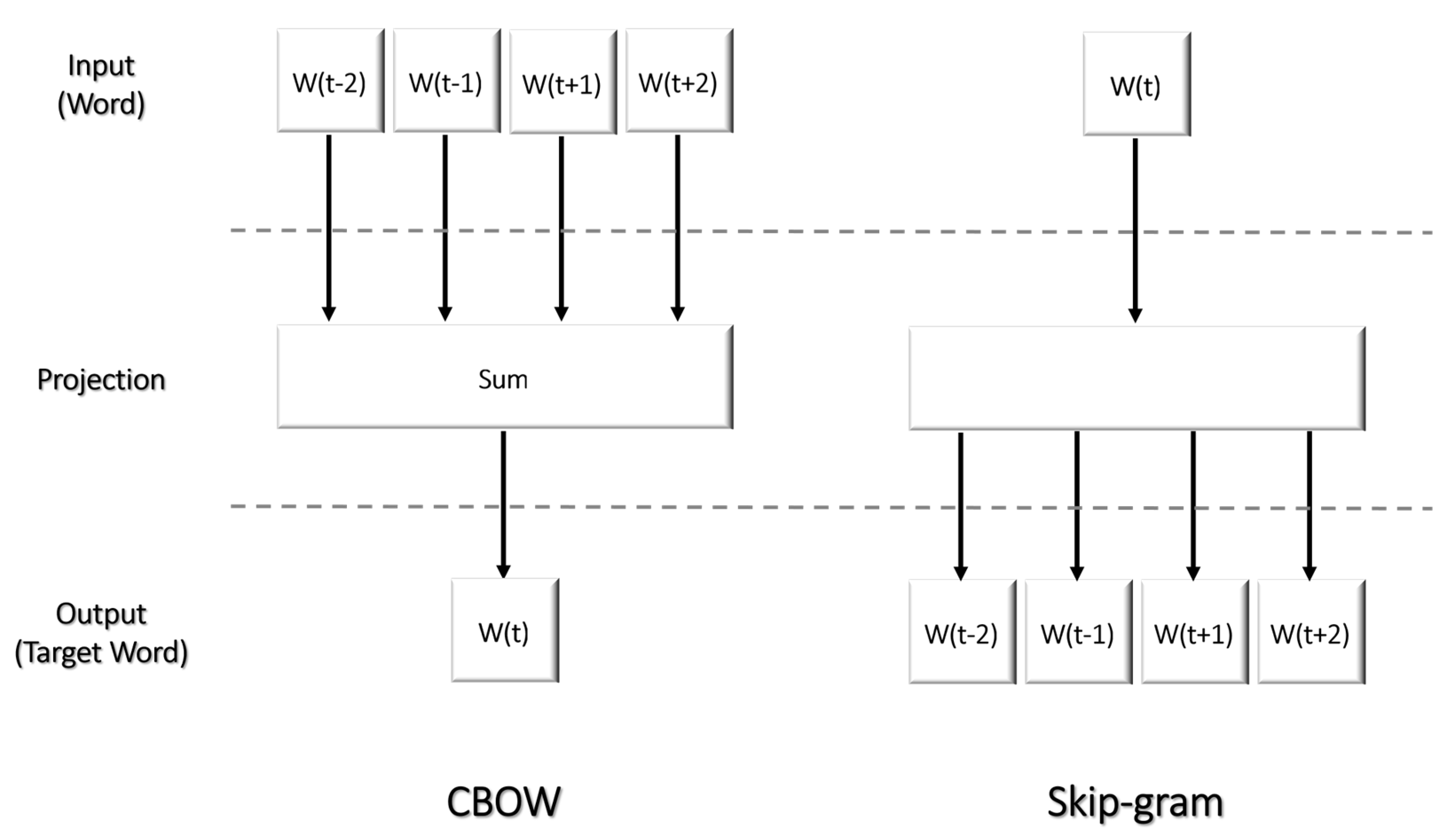
Word Embedding (Word2Vec)

Word embedding helped us measure words that were related to each other. In this research, word embedding was performed using the Word2Vec method. Word2Vec is a text representation technique that learns how to convert words into numerical vectors with a length n. Word2Vec reads sentences and looks for patterns in the word structure. This word-embedding technique provides advantages over the TF-IDF method (a weighting technique in information retrieval and text mining to assess the relevance of words in a document or corpus) [14], as it can learn the relationship between words even if it has never seen that word in training.
Word2Vec consists of two models: Continuous Bag of Words (CBOW) and Skip-gram. Figure 4 shows the architectural differences between the CBOW and Skip-gram models: CBOW predicts a word using the context words in a phrase, while Skip-gram predicts the context words based on the provided word [15]. CBOW is a word-embedding method that involves encoding words into vector form. This method was developed to solve the out-of-vocabulary problem in text corpuses [15]. The equation for CBOW is as follows:
P ( w ) = c C   P ( w | c ) P ( c )
where P ( w ) represents the probability of the word w ; c C   represents the sum of all context words c in the target word’s context window; and P ( w | c )   represents the likelihood of the word w in context c [13].
Skip-gram is also a word-embedding method that involves encoding words into vector form. This method is the opposite of CBOW, as it uses a given word to guess the words around it [15]. The equation for Skip-gram is as follows:
P ( w ) = c C   P ( c | w )   P ( w )
where P ( w )   represents the probability of the word w ; c C represents the sum of all context words c in the target word’s context window; and P ( c | w ) represents the likelihood of the word c that is close to the word w [13].
The process of word embedding using Word2Vec in this research was carried out by initializing the Word2Vec model using the gensim Python library with sentence, size, window, and min_count parameters. The sentence parameter was a set of sentences to be used to train the model, the size parameter set the vector size for each word, the window parameter specified the number of words to the left and right of the word to be examined, and the min_count parameter specified the minimum number of words required in the phrase.
We chose the CBOW model over the Skip-gram model since CBOW could better represent frequent words and be trained quicker than Skip-gram [15]. After initialization was completed, the Word2Vec model was trained with 50 epochs and total_examples parameters. The epoch parameter determined how many times the model iterated through the training data, while the total_examples parameter set the total number of sentences to be processed. Afterwards, the model was used to generate a vector of a sentence with values from the pre-defined Word2Vec model, and a high-dimensional matrix could be created.

Splitting of Data into Training Set and Testing Set

In this research, we split the data using the train_test_split() function in Python (available in the sklearn.model_selection module of the scikit-learn library [21]) with a ratio of 70% for training and 30% for the testing set. The training set was used to train the classification model, and the testing set was used to test the model that had been constructed. After performing all these steps, we were ready to perform the MBTI classification.

3.2. Modeling

This section provides a general overview of the six machine learning models that were used in the research. For each model, we briefly explain the basic concepts and how it works, as well as providing some additional information.

3.2.1. Logistic Regression

Logistic regression (LR) is a statistical approach that examines the relationships between multiple independent variables and a categorical dependent variable. This model predicts the probability of an event occurring based on a logistic curve fitted to the data [22]. There are two types of LR models: binary logistic regression and multinomial logistic regression. This research used binary logistic regression to predict the dimension types for four dimensions. Using binary logistic regression, the model learned a set of coefficients for each feature that indicated that feature’s contribution to the likelihood that the target variable was positive [23]. Following this, the anticipated probabilities were thresholded to provide binary class predictions in each dimension. The equation for binary logistic regression is as follows:
log ( p 1 p ) = b 0 + b 1 X 1 + + b n X n
where p represents the probability of dependent variable = 1 ;   b 0 is an intercept; and b 1 ,   ,   b n are the coefficients linked with independent variables X 1 ,   ,   X n [24]. The equation consists of the sigmoid function mapping of any real number between 0 and 1. The logistic regression model’s coefficients are determined using maximum likelihood estimation, which includes determining the coefficient values that maximize the probability of the observed data given the model [25].

3.2.2. Linear Support Vector Classification

Linear support vector classification (LSVC) is a popular supervised learning model for text classification based on the concept of support vector machine (SVM). It was introduced by Vladimir Vapnik and Corinna Cortes to handle two-group classification problems [26]. SVM operates by finding the optimal boundary in the vector space that separates the two classes [27], transforming the data domain into a response set and splitting it by drawing a hyperplane [28]. The optimization issue solved by the SVM necessitates locating the hyperplane that provides the greatest partition between classes while simultaneously presenting the most significant space between the closest examples of each class (known as support vectors) [29]. The equation for LSVC is as follows:
y = w T x + b
where y is the predicted class, w T is the weight, x is the featuring vector, and b is the bias [26]. The prediction result is based on the sign produced by the equation, where positive values correspond to one class and negative values to another class.

3.2.3. Stochastic Gradient Descent

Stochastic gradient descent (SGD) is a supervised learning model for optimizing linear classifiers and regressors based on convex loss functions, such as support vector machines and logistic regression [30]. SGD is a modified version of the gradient descent (GD) algorithm focusing on random probability (stochastic) [31]. The model iteratively adjusts the parameters of a function to find its minimum or maximum, improving the accuracy of predictions [32]. SGD uses several hyperparameters to optimize its performance on analyzed data. These hyperparameters can be adjusted to fine-tune the model’s performance [31]. The equation for SGD is as follows:
w t + 1 = w t γ t   w Q ( z t ,   w t )
where w t is the weighted vector; γ t is the learning rate; and w   Q ( z t ,   w t ) is the gradient of the loss function with respect to weight [32].

3.2.4. Random Forest

Random forest (RF) is a supervised learning model introduced by Breiman that consists of multiple decision trees. The trees in the ensemble are created by selecting a random sample of training data with replacements [33]. RF combines the predictions of multiple randomized decision trees and takes the average to make a final prediction, resulting in a more accurate prediction [34]. Because of its simplicity, accuracy, and adaptability, it is one of the most popular and commonly used machine learning algorithms [35]. The equation for RF is as follows:
Z = arg m a x 1 T t = 1 T P t ( y x )
where P t ( y x ) represents the probability distribution of a specific tree, and x is a collection of test samples [36]. Using random forest for prediction modeling has the advantage of being able to handle large datasets with numerous predictor variables. However, in practical applications, it is often necessary to reduce the number of predictors used for making outcome predictions to improve the efficiency of the process [37].

3.2.5. Extreme Gradient Boosting

Extreme gradient boosting (XGBoost) is an implementation of the gradient boosting decision tree (GBDT) developed by Friedman in 2001 [38]. The XGBoost package consists of an effective linear model solver and a tree-learning algorithm. It facilitates object processes such as regression, ranking, and classification. The formula used in XGBoost is the objective function formula. This objective function determines how the model makes predictions and minimizes the error between the predictions and the actual target. The objective function equation in XGBoost is:
L ( t ) = i = 1 n l ( y i ,   y ^ i ( t 1 ) + f t ( x i ) ) + Ω ( f t )
where L is the loss function that determines how big the error is between the actual target y i and the prediction y ^ i , and Ω is the regularization term that restricts the model from overfitting. Because XGBoost is created using multiple cores [39], and several hyperparameters can be optimized, XGBoost can improve the model’s performance and speed by minimizing overfitting, enhancing generalization performance, and shortening the computation time, making it a popular algorithm in machine learning [40].

3.2.6. CatBoost

CatBoost is a gradient boosting decision tree (GDBT) model developed by Yandex. It includes two significant algorithmic advancements compared to traditional GBDT:
  • It utilizes a permutation-driven ordered boosting method instead of the conventional approach.
  • It employs a unique categorical feature-processing algorithm.
These improvements were designed to address a specific type of target leakage in previous GBDT implementations, which could lead to inaccurate predictions [41,42].
The CatBoost equation cannot be expressed with a single formula as it is a complex machine learning algorithm. This algorithm combines several techniques, such as gradient boosting, decision trees, and categorical feature handling. The algorithm builds small trees iteratively using gradient boosting techniques to improve the model’s accuracy by minimize the expected loss [42], as shown in Equation (8) below:
h t = arg m i n   E   ( δ L y δ F t 1 h ) 2 arg m i n 1 n ( δ L y δ F t 1 h ) 2 h H
It is also designed to handle categorical features in a better way compared to other gradient boosting algorithms by utilizing modified target-based statistics that help to reduce the computational burden of processing categorical features [43]. CatBoost uses categorical encoding techniques such as one-hot encoding, target statistics encoding, and binning for categorical feature handling. This allows the algorithm to process categorical features and improve prediction accuracy efficiently [44]. Below is the equation to estimate the i t h categorical variable with the k - t h element:
x ^ k i = x j D k 𝟙 { x j i = x k i }   ·   y j + a   p x j D k 𝟙 { x j i = x k i } + a
where parameter a must be greater than zero, and a frequently used value for p (prior) is the average target value in the training dataset D . A comprehensive explanation of the CatBoost algorithm can be obtained from [42].

3.3. Data Balancing Using SMOTE and F1 Score Metric

This section provides a general explanation of using SMOTE to address data imbalance problems and using the F1 score as the evaluation metric in this research.

3.3.1. SMOTE

The synthetic minority oversampling technique (SMOTE) is an approach that uses “synthetic” instances to oversample the minority class to resolve unbalanced data. Using synthetic examples in “feature space” rather than “data space” means that SMOTE is conducted based on the value and characteristics of the data relationships instead of focusing on all datapoints. SMOTE works by injecting synthetic cases along the lines connecting any or all of the k-nearest neighbors of each minority class and oversampling each minority class. Neighbors from the k-nearest neighbors are picked randomly based on the amount of oversampling needed [45].

3.3.2. F1 Score

The F1 score is a metric used to evaluate a classifier’s performance by combining its precision and recall. It combines these two measures into a single statistic by taking the harmonic mean of the precision and recall values [46]. The F1 score is commonly used to compare the effectiveness of different classifiers.
F 1 = 2 P R P + R
where P is precision, and R is recall.

4. Result and Discussion

In this research, the classification process involved several machine learning approaches that were described in Section 3.2. The results are represented in Table 2, showing that the MBTI personality classification process was divided into four different dimensions, and various results were obtained. The best model for predicting MBTI personality type was logistic regression (LR), with an average F1 score of 0.8282 and the highest score of 0.8818 obtained for dimension 3 (N/S); followed by LSVC, with average score 0.8266, SGD, with average score 0.8070; Catboost, with average score 0.7952; XGBoost, with average score 0.7804; and RF, with average score 0.7383. The F1 score can be interpreted as a harmonic average of precision and recall, where the best score is 1 and the worst is 0 [47]. Because the LR value was close to 1, the LR model could capture patterns in the data and identify various types of personality more accurately than the other models.
Furthermore, we improved the results for each model using SMOTE, a technique to handle the imbalance of MBTI data in this research. SMOTE increased the number of datapoints by generating new samples from existing ones. This technique helped to make the dataset more balanced, which improved the model’s performance, as seen clearly from the results in Table 3.
Table 4 shows that the LR model experienced an improvement from the previous score of 0.8282 to a score of 0.8337, with dimension 3 (N/S) again obtaining the highest score at 0.8821. Furthermore, the results showed an increase in the scores for some dimensions and a decrease in the scores for others with specific models. Overall, the results showed that the LR model was better-suited for MBTI personality prediction using word embedding and machine learning than the other models. The use of SMOTE also improved the results significantly, further validating this technique’s effectiveness.
Based on the results of this research, we realized that many different methods and dimensions could be used to assess the efficacy of a machine learning model for predicting MBTI personality type. Previous research used either 4 dimensions or 16 dimensions, as well as combining machine learning with deep learning to obtain the optimum results or using machine learning alone, as in this research.
Research conducted by Amirhosseini and Hassan [7] used the XGBoost method, and then divided the data into four dimensions and yielded an average accuracy of 0.7543. Mushtaq et al. [16] used the K-means clustering and XGBoost methods and divided the data into four dimensions, yielding an average accuracy of 0.8630. Moreover, Ontoum and Jonathan [17] used recurrent neural networks with BI-LSTM and divided the data into 16 dimensions, yielding an average accuracy of 0.4975. According to these varied results, the research conducted by Mushtaq et al. [16] yielded the highest values, though the process and performance metrics differed. Our research process for predicting MBTI used Word2Vec as a word-embedding technique and SMOTE as a technique to handle the imbalanced data. Moreover, the metric we used was the F1 score, whereas the previous research used accuracy as the primary metric. We chose the F1 score as the primary metric rather than accuracy since, in this case, we were dealing with an imbalanced dataset, and the F1 score considers both precision and recall, offering a more accurate estimate of a model’s ability to accurately identify both positive and negative classes [46].
In sum, the LR model, with an F1 score of 0.8337 after the implementation of SMOTE, along with the various data-handling techniques proposed in this research, could help other researchers identify problems that might have been overlooked in previous or subsequent research regarding personality predicting.

5. Conclusions

In this research, the prediction of MBTI personality types based on sentences was performed using the Python programming language. The proposed method used in this research involved Word2Vec embedding, SMOTE, and six machine learning classifiers that we trained and tested individually to predict MBTI personality type. The results showed that the best machine learning model for predicting MBTI type dimensions in this research was logistic regression (LR), with an average F1 score of 0.8282. The employed SMOTE technique also showed a better result, with the F1 score increasing to 0.8337, and dimension 3 (N/S) had the highest score of 0.8821. The acceptable threshold for the F1 score varies depending on the application, but an F1 score close to 1 is generally considered high for data classification. Therefore, this result was more favorable when compared to the other models considered, showing that the proposed approach could be used to enhance our understanding of MBTI and could be employed in various applications that require personality classification.
In future works, we plan to enhance our research by incorporating other data sources using more advanced machine learning algorithms and deep learning architectures, such as convolutional neural networks (CNNs) [48] and recurrent neural networks (RNNs) [49], to predict MBTI personality types more accurately. Furthermore, we plan to experiment with different word-embedding techniques, such as global vectors for word representation (GloVe) [50] and bidirectional encoder representations from transformers (BERT) [51], to more accurately represent the semantic relationships between words. On top of this, we aim to include information from other sources, such as social media data, to enrich our understanding of personality types. Finally, we believe that we can achieve even more accurate results by incorporating recent advancements in natural language processing techniques such as transformers. With these future research directions, we aim to achieve an even better F1 score and provide a more comprehensive analysis of the MBTI personality types.

Author Contributions

Conceptualization, G.R. and P.K.; methodology, G.R. and P.K.; software, G.R. and P.K.; validation, G.R. and P.K.; formal analysis, G.R. and P.K.; investigation, G.R. and P.K.; resources, G.R. and P.K.; data curation, G.R. and P.K.; writing—original draft preparation, G.R. and P.K.; writing—review and editing, G.R., P.K. and D.S.; visualization, G.R. and P.K.; supervision, D.S.; project administration, D.S.; funding acquisition, D.S. All authors have read and agreed to the published version of the manuscript.

Funding

This research received no external funding.

Institutional Review Board Statement

Not applicable.

Informed Consent Statement

Not applicable.

Data Availability Statement

The (MBTI) Myers–Briggs Personality Type Dataset is available from Kaggle at https://www.kaggle.com/datasets/datasnaek/mbti-type (accessed on 20 November 2022).

Acknowledgments

The work was supported by Bina Nusantara University. The authors are also profoundly grateful for the reviewers’ helpful comments and suggestions, which helped improve the presentation.

Conflicts of Interest

The authors declare no conflict of interest.

Abbreviations

The following abbreviations are used in this manuscript:
BERTBidirectional encoder representations from transformers
BI-LSTMBidirectional long short-term memory
CatBoostCat boosting classifier
CBOWContinuous bag of words
CNNConvolutional neural network
CRISP-DMCross-industry standard process for data mining
DimDimension
DISCDominance, influence, steadiness, and conscientiousness
EExtrovert
FFeeling
FDDFault detection and diagnosis
GDBTGradient boosting decision tree model
GloVeGlobal vectors for word representation
IIntrovert
JJudgment
LRLogistic regression
LSVCLinear support vector classification
MBTIMyers–briggs type indicator
NIntuition
NLPNatural language processing
NLTKNatural language toolkit
OCEANOpenness, conscientiousness, extraversion, agreeableness, and neuroticism
PPerception
RFRandom forest
RNNRecurrent neural network
SSensing
SGDStochastic gradient descent
SMOTESynthetic minority oversampling technique
SVMSupport vector machine
TThinking
TF-IDFTerm frequency-inverse document frequency
XGBoostExtreme gradient boosting classifier

References

  1. Petrosyan, A. Worldwide Digital Population July 2022. Statista. Available online: https://www.statista.com/statistics/617136/digital-population-worldwide/ (accessed on 6 January 2023).
  2. Dixon, S. Number of Social Media Users Worldwide 2017–2027. Statista. 2022. Available online: https://www.statista.com/statistics/278414/number-of-worldwide-social-network-users/ (accessed on 6 January 2023).
  3. Dixon, S. Global Social Networks Ranked by Number of Users 2022. Statista. 2022. Available online: https://www.statista.com/statistics/272014/global-social-networks-ranked-by-number-of-users/ (accessed on 6 January 2023).
  4. Myers, I.B.; Mccaulley, M.H. Manual, a Guide to the Development and Use of the Myers-Briggs Type Indicator; Consulting Psychologists Press: Palo Alto, CA, USA, 1992. [Google Scholar]
  5. The Myers & Briggs Foundation—MBTI® Basics. Available online: https://www.myersbriggs.org/my-mbti-personality-type/mbti-basics/home.htm (accessed on 8 January 2023).
  6. Varvel, T.; Adams, S.G. A Study of the Effect of the Myers Briggs Type Indicator. In Proceedings of the 2003 Annual Conference Proceedings, Nashville, TN, USA, 22–25 June 2003. [Google Scholar] [CrossRef]
  7. Amirhosseini, M.H.; Kazemian, H. Machine Learning Approach to Personality Type Prediction Based on the Myers–Briggs Type Indicator®. Multimodal Technol. Interact. 2020, 4, 9. [Google Scholar] [CrossRef] [Green Version]
  8. Ong, V.; Rahmanto, A.D.; Suhartono, D.; Nugroho, A.E.; Andangsari, E.W.; Suprayogi, M.N. Personality Prediction Based on Twitter Information in Bahasa Indonesia. In Proceedings of the 2017 Federated Conference on Computer Science and Information Systems, Prague, Czech Republic, 3–6 September 2017. [Google Scholar] [CrossRef] [Green Version]
  9. DISC Profile. What Is DiSC®. Discprofile.com. 2021. Available online: https://www.discprofile.com/what-is-dis (accessed on 9 January 2023).
  10. John, O.P.; Srivastava, S. The Big-Five Trait Taxonomy: History, Measurement, and Theoretical Perspectives; University of California: Berkeley, CA, USA, 1999; pp. 102–138. [Google Scholar]
  11. Tandera, T.; Suhartono, D.; Wongso, R.; Prasetio, Y.L. Personality Prediction System from Facebook Users. Procedia Comput. Sci. 2017, 116, 604–611. [Google Scholar] [CrossRef]
  12. Santos, V.G.D.; Paraboni, I. Myers-Briggs Personality Classification from Social Media Text Using Pre-Trained Language Models. JUCS—J. Univers. Comput. Sci. 2022, 28, 378–395. [Google Scholar] [CrossRef]
  13. Mikolov, T.; Sutskever, I.; Chen, K.; Corrado, G.S.; Dean, J. Distributed Representations of Words and Phrases and Their Compositionality. arXiv 2013, arXiv:1310.4546. [Google Scholar] [CrossRef]
  14. Aizawa, A. An Information-Theoretic Perspective of Tf–Idf Measures. Inf. Process. Manag. 2003, 39, 45–65. [Google Scholar] [CrossRef]
  15. Mikolov, T.; Chen, K.; Corrado, G.; Dean, J. Efficient Estimation of Word Representations in Vector Space. arXiv 2013, arXiv:1301.3781. [Google Scholar] [CrossRef]
  16. Mushtaq, Z.; Ashraf, S.; Sabahat, N. Predicting MBTI Personality Type with K-Means Clustering and Gradient Boosting. In Proceedings of the 2020 IEEE 23rd International Multitopic Conference (INMIC), Bahawalpur, Pakistan, 5–7 November 2020. [Google Scholar] [CrossRef]
  17. Ontoum, S.; Chan, J.H. Personality Type Based on Myers-Briggs Type Indicator with Text Posting Style by Using Traditional and Deep Learning. arXiv 2022, arXiv:2201.08717. [Google Scholar] [CrossRef]
  18. (MBTI) Myers-Briggs Personality Type Dataset. Available online: https://www.kaggle.com/datasets/datasnaek/mbti-type (accessed on 20 November 2022).
  19. Jalayer, M.; Kaboli, A.; Orsenigo, C.; Vercellis, C. Fault Detection and Diagnosis with Imbalanced and Noisy Data: A Hybrid Framework for Rotating Machinery. Machines 2022, 10, 237. [Google Scholar] [CrossRef]
  20. Loper, E.; Steven, B. NLTK: The Natural Language Toolkit. arXiv 2019, arXiv:cs/0205028. [Google Scholar] [CrossRef]
  21. Sklearn.model_selection.train_test_split–Scikit-Learn 0.20.3 Documentation. 2018. Available online: https://scikit-learn.org/stable/modules/generated/sklearn.model_selection.train_test_split.html (accessed on 10 January 2023).
  22. Nick, T.G.; Campbell, K.M. Logistic Regression. In Topics in Biostatistics; Springer: Berlin/Heidelberg, Germany, 2007; pp. 273–301. [Google Scholar] [CrossRef]
  23. Hastie, T.; Tibshirani, R.; Friedman, J.H.; Friedman, J.H. The Elements of Statistical Learning: Data Mining, Inference, and Prediction; Springer: New York, NY, USA, 2001. [Google Scholar]
  24. Binary Logistic Regression—A Tutorial. 2021. Available online: https://digitaschools.com/binary-logistic-regression-introduction/ (accessed on 10 January 2023).
  25. Wong, G.Y.; Mason, W.M. The Hierarchical Logistic Regression Model for Multilevel Analysis. J. Am. Stat. Assoc. 1985, 80, 513–524. [Google Scholar] [CrossRef]
  26. Cortes, C.; Vapnik, V. Support-Vector Networks. Mach. Learn. 1995, 20, 273–297. [Google Scholar] [CrossRef]
  27. Zhang, W.; Yoshida, T.; Tang, X. Text Classification Based on Multi-Word with Support Vector Machine. Knowl. Based Syst. 2008, 21, 879–886. [Google Scholar] [CrossRef]
  28. Suthaharan, S. Support Vector Machine. Mach. Learn. Model. Algorithms Big Data Classif. 2016, 36, 207–235. [Google Scholar] [CrossRef]
  29. Platt, J. Sequential Minimal Optimization: A Fast Algorithm for Training Support Vector Machines; Microsoft: Washington, DC, USA, 1998. [Google Scholar]
  30. Stochastic Gradient Descent—Scikit-Learn 0.23.2 Documentation. Available online: https://scikit-learn.org/stable/modules/sgd.html (accessed on 11 January 2023).
  31. Gaye, B.; Zhang, D.; Wulamu, A. Sentiment Classification for Employees Reviews Using Regression Vector- Stochastic Gradient Descent Classifier (RV-SGDC). PeerJ Comput. Sci. 2021, 7, e712. [Google Scholar] [CrossRef]
  32. Bottou, L. Stochastic Gradient Descent Tricks. In Neural Networks: Tricks of the Trade, 2nd ed.; Springer: Berlin/Heidelberg, Germany, 2012; pp. 421–436. [Google Scholar] [CrossRef] [Green Version]
  33. IBM. What Is Random Forest?|IBM. Available online: https://www.ibm.com/topics/random-forest (accessed on 11 January 2023).
  34. Biau, G.; Erwan, S. A Random Forest Guided Tour. TEST 2016, 25, 197–227. [Google Scholar] [CrossRef] [Green Version]
  35. Liaw, A.; Matthew, W. Classification and regression by randomForest. R New 2022, 2, 18–22. [Google Scholar]
  36. Jabeur, S.B.; Gharib, C.; Mefteh-Wali, S.; Arfi, W.B. CatBoost model and artificial intelligence techniques for corporate failure prediction. Technol. Forecast. Soc. Chang. 2021, 166, 120658. [Google Scholar] [CrossRef]
  37. Speiser, J.L.; Miller, M.E.; Tooze, J.; Ip, E. A Comparison of Random Forest Variable Selection Methods for Classification Prediction Modeling. Expert Syst. Appl. 2019, 134, 93–101. [Google Scholar] [CrossRef]
  38. Friedman, J.H. Greedy Function Approximation: A Gradient Boosting Machine. Ann. Stat. 2001, 29, 1189–1232. [Google Scholar] [CrossRef]
  39. Ramraj, S.; Uzir, N.; Sunil, R.; Banerjee, S. Experimenting XGBoost algorithm for prediction and classification of different datasets. Int. J. Control. Theory Appl. 2016, 9, 651–662. [Google Scholar]
  40. Chen, T.; Carlos, G. XGBoost: A Scalable Tree Boosting System. In Proceedings of the 22nd ACM SIGKDD International Conference on Knowledge Discovery and Data Mining—KDD ’16, San Francisco, CA, USA, 13–17 August 2016. [Google Scholar] [CrossRef]
  41. CatBoost—Amazon SageMaker. Available online: https://docs.aws.amazon.com/id_id/sagemaker/latest/dg/catboost.html (accessed on 2 February 2023).
  42. Prokhorenkova, L.; Gusev, G.; Vorobev, A.; Dorogush, A.V.; Gulin, A. CatBoost: Unbiased Boosting with Categorical Features. arXiv 2019, arXiv:1706.09516. [Google Scholar] [CrossRef]
  43. Hussain, S.; Mustafa, M.W.; Jumani, T.A.; Baloch, S.K.; Alotaibi, H.; Khan, I.; Khan, A. A Novel Feature Engineered-CatBoost-Based Supervised Machine Learning Framework for Electricity Theft Detection. Energy Rep. 2021, 7, 4425–4436. [Google Scholar] [CrossRef]
  44. Dorogush, A.V.; Ershov, V.; Gulin, A. CatBoost: Gradient Boosting with Categorical Features Support. arXiv 2018, arXiv:1810.11363. [Google Scholar] [CrossRef]
  45. Chawla, N.V.; Bowyer, K.W.; Hall, L.O.; Kegelmeyer, W.P. SMOTE: Synthetic Minority Over-Sampling Technique. J. Artif. Intell. Res. 2002, 16, 321–357. [Google Scholar] [CrossRef]
  46. Dalianis, H. Evaluation Metrics and Evaluation. In Clinical Text Mining; Springer: Berlin/Heidelberg, Germany, 2018; pp. 45–53. [Google Scholar] [CrossRef] [Green Version]
  47. Sklearn.metrics.f1_score—Scikit-Learn 0.21.2 Documentation. 2019. Available online: https://scikit-learn.org/stable/modules/generated/sklearn.metrics.f1_score.html (accessed on 11 January 2023).
  48. LeCun, Y.; Bottou, L.; Bengio, Y.; Haffner, P. Gradient-Based Learning Applied to Document Recognition. Proc. IEEE 1998, 86, 2278–2324. [Google Scholar] [CrossRef] [Green Version]
  49. Rumelhart, D.E.; Hinton, G.E.; Williams, R.J. Learning Representations by Back-Propagating Errors. Nature 1986, 323, 533–536. [Google Scholar] [CrossRef]
  50. Pennington, J.; Socher, R.; Manning, C.D. GloVe: Global Vectors for Word Representation. In Proceedings of the 2014 Conference on Empirical Methods in Natural Language Processing (EMNLP), Doha, Qatar, 25–29 October 2014; Available online: https://aclanthology.org/D14-1162.pdf (accessed on 11 January 2023).
  51. Devlin, J.; Chang, M.W.; Lee, K.; Toutanova, K. BERT: Pre-Training of Deep Bidirectional Transformers for Language Understanding. arXiv 2018, arXiv:1810.04805. [Google Scholar] [CrossRef]
Figure 1. Number of social media users worldwide from 2017 to 2027 (in billions) [2]. The asterisk sign “*” indicates the prediction of the number of people using social media in the following year.
Information 14 00217 g001
Figure 2. Flowchart of MBTI classification process using machine learning techniques.
Information 14 00217 g002
Figure 3. Distribution of the 16 types of MBTI personalities in the dataset used in this research.
Information 14 00217 g003
Figure 4. The difference in architecture between the CBOW and Skip-gram models for word embedding. The CBOW model takes several words and calculates the probability of the target word’s occurrence, while the Skip-gram model takes the target word and tries to predict the occurrence of related words [15].
Information 14 00217 g004
Table 1. MBTI type class distribution.
MBTI Type ClassDistribution
Introvert (I)6676
Extrovert (E)1999
Intuition (N)7478
Sensing (S)1197
Thinking (T)4694
Feeling (F)3981
Judgment (J)3434
Perception (P)5241
Table 2. F1 score results before SMOTE.
ModelDim 1
(I/E)
Dim 2
(F/T)
Dim 3
(N/S)
Dim 4
(J/P)
Average
LR0.82020.85590.88180.75480.8282
LSVC0.82100.85630.87580.75330.8266
SGD0.82990.84720.82420.72680.8070
RF0.71490.80100.80220.63500.7383
XGBoost0.76710.82130.84470.68850.7804
CatBoost0.78900.83600.84700.70870.7952
Table 3. F1 score results after SMOTE.
ModelDim 1
(I/E)
Dim 2
(F/T)
Dim 3
(N/S)
Dim 4
(J/P)
Average
LR0.83890.85610.88210.75780.8337
LSVC0.83220.85220.88080.75870.8310
SGD0.81910.84760.85790.75230.8192
RF0.73880.79510.83610.65100.7553
XGBoost0.78640.81930.85280.68620.7862
CatBoost0.79350.83650.86540.70540.8002
Table 4. Final comparison of results.
ModelWithout SMOTE
(F1 Score (%))
With SMOTE
(F1 Score (%))
LR0.82820.8337
LSVC0.82660.8310
SGD0.80700.8192
RF0.73830.7553
XGBoost0.78040.7862
CatBoost0.79520.8002
Disclaimer/Publisher’s Note: The statements, opinions and data contained in all publications are solely those of the individual author(s) and contributor(s) and not of MDPI and/or the editor(s). MDPI and/or the editor(s) disclaim responsibility for any injury to people or property resulting from any ideas, methods, instructions or products referred to in the content.

