Capacity of Linguistic Communication Channels in Literary Texts: Application to Charles Dickens’ Novels

Abstract

In the first part of the article, we recall our general theory of linguistic channels—based on regression lines between deep language parameters—and study their capacity and interdependence. In the second part, we apply the theory to novels written by Charles Dickens and other authors of English literature, including the Gospels in the King James version of the Bible. In literary works (or in any long texts), there are multiple communication channels. The theory considers not only averages but also correlation coefficients. The capacity of linguistic channels is a Gaussian stochastic variable. The similarity between two channels is measured by the likeness index. Dickens’ novels show striking and unexpected mathematical/statistical similarity to the synoptic Gospels. The Pythagorean distance, defined in a suitable Cartesian plane involving deep language parameters, and the likeness index correlate with an inverse proportional relationship. A similar approach can be applied to any literary corpus written in any alphabetical language.

1. Linguistic Communication Channels in Literary Texts

In recent papers [1,2,3,4], we have developed a new and general statistical theory on the deep mathematical structure of literary texts (or any long text) written in alphabetical languages—including translations—based on Shannon’s communication theory [5], which involves linguistic stochastic variables and communication channels suitably defined. In the theory, “translation” means not only the conversion of a text from one language to another—which is properly understood, of course, as translation—but also how some linguistic parameters of a text are related to those of another text, either in the same language or in another language. “Translation”, therefore, in the general theory, refers also to the case in which a text is compared (metaphorically “translated” into) to another text, regardless of the language of the two texts.

The theory, whose features are further developed in the present article, has important limitations because it gives no clues as to the correct use of words and grammar, the variety and richness of the literary expression, or its beauty or efficacy. It does not measure the quality and clearness of ideas. The comprehension of a text is the result of many other factors, the most important being the reader’s culture and reading habits, besides the obvious understanding of the language. In spite of these limitations, the theory can be very useful, because it can be applied to any alphabetical language, such as those studied in [3], because it deals with the underlying mathematical structure of texts, which can be very similar from language to language, therefore defeating the apparent scattering due to the mythical Babel Tower event.

The theory does not follow the actual paradigm of linguistic studies. Most studies on the relationships between texts concern translation because of the importance of automatic (i.e., machine) translation. Translation transfers meaning from one set of sequential symbols into another set of sequential symbols and was studied as a language learning methodology, or as part of comparative literature, with theories and models imported from other disciplines [6,7]. References [8,9,10,11,12,13,14] report results not based on the mathematical analysis of texts, as the theory here further developed does. However, when a mathematical approach is used, as in References [15,16,17,18,19,20,21,22,23,24,25,26,27], most of these studies neither consider Shannon’s communication theory nor the fundamental connection that some linguistic variables seem to have with the reading ability and short-term memory capacity of readers [1,2,3,4]. In fact, these studies are mainly concerned with automatic translations, not with the high-level direct response of human readers. Very often, they refer only to one very limited linguistic variable, e.g., phrases [26], and not to sentences, which convey a completely developed thought, rather than deep language parameters, as our theory does.

As stated in [26], statistical automatic translation is a process in which the text to be translated is “decoded” by eliminating the noise by adjusting lexical and syntactic divergences to reveal the intended message. In our theory, what is defined as “noise”—given by quantitative differences between the source text (input) and translated text (output)—must not be eliminated because it makes the translation readable and matched to the reader’s short-term memory capacity [3], a connection never considered in [15,16,17,18,19,20,21,22,23,24,25,26,27,28,29,30,31,32,33,34,35,36,37,38,39,40,41,42,43,44,45], references that represent only a small part of the vast literature on machine translation.

Besides the total numbers of characters, words, sentences, and interpunctions (punctuation marks), the theory considers the number of words $n_W$, the number of sentences $n_S$ per chapter, or any chosen subdivision of a literary text, large enough to provide reliable statistics, e.g., a few hundred words. Moreover, it also considers what we have termed the deep language variables, namely the number of characters per word $C_P$, words per sentence $P_F$, words per interpunctions $I_P$ (this parameter, called also the “word interval” [1], is linked to the short-term memory capacity of readers), and interpunctions per sentence $M_F$ (this parameter gives also the number of $I_{P}s$ contained in a sentence).

To study the apparently chaotic data that emerge from literary texts in any language, the theory compares a text (the reference, or input text) to another text (output), with a complex communication channel—composed of several parallel channels [4], one of which is explicitly considered in the present article—in which both the input and output are affected by “noise”, i.e., by the different scattering of the data around an average relationship, namely a regression line.

In [3], we have shown how much the mutual mathematical relationships of a literary work written in a language are saved or lost in translating it into another language. To make objective comparisons, we have defined the likeness index $I_L$, based on the probability and communication theory of noisy digital channels.

We have shown (see Section 4 of [3]) that two linguistic variables, e.g., the variables $n_S$ and $n_W$, can be linearly linked by regression lines. This is a general feature of texts. For example, if we consider the regression line linking $n_S$ to $n_W$in a reference text and that found in another text, it is possible to link the $n_S$of the first text to the $n_S$ of the second text with another regression line without explicitly calculating its parameters (slope and correlation coefficient) from the samples, because the mathematical problem has the same structure of the theory developed in Section 1 of [2].

In [4], we have applied the theory developed in [1,2,3] to compare how a literary character speaks to different audiences by diversifying and adjusting (“fine tuning”) two important linguistic communication channels, namely the “sentences channel”—this channel links the sentences of the input text to the sentences of the output text for the same number of words—and the “interpunctions channel”—this channel links the word intervals of the two texts for the same number of sentences. We have shown that the theory can “measure” how an author shapes a character’s speaking to different audiences by modulating the deep language parameters.

In the present article, we have developed the theory of linguistic channels further. The article is structured in two parts. In the first part, we study the capacity of linguistic channels and show their interdependence. In the second part, to show some features and usefulness of the theory, we apply it to novels written by Charles Dickens (1812–1870) and compare their statistical/mathematical features to those of a few novels of English literature. Moreover, a comparison with the King James version of the Gospels shows a striking and unexpected similarity to Dickens’ novels.

After this introduction, Section 2 deals with the fundamental relationships in linguistic channels; Section 3 deals with their experimental signal-to-noise ratios (Monte Carlo simulations) and recalls the meaning of self- and cross-channels; Section 4 deals with the Shannon capacity and its probability distribution. In the second part of the article, paralleling the theoretical Section 2, Section 3, Section 4 and Section 5 deals with Charles Dickens’ novels and their deep language variables; Section 6 reports the experimental signal-to-noise ratio of the self- and cross-channels in Dickens’ novels and in the Gospel of Matthew; Section 7 deals with the Shannon capacity of the self- and cross-channels and the likeness index; Section 8 deals with the likely influence of the Gospels on Dickens’ novels; Section 9 reports some final remarks, and Section 10 concludes. Appendix A reports some numerical tables on the channels involving the Gospels.

2. Fundamental Relationships in Linguistic Communication Channels

In this section, we recall the general theory of linguistic channels [1,2,3,4]. In a literary work, an independent (reference) variable $x$. (e.g., the number of words per chapter $n_W)$ and a dependent variable $y$ (e.g., the number of sentences in the same chapter $n_S)$ can be related by the regression line passing through the origin of the Cartesian coordinates:

$$y=mx$$

(1)

In Equation (1), $m$ is the slope of the line.

Let us consider two different text blocks $Y_k$ and $Y_j$, e.g., the chapters of work $k$and work $j$. Equation (1) does not give the full dependence of the two variables because it links only average conditional values. We can write more general linear relationships, which consider the scattering of the data—measured by the correlation coefficients $r_k$ and $r_j$, respectively, not considered in Equation (1)—around the average values (measured by the slopes $m_k$ and $m_j$):

$$y_k=m_{k}x+n_k$$

(2a)

$$y_j=m_{j}x+n_j$$

(2b)

The linear model Equation (1) connects $x$ and $y$ only on the average, while the linear model Equation (2) introduces additive “noise” through the stochastic variables $n_k$ and $n_{j }$, with zero mean value [2,3,4]. The noise is due to the correlation coefficient $\left|r\right|\ne 1$, not considered in Equation (1).

We can compare two literary works by eliminating $x$. In other words, we compare the output variable $y$ for the same number of the input variable $x$. In the example previously mentioned, we can compare the number of sentences in two works—for an equal number of words—by considering not only the average relationship, Equation (1), but also the scattering of the data, measured by their correlation; see Equation (2). We refer to this communication channel as the “sentences channel” and to this processing as “fine tuning” because it deepens the analysis of the data and can provide more insight into the relationship between two literary works, or more general texts.

By eliminating $x$ from Equation (2), we obtain the linear relationship between, now, the input number of sentences in work $Y_k$ (now, the reference, input work) and the number of sentences in text $Y_j$ (now, the output work):

$$y_j=\frac{m_j}{m_k}{y}_k-\frac{m_j}{m_k}{n}_k+n_j$$

(3)

Compared to the new reference work $Y_k$, the slope $m_{jk}$is given by

$$m_{jk}=m_j/m_k$$

(4)

The noise source that produces the correlation coefficient between $Y_k$ and $Y_j$ is given by

$$n_{jk}=-\frac{m_j}{m_k}{n}_k+n_j=-m_{jk}{n}_k+n_j$$

(5)

The “regression noise-to-signal ratio”, $R_{\mathrm{m}},$ due to $\left|m_{jk}\right|\ne 1$, of the new channel is given by [2]

$$R_m={\left(m_{jk}-1\right)}^2$$

(6)

The unknown correlation coefficient $r_{jk}$ between $y_j$ and $y_k$ is given by [46]

$$r_{jk}=\cos \left|\mathrm{arcos}\left(r_j\right)-\mathrm{arcos}\left(r_k\right)\right|$$

(7)

The “correlation noise-to-signal ratio”, $R_{\mathrm{r}}$, due to $\left|r_{jk}\right|<1$, of the new channel from text $Y_k$ to text $Y_j$ is given by [1]

$$R_r=\frac{1-r_{jk}^2}{r_{jk}^2}{m}_{jk}^2$$

(8)

Because the two noise sources are disjoint and additive, the total noise-to-signal ratio of the channel connecting text $Y_k$ to text $Y_j$ is given by [2]

$$R={\left(m_{jk}-1\right)}^2+\frac{1-r_{jk}^2}{r_{jk}^2}{m}_{jk}^2$$

(9)

Notice that Equation (9) can be represented graphically [2]. Finally, the total signal-to-noise ratio is given by

$$\mathsf{\Gamma }=1/R$$

(10a)

$${\mathsf{\Gamma }}_{dB}=10\times {\log }_{10}\mathsf{\Gamma }$$

(10b)

Of course, we expect, and it is so in the following, that no channel can yield $\left|r_{jk}\right|=1$and $\left|m_{jk}\right|=1$; therefore, ${\mathsf{\Gamma }}_{dB}=\infty$, a case referred to as the ideal channel, unless a text is compared with itself (self-comparison, self-channel). In practice, we always find $\left|r_{jk}\right|<1$and $\left|m_{jk}\right|\ne 1$. The slope $m_{jk}$. measures the multiplicative “bias” of the dependent variable compared to the independent variable; the correlation coefficient $r_{jk}$measures how “precise” the linear best fit is.

In conclusion, the slope $m_{jk}$ is the source of the regression noise; the correlation coefficient $r_{jk}$is the source of the correlation noise of the channel.

3. Experimental Signal-to-Noise Ratios in Linguistic Channels

Because of the different sample size used in calculating a regression line, its slope $m$and correlation coefficient $r$—being stochastic variables—are characterized by average values and standard deviations, which depend on the sample size [46]. Obviously, the theory would yield more precise estimates of $\mathsf{\Gamma }$—see Equation (10)—for a larger sample size. With a small sample size—as is the case with the number of chapters of a literary text—the standard deviations of $m$ and $r$ can give too large a variation in $\mathsf{\Gamma }$(see the sensitivity of this parameter to the slope $m$and the correlation coefficient $r$in [3]). To avoid this inaccuracy—due to a small sample size, not to the theory of Section 2—we have defined [3] and discussed [3,4] a “renormalization” based on Monte Carlo simulations, whose results can be considered “experimental”. Therefore, the results of the simulation can replace, as discussed in [3], the theoretical values.

Let us recall the steps of the Monte Carlo simulation by explicitly considering the sentences channel [3].

Let the literary work $Y_j$ be the “output”, of which we consider $n$ disjoint block texts (e.g., chapters), and let us compare it with a particular input literary work $Y_k$ characterized by a regression line, as detailed in Section 2. The steps of the Monte Carlo simulation are the following:

• Generate $n$ independent numbers (the number of disjoint block texts, e.g., chapters) from a discrete uniform probability distribution in the range 1 to $n$, with replacement, i.e., a text can be selected more than once.
• “Write” another possible “work $Y_j$” with new $n$ disjoint texts, e.g., the sequence 2; 1; $n$; $n-2$; hence, take text 2, followed by text 1, text $n,$text $n-2$ up to $n$ texts. A block text can appear twice (with probability $1/n^2$), three times (with probability $1/n^3$), etc., and the new “work $Y_j$” can contain a number of words greater or smaller than the original work, on average (the differences are small and do not affect the final statistical results and analysis).
• Calculate the parameters $m_j$ and $r_j$ of the regression line between words (independent variable) and sentences (dependent variable) in the new “work $Y_j$”, namely Equation (1).
• Compare $m_j$ and $r_j$ of the new “work $Y_j$” (output, dependent work) with any other work (input, independent work, $m_k$ and $r_k$), in the “cross-channels” so defined, including the original work $Y_j$ (a particular case referred to as the “self-channel”).
• Calculate $m_{jk}$, $r_{jk}$, and ${\mathsf{\Gamma }}_{dB}$of the cross-channels (linking sentences to sentences), according to the theory of Section 2.
• Consider the values of ${\mathsf{\Gamma }}_{dB}$ so obtained, in Equation (10), as “experimental” results ${\mathsf{\Gamma }}_{dB,ex}$.
• Repeat Steps 1 to 6 many times to obtain reliable results (we have done so 5000 times because this number of simulations ensures reliable results down to two decimal digits in ${\mathsf{\Gamma }}_{dB,ex}$).

In conclusion, the Monte Carlo simulation should eliminate the inaccuracy in estimating the slope and correlation coefficient due to a small sample size. However, besides the usefulness of the simulation as a “renormalization” tool to avoid small sample size inaccuracy, as shown in [3,4], there is another property—very likely more interesting—of the new generated literary works. In fact, as the mathematical theory does not consider meaning, the new works obtained in Step 2 might have been “written” by the author, because they maintain the main statistical properties of the deep language parameters of the original text. In other words, they are “literary works” that the author might have written at the time that he wrote the original work.

4. Capacity of Self- and Cross-Channels and Its Probability Distribution

In Reference [3] (see Figure 7 of [3]), we have shown that the probability density function of ${\mathsf{\Gamma }}_{dB,ex}$ in both self- and cross-channels can be approximately modeled as Gaussian, with average value $M$ (dB) and standard deviation $S$ (dB), i.e., the values reported, for example, in Tables 4 and 5 of [3], or below.

In this section, we determine the probability density function of the Shannon capacity of self- and cross-channels, starting from the Gaussian probability density function of ${\mathsf{\Gamma }}_{dB,ex}$. For this calculation, we need to apply the theory of variable transformation [46].

First, it can be shown that the probability density function of the linear signal-to-noise ratio

$$\mathsf{\Gamma }={10}^{{\Gamma }_{dB,ex}/10}$$

(11)

is given by the log-normal probability density function with average value $\mu =\mathrm{M}\times \log \left(10\right)/10$ and standard deviation $\sigma =S\times \log \left(10\right)/10$:

$$f_{\mathsf{\Gamma }}\left(\mathsf{\Gamma }\right)=\frac{1}{\sqrt{2\pi }\sigma \mathsf{\Gamma }}\times \exp \left\{-\frac{{\left(\mathsf{\Gamma }-\mu \right)}^2}{2{\sigma }^2}\right\}$$

(12)

Now, each channel has capacity $C$(bits per symbol), which can be conservatively (see the discussion in [2]) calculated according to Shannon [5]:

$$C=0.5\times {\log }_2\left(1+\mathsf{\Gamma }\right)$$

(13)

Therefore, the capacity of linguistic self- and cross-channels, as those relating to the sentences channel, can be calculated from Equation (13), in which $C$ has a probability density function to be determined from the log-normal probability density function, as in Equation (12).

By setting $k=0.5/\log (2)\approx 0.72$, the theory of variable transformation applied to Equations (12) and (13) gives the following probability density function of $C/k$ (natural logs):

$$f_{C/k}\left(C/k\right)=\frac{\exp \left(C/k\right)}{k\sigma \sqrt{2\pi }\left(\exp \left(C/k\right)-1\right)}\times \exp \left\{-\frac{{\left[\log \left(\exp \left(C/k\right)-1\right)-\mu \right]}^2}{2{\sigma }^2}\right\}$$

(14)

Now, if $\exp \left(C/k\right)\gg 1$, (as $C\ge 0$, $\exp \left(C/k\right)\ge e\approx 2.78$)—a condition that applies to all cases studied below—it can be approximated, in a large range of $C/k$, with

$$f_{C/k}\left(C/k\right)\approx \frac{1}{k\sigma \sqrt{2\pi }}\times \exp \left\{-\frac{{\left[C/k-\mu \right]}^2}{2{\sigma }^2}\right\}$$

(15)

Finally, by setting

$$\alpha =k\mu$$

(16a)

$$\delta =k\sigma$$

(16b)

the probability density function $f_C\left(C\right)$ is given by

$$f_C\left(C\right)=\frac{1}{\delta \sqrt{2\pi }}\times \exp \left\{-\frac{{\left(C-\alpha \right)}^2}{2{\delta }^2}\right\}$$

(17)

In other words, if $\exp \left(C/k\right)\gg 1,$ then the probability distribution function of channel capacity $C$ is Gaussian in a large range ($C\ge 0$, of course), with average value $\alpha$ and standard deviation $\delta$ given by Equation (16).

In [3], we explored a means of comparing the signal-to-noise ratios ${\mathsf{\Gamma }}_{dB,ex}$ of self- and cross-channels objectively, and possibly also obtaining more insight into texts’ mathematical likeness. In comparing a self-channel with a cross-channel, the probability of mistaking one work for another is a binary problem because a decision must be taken between two alternatives. The problem is classical in binary digital communication channels affected by noise, as recalled in [3]. In digital communication, “error” means that bit 1 is mistaken for bit 0 or vice versa; therefore, the channel performance worsens as the error frequency (i.e., the probability of error) increases. However, in linguistics, self- and cross-channel “error” means that a text can be more or less mistaken, or confused, with another text; consequently, two texts are more similar as the probability of error increases. Therefore, as in [3], a large error probability means that two literary works are mathematically similar in the considered channel.

As with the likeness index defined in [3] for the ${\mathsf{\Gamma }}_{dB,ex}$ of self- and cross-channels, we could define also the “capacity likeness index” $I_C$. Again, $0\le I_C\le 1$; $I_C=0$ means totally independent texts, and $I_C=1$ means totally dependent texts. However, if Equation (16) holds—as is the case in the literary works here considered and shown below—then the capacity likeness index $I_C$ of the self- and cross-channels and the likeness index concerning ${\mathsf{\Gamma }}_{dB,ex}$, $I_L$ coincide, because the two Gaussian densities of $C$ are obtained from those of ${\mathsf{\Gamma }}_{dB,ex}$ by rigidly shifting them to the left in the $x-\mathrm{axis}$of the same quantity. Therefore, in the following we do not distinguish between the two indices.

In the following second part of the article, we apply the theory to literary works belonging to the English literature by mainly studying Dickens’ novels, including the Gospels of the classical King James translation.

5. Charles Dickens’ Novels and Deep Language Variables

The novels of Charles Dickens that are studied are listed in

Table 1. Charles Dickens’ novels. Number of chapters (i.e., the number of samples considered in calculating the regression lines of the theory), total number of characters contained in the words, total number of words and sentences, deep language parameters $C_P$, $P_F$, $I_P$, $M_F$, with standard deviation reported in the second line.

Novel	Chapters	Characters	Words	Sentences	${\mathit{C}}_{\mathit{p}}$	${\mathit{P}}_{\mathit{F}}$	${\mathit{I}}_{\mathit{P}}$	${\mathit{M}}_{\mathit{F}}$
The Adventures of Oliver Twist (1837–1839)	53	679,008	160,604	6712	4.228 0.013	24.321 0.427	5.695 0.071	4.279 0.065
David Copperfield (1849–1850)	64	1,469,251	363,284	15,000	4.044 0.152	24.398 0.264	5.613 0.038	4.349 0.040
Bleak House (1852–1853)	64	1,480,523	350,020	16,350	4.230 0.180	21.638 0.288	6.590 0.062	3.284 0.031
A Tale of Two Cities (1859)	45	607,424	142,762	6207	4.255 0.018	23.656 0.650	6.192 0.069	3.806 0.075
Our Mutual Friend (1864–1865)	67	1,394,753	330,593	15,327	4.219 (0.014)	21.867 0.323	5.997 0.046	3.650 0.050

. They range from one of the earliest ones, The Adventures of Oliver Twist (1837–1839), to the last one, Our Mutual Friend (1864–1865). This particular choice may be useful to study the possible time dependence of their mathematical characteristics.

Table 2. English literature. Literary works are ordered according to publication years. Number of chapters (i.e., the number of samples considered in calculating the regression lines of the theory), total number of characters related only to words, total number of words and sentences. The order number is useful to identify the single literary works in Figure 2.

Literary Work	Order	Chapters	Characters	Words	Sentences
Matthew King James (1611)	1	28	99,795	23,397	1040
Robinson Crusoe (D. Defoe, 1719)	–	20	479,249	121,606	2393
Pride and Prejudice (J. Austen, 1813)	2	61	537,005	121,934	6013
Wuthering Heights (E. Brontë, 1845–1846)	3	32	470,820	110,297	6352
Vanity Fair (W. Thackeray, 1847–1848)	4	66	1,285,688	277,716	13,007
Moby Dick (H. Melville, 1851)	5	132	922,351	203,983	9582
The Mill On The Floss (G. Eliot, 1860)	6	57	888,867	207,358	9018
Alice’s Adventures in Wonderland (L. Carroll, 1865)	7	12	107,452	27,170	1629
Little Women (L.M. Alcott, 1868–1869)	8	47	776,304	185,689	10,593
Treasure Island (R.L. Stevenson, 1881–1882)	9	34	273,717	68,033	3824
Adventures of Huckleberry Finn (M. Twain, 1884)	10	42	427473	110997	5887
Three Men in a Boat (J.K. Jerome, 1889)	11	16	235,362	55,346	5341
The Picture of Dorian Gray (O. Wilde, 1890)	12	13	229,118	54,656	4292
The Jungle Book (R. Kipling, 1894)	13	9	209,935	51,090	3214
The War of the Worlds (H.G. Wells, 1897)	14	27	265,499	60,556	3306
The Wonderful Wizard of Oz (L.F. Baum, 1900)	15	22	156,973	39,074	2219
The Hound of The Baskervilles (A.C. Doyle, 1901–1902)	16	15	245,327	591,32	4080
Peter Pan (J.M. Barrie, 1902)	17	17	194,105	47,097	31,77
A Little Princess (F.H. Burnett, 1902–1905)	18	20	278,985	66,763	4838
Martin Eden (J. London, 1908–1909)	19	45	601,672	139,281	9173
Women in Love (D.H. Lawrence, 1920)	20	31	785,240	184,393	16,048
The Secret Adversary (A. Christie, 1922)	21	29	324,635	75,840	8536
The Sun Also Rises (E. Hemingway, 1926)	22	18	270,867	69,166	7614
A Farewell to Arms (H. Hemingway, 1929)	23	41	352,251	89,396	10,324
Of Mice and Men (J. Steinbeck, 1937)	24	16	119,604	29,771	3463

and

Table 3. English literature. Literary works are ordered according to publication years. Deep language parameters $C_P$, $P_F$, $I_P$, $M_F$, with standard deviation reported in the second line. The order number is useful to identify the single literary works in Figure 2.

Literary Work	Order	${\mathit{C}}_{\mathit{p}}$	${\mathit{P}}_{\mathit{F}}$	${\mathit{I}}_{\mathit{P}}$	${\mathit{M}}_{\mathit{F}}$
Matthew King James (1611)	1	4.266 0.011	23.510 4.402	5.906 0.549	3.981 0.625
Robinson Crusoe (D. Defoe, 1719)	–	3.941 0.016	57.747 2.448	7.119 0.077	8.081 0.282
Pride and Prejudice (J. Austen, 1813)	2	4.404 0.017	24.856 0.5661	7.156 0.090	3.459 0.049
Wuthering Heights (E. Brontë, 1845–1846)	3	4.269 0.015	25.822 0.628	5.969 0.060	4.313 0.075
Vanity Fair (W. Thackeray, 1847–1848)	4	4.630 0.010	25.744 0.478	6.733 0.077	3.830 0.063
Moby Dick (H. Melville, 1851)	5	4.522 0.014	31.1769 0.5719	6.447 0.086	4.870 0.080
The Mill On The Floss (G. Eliot, 1860)	6	4.287 0.018	28.026 0.727	7.089 0.092	3.942 0.076
Alice’s Adventures in Wonderland (L. Carroll, 1865)	7	3.955 0.024	30.920 3.1676	5.790 0.159	5.709 0.423
Little Women (L.M. Alcott, 1868–1869)	8	4.181 0.016	21.083 0.4700	6.302 0.068	3.333 0.048
Treasure Island (R. L. Stevenson, 1881–1882)	9	4.023 0.016	21.893 0.7709	6.050 0.159	3.611 0.071
Adventures of Huckleberry Finn (M. Twain, 1884)	10	3.851 0.016	24.886 0.822	6.633 0.103	3.797 0.147
Three Men in a Boat (J.K. Jerome, 1889)	11	4.253 0.023	13.707 0.398	6.137 0.166	2.241 0.053
The Picture of Dorian Gray (O. Wilde, 1890)	12	4.192 0.040	16.563 1.959	6.292 0.191	2.560 0.195
The Jungle Book (R. Kipling, 1894)	13	4.109 0.295	21.516 1.308	7.145 0.178	2.997 0.130
The War of the Worlds (H.G. Wells, 1897)	14	4.384 0.035	20.850 0.650	7.667 0.177	2.712 0.046
The Wonderful Wizard of Oz (L.F. Baum, 1900)	15	4.017 0.021	20.547 0.496	7.627 0.136	2.692 0.042
The Hound of The Baskervilles (A.C. Doyle, 1901–1902)	16	4.149 0.030	17.793 0.611	7.832 0.242	2.273 0.038
Peter Pan (J.M. Barrie, 1902)	17	4.121 0.023	18.1953 0.939	6.348 0.223	2.856 0.085
A Little Princess (F.H. Burnett, 1902–1905)	18	4.179 0.113	16.377 0.574	6.795 0.168	2.405 0.051
Martin Eden (J. London, 1908–1909)	19	4.320 0.020	16.941 0.389	6.764 0.095	2.501 0.040
Women in Love (D.H. Lawrence, 1920)	20	4.259 0.017	13.709 0.198	5.215 0.065	2.631 0.028
The Secret Adversary (A. Christie, 1922)	21	4.281 0.020	11.020 0.158	5.522 0.082	2.001 0.027
The Sun Also Rises (E. Hemingway, 1926)	22	3.916 0.025	10.698 0.497	6.016 0.188	1.771 0.039
A Farewell to Arms (H. Hemingway, 1929)	23	3.940 0.015	10.120 0.370	6.802 0.184	1.480 0.018
Of Mice and Men (J. Steinbeck, 1937)	24	4.017 0.018	9.669 0.169	5.606 0.079	1.726 0.021

list the other English literary works—including the Gospel according to Matthew in the King James version of the Bible—studied and compared to Dickens’ novels. The novels belong to the XIX and XX centuries and have been chosen because their texts are freely available in digital format in the internet.

Table 1 and Table 2 report also the number of chapters (i.e., the number of samples considered in calculating the regression lines of the theory), the total number of characters contained in the words, and the total number of words and sentences, followed by the deep language parameters, namely $C_P$, $P_F$, $I_P$, $M_F$. These data have been calculated manually as described in [1,2,3].

For Dickens’ novels, besides their different sizes—from the shortest (A Tale of Two Cities) to the longest (David Copperfield)—it is interesting to note the very similar average structure of sentences in terms of words per sentence $P_F$, approximately $22~24.$These average values, however, give rise to significant differences when the sentences cannel is studied in Section 6 (fine tuning) by considering also the spreading of the data due to correlation coefficients.

The average values reported in Table 1 and Table 2 can be analyzed in two interesting ways: (a) by studying the relationship between $I_P$ and $P_F$, and its very likely connection with Miller’s law $7\pm 2$ [47]; (b) by showing a high-level overall view of the literary works in a Cartesian plane.

5.1. Relationship between $I_P$ and $P_F$, Miller’s Law

An interesting observation of the averages reported in Table 3 is the range of the word interval $I_P$ from approximately 5.2 (Women in Love) to 7.8 (The Hound of The Baskervilles), a significant interval in Miller’s law $7\pm 2$. Because $I_P$ is very likely an estimate of the capacity of the short-term memory buffer, the short-term memory of the intended readers of David Copperfield ($I_P=5.6$) is less engaged than that of the readers of Bleak House ($I_P=6.6$).

Figure 1 shows the scatter plot between the average values of $I_p$ and $P_F$, for the works listed in Table 3, together with the non-linear regression line (least-square best-fit) that models, as in [1], the average value of $I_p$ versus the average value of $P_F$, given by

$$I_P=\left(I_{P\infty }-1\right)\times \left[1-e^{-\frac{\left(P_F-1\right)}{\left(P_{Fo}-1\right)}}\right]+1$$

(18)

In Equation (18), $I_{P\infty }=6.57$ (words per interpunctions) is the horizontal asymptote, and $P_{Fo}=4.16$ (words per sentence) is the value of $P_F$ at which the exponential in Equation (18) falls at $1/e$ of its maximum value. Notice that the asymptotic value $6.57$is very close to its center value 7, and all data fall within Miller’s range $7\mp 2$, the same as the literary works in the Italian literature [1].

The trend modeled by Equation (18) can be justified as follows. As the number of words in a sentence, $P_F,$increases, the number of word intervals, $I_P$, can increase but not linearly, because the short-term memory cannot hold, approximately, a number of words larger than that empirically predicted by Miller’s law; therefore, saturation must occur [1]. This is clearly shown by the right-most couple (57.747, 7.119) in Figure 1 due to Robinson Crusoe.

In other words, scatter plots, such as that shown in Figure 1, drawn also for other literature [1], should give an insight into the short-term memory capacity engaged in reading the texts. The values found for each author set the average size of the short-term memory capacity that their readers should have in order to read the literary work more easily.

The average value of the deep language parameters can be used to provide a first assessment of how much the literary works are similar, or “close”, by reporting them in a Cartesian plane as vectors, a graphical representation discussed in detail in [1,2,3] and here briefly recalled.

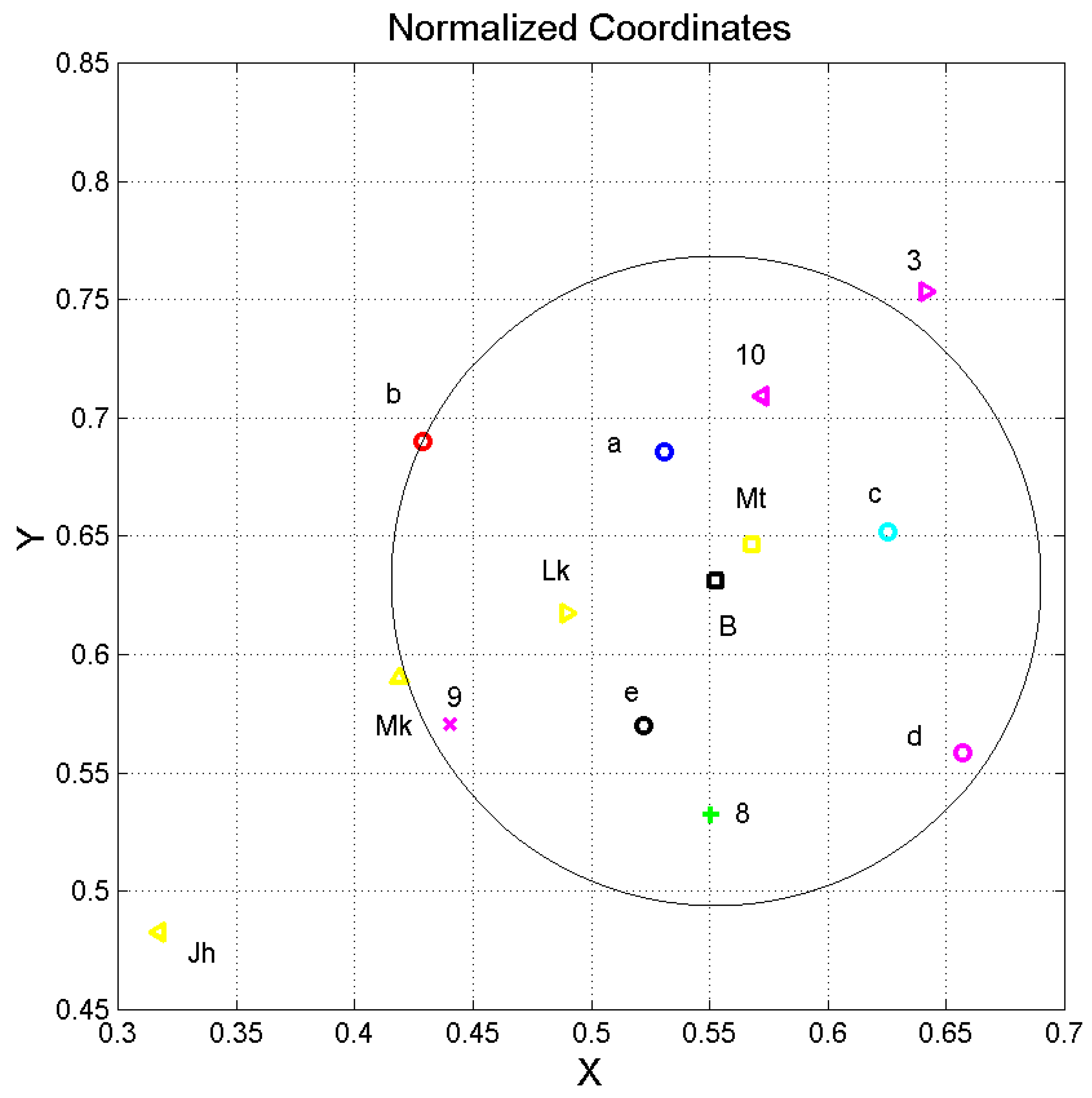
5.2. The Vector Plane

Let us consider the following six vectors of the indicated components $\overrightarrow{R_1}=(C_P,P_F$), $\overrightarrow{R_2}=(M_F,P_F$), $\overrightarrow{R_3}=(I_P,P_F$), $\overrightarrow{R_4}=(C_P,M_F$), $\overrightarrow{R_5}=(I_P,M_F$), $\overrightarrow{R_6}=(I_P,C_P$) and their resulting vector:

$$\overrightarrow{R}={{\displaystyle \sum }}_{k=1}^6\overrightarrow{R_k}$$

(19)

The choice of which parameter represents the component in the abscissa and ordinate axes is not important because, once the choice is made, the numerical results will depend on it, but not the relative comparisons and general conclusions.

Figure 2 shows the resulting vector (19). The Cartesian coordinates reported have been “normalized” so that Of Mice and Men is located at (0,0) (blue pentagon) and Moby Dick is located at (1,1) (green triangle with vertex pointing down). This normalized representation allows us to maintain the relative distances by assuming the same unit in the two coordinates.

It can be noted that, compared to the other English works, Dickens’s novels are all very near to each other, within the circle drawn from their barycenter (black square) with the radius reaching David Copperfield (red circle). It can also be noted that there is a clear distinction between XIX century (magenta and green marks) and XX century novels (blue marks), therefore introducing a time arrow in the development of the English literature, at least for the sampled works. The outlying vector (1.443, 2.211) of Robinson Crusoe (1719) is not reported due to space constraints.

Curiously, the Gospel of Matthew in the King James version of the Bible (yellow square, see Table 3) is very near to Dicken’s barycenter. This is an unexpected coincidence, which requires further investigation. Did the classical New Testament books available at that time—namely the King James translations—affect the mathematical structure of Dickens’ writings? In Section 8, we propose a likely answer to this question by considering also the other three Gospels (Mark, Luke, John).

As stated before, all these findings and observations refer to a high-level comparison because they involve only average values. In literary works, however, there are multiple communication channels [2,3], one of which is the so-called “sentences channel”, a channel that linearly links the sentences of two literary works for an equal number of words. The theory of these channels includes not only averages, such as regression lines, but also correlation coefficients, as recalled in the first part of this article; therefore, in the next section, we apply the theory to Dickens’ works.

6. Experimental Signal-to-Noise Ratio of Self- and Cross-Channels

As discussed in Section 3, we consider the values of ${\mathsf{\Gamma }}_{dB,ex}$ concerning the sentences channel.

Table 4. Slope $m$ and correlation coefficient $r$ of the regression line between the number of sentences $n_S$ (dependent variable) and the number of words $n_W$ (independent variable). Four decimal digits are reported because some values differ only from the third digit.

Literary Work	$\mathit{m}$	$\mathit{r}$
Oliver Twist	0.0417	0.9307
David Copperfield	0.0411	0.9704
Bleak House	0.0466	0.9391
A Tale of Two Cities	0.0447	0.9680
Our Mutual Friend	0.0463	0.9149
Matthew	0.0447	0.9499

lists the slope $m$and the correlation coefficient $r$ of the regression line between the number of sentences $n_s$(dependent variable) and the number of words $n_W$ (independent variable) per chapter in Dickens’ works and in Matthew. Four decimal digits are reported because some values differ only from the third digit. These data are the parameters of the input literary works $k$required by the theory.

We can notice, for example, that the slopes of Matthew and A Tale of Two Cities are equal to the forth decimal digit, but not so the correlation coefficients—recall the sensitivity of the signal-to-noise ratio to this parameter, discussed in [3]. Therefore, in this case, ${\mathsf{\Gamma }}_{dB,ex}$ is practically given by the regression noise; see Equation (8). In other words, a comparison based only on averages would conclude that the two texts are mathematically identical: only a “fine tuning” study of the sentences channel would show, as we do below, that similarity does exist but not to this extent.

Table 5. Average value $M$ (dB) and standard deviation $S$ (dB) of ${\mathsf{\Gamma }}_{dB,ex}$ (dB) in self- and cross-channels, average value and standard deviation of correlation coefficient $r_{jk}$, and slope $m_{jk}$ of the regression line between the number of sentences $n_S$ of Oliver Twist (channel output) versus the number of sentences $n_S$ in the other Dickens novels (channel input), for equal number of words, in the sentences channel. Four decimal digits are reported because some values differ only from the third digit.

Novel	$\mathbf{Signal}-\mathbf{to}-\mathbf{Noise} \mathbf{Ratio} {\mathsf{\Gamma }}_{\mathit{d}\mathit{B},\mathit{e}\mathit{x}}\left(\mathbf{dB}\right)$		$\mathbf{Correlation} \mathbf{Coefficient} {\mathit{r}}_{\mathit{j}\mathit{k}}$		$\mathbf{Slope} {\mathit{m}}_{\mathit{j}\mathit{k}}$
	$\mathit{M}$	$\mathit{S}$	Ave	Dev	Ave	Dev
Oliver Twist (self-channel)	29.45	6.66	0.9988	0.0019	1.0000	0.0151
David Copperfield	18.18	3.98	0.9904	0.0070	1.0161	0.0155
A Tale of Two Cities	17.71	2.34	0.9916	0.0064	0.9334	0.0141
Bleak House	18.92	1.31	0.9985	0.0024	0.8960	0.0136
Our Mutual Friend	19.09	1.67	0.9979	0.0025	0.9015	0.0136

shows the average value $M$ (dB) and standard deviation $S$ (dB) of ${\mathsf{\Gamma }}_{dB,ex}$ (dB) in the self- and cross-channels, the correlation coefficient $r_{jk}$, and the slope $m_{jk}$of the regression line between the number of sentences $n_S$of Oliver Twist (output channel) versus the number of sentences $n_S$ in the other Dickens novels (input channels), for an equal number of words.

Table 6. Average value $M$ (dB) and standard deviation $S$ (dB) of ${\mathsf{\Gamma }}_{dB,ex}$ (dB) in self- and cross-channels, correlation coefficient $r_{jk}$, and slope $m_{jk}$ of the regression line between the number of sentences $n_S$ of David Copperfield (channel output, self-channel) versus the number of sentences $n_S$ in the other Dickens novels (channel input, cross-channels), for equal number of words, in the sentences channel.

Novel	$\mathbf{Signal}-\mathbf{to}-\mathbf{Noise} \mathbf{Ratio} {\mathsf{\Gamma }}_{\mathit{d}\mathit{B},\mathit{e}\mathit{x}} \left(\mathbf{dB}\right)$		$\mathbf{Correlation} \mathbf{Coefficient} {\mathit{r}}_{\mathit{j}\mathit{k}}$		$\mathbf{Slope} {\mathit{m}}_{\mathit{j}\mathit{k}}$
	$\mathit{M}$	$\mathit{S}$	Ave	Dev	Ave	Dev
David Copperfield (self-channel)	32.02	6.32	0.9994	0.0009	0.9996	0.0120
Oliver Twist	17.87	2.63	0.9906	0.0045	0.9842	0.0117
A Tale of Two Cities	21.24	1.31	0.9993	0.0010	0.9191	0.0110
Bleak House	16.22	1.11	0.9933	0.0038	0.8816	0.0103
Our Mutual Friend	14.32	1.15	0.9843	0.0059	0.8874	0.0106

,

Table 7. Average value $M$ (dB) and standard deviation $S$ (dB) of ${\mathsf{\Gamma }}_{dB,ex}$ (dB) in self- and cross-channels, correlation coefficient $r_{jk}$, and slope $m_{jk}$ of the regression line between the number of sentences $n_S$ of Bleak House (channel output, self-channel) versus the number of sentences $n_S$ in the other Dickens novels (channel input, cross-channels), for equal number of words, in the sentences channel.

Novel	$\mathbf{Signal}-\mathbf{to}-\mathbf{Noise} \mathbf{Ratio} {\mathsf{\Gamma }}_{\mathit{d}\mathit{B},\mathit{e}\mathit{x}}\left(\mathbf{dB}\right)$		$\mathbf{Correlation} \mathbf{Coefficient} {\mathit{r}}_{\mathit{j}\mathit{k}}$		$\mathbf{Slope} {\mathit{m}}_{\mathit{j}\mathit{k}}$
	$\mathit{M}$	$\mathit{S}$	Ave	Dev	Ave	Dev
Bleak House (self-channel)	29.86	6.72	0.9988	0.0018	1.0007	0.0126
Oliver Twist	17.75	1.39	0.9985	0.0018	1.1175	0.0143
David Copperfield	19.57	3.55	0.9942	0.0053	1.0436	0.0133
A Tale of Two Cities	19.62	3.50	0.9943	0.0052	1.0439	0.0135
Our Mutual Friend	24.46	6.20	0.9968	0.0031	1.0075	0.0129

,

Table 8. Average value $M$ (dB) and standard deviation $S$ (dB) of ${\mathsf{\Gamma }}_{dB,ex}$ (dB) in self- and cross-channels, correlation coefficient $r_{jk}$, and slope $m_{jk}$ of the regression line between the number of sentences $n_S$ of A Tale of Two Cities (channel output, self-channel) versus the number of sentences $n_S$ in the other Dickens novels (channel input, cross-channels), for equal number of words, in the sentences channel.

Novel	$\mathbf{Signal}-\mathbf{to}-\mathbf{Noise} \mathbf{Ratio} {\mathsf{\Gamma }}_{\mathit{d}\mathit{B},\mathit{e}\mathit{x}}\left(\mathbf{dB}\right)$		$\mathbf{Correlation} \mathbf{Coefficient} {\mathit{r}}_{\mathit{j}\mathit{k}}$		$\mathbf{Slope} {\mathit{m}}_{\mathit{j}\mathit{k}}$
	$\mathit{M}$	$\mathit{S}$	Ave	Dev	Ave	Dev
A Tale of Two Cities (self-channel)	26.01	6.85	0.9974	0.0036	0.9955	0.0297
Oliver Twist	18.57	5.84	0.9921	0.0068	1.0666	0.0316
David Copperfield	19.23	2.74	0.9972	0.0039	1.0829	0.0323
Bleak House	19.72	3.39	0.9943	0.0053	0.9548	0.0281
Our Mutual Friend	16.72	3.68	0.9868	0.0096	0.9611	0.0285

and

Table 9. Average value $M$ (dB) and standard deviation $S$ (dB) of ${\mathsf{\Gamma }}_{dB,ex}$ (dB) in self- and cross-channels, correlation coefficient $r_{jk}$, and slope $m_{jk}$ of the regression line between the number of sentences $n_S$ of Our Mutual Friend (channel output, self-channel) versus the number of sentences $n_S$ in the other Dickens novels (channel input, cross-channels), for equal number of words, in the sentences channel.

Novel	$\mathbf{Signal}-\mathbf{to}-\mathbf{Noise} \mathbf{Ratio} {\mathsf{\Gamma }}_{\mathit{d}\mathit{B},\mathit{e}\mathit{x}}\left(\mathbf{dB}\right)$		$\mathbf{Correlation} \mathbf{Coefficient} {\mathit{r}}_{\mathit{j}\mathit{k}}$		$\mathbf{Slope} {\mathit{m}}_{\mathit{j}\mathit{k}}$
	$\mathit{M}$	$\mathit{S}$	Ave	Dev	Ave	Dev
Our Mutual Friend (self-channel)	29.89	6.66	0.9989	0.0017	1.0004	0.0139
Oliver Twist	18.00	1.58	0.9981	0.0028	1.1101	0.0154
David Copperfield	12.67	1.61	0.9841	0.0085	1.1272	0.0155
Bleak House	25.22	6.58	0.9968	0.0038	0.9942	0.0138
A Tale of Two Cities	15.47	2.39	0.9858	0.0078	1.0358	0.0144

show the results when the output channel is David Copperfield, Bleak House, A Tale of Two Cities, Our Mutual Friend. For example, according to Table 4, in David Copperfield, 100 words give $n_S=0.0411\times 100=4.11$ sentences on average; therefore, from Table 5, this number of sentences is “translated” into $\left(1.0161\pm 0.0155\right)\times 4.11\approx 4.18\pm 0.06$ sentences in Oliver Twist, with correlation coefficient $r_{jk}=0.9904\pm 0.0070$. Of course, the largest statistical value cannot exceed 1.

Finally, notice the asymmetry typical of linguistic channels [1,2,3,4]. For example, from Table 5, in the cross-channel of David Copperfield, ${\mathsf{\Gamma }}_{dB,ex}=18.18\pm 3.98$ (dB), while, from Table 6, in the cross-channel of Oliver Twist, ${\mathsf{\Gamma }}_{dB,ex}=17.87\pm 2.63$ (dB).

Notice that the standard deviation of ${\mathsf{\Gamma }}_{dB,ex}$ in self-channels is approximately $6~7$ dBs, independently of the average value, and when the average value $M$ of a cross-channel moves closer to that of the self-channel, also its standard deviation tends to assume the same value (e.g., Our Mutual Friend in Table 7), a typical feature of cross-channels being very similar to self-channels [2,3,4].

Now, as discussed in Section 3, self-channels can describe all possible literary works that, by maintaining the same statistical properties of the original work, the author might have written at the same time as the original one. Therefore, the closer the parameters of the cross-channels to those of the self-channel, the more similar are the input and output works. In other words, the Gaussian probability density function of a cross-channel can largely overlap with that of the self-channel. This superposition is quantified by the likeness index, as shown in [3] for ${\mathsf{\Gamma }}_{dB,ex}$. In the next section, we show this overlap for the channel capacity $C$ and calculate the likeness index.

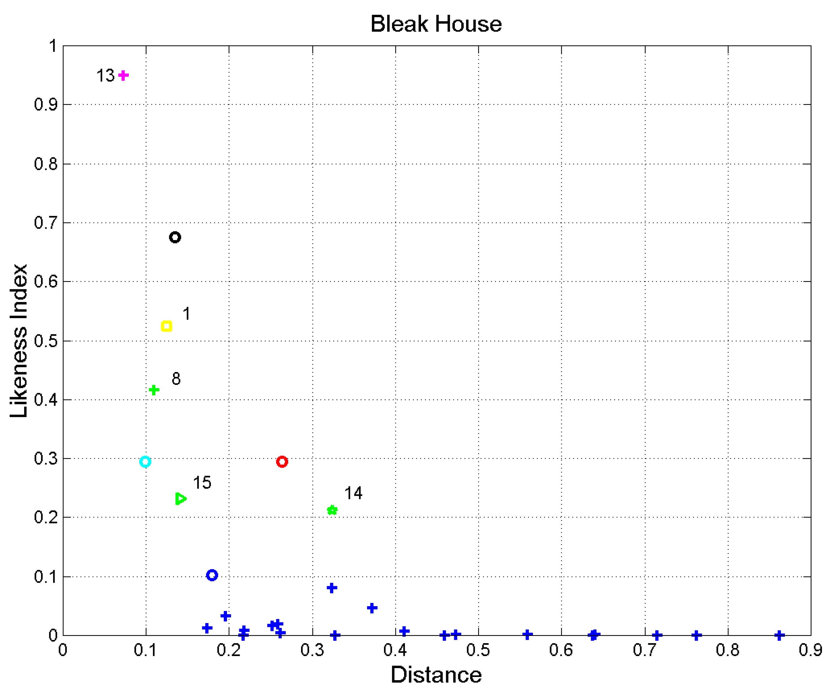
7. Capacity of Self- and Cross-Channels and Likeness Index

In this section, we calculate the capacity $C$ of self- and cross-channels. We assume that the signal-to-noise ratio ${\mathsf{\Gamma }}_{dB,ex}$ of these channels is Gaussian, with the average value and standard deviation given in Table 5, Table 6, Table 7, Table 8, Table 9 and

Table 10. Average value $M$ (dB) and standard deviation $S$ (dB) of ${\mathsf{\Gamma }}_{dB,ex}$ (dB) in self- and cross-channels, correlation coefficient $r_{jk}$, and slope $m_{jk}$ of the regression line between the number of sentences $n_S$ of Matthew (channel output, self-channel) versus the number of sentences $n_S$ in Dickens’ novels (channel input, cross-channels), for equal number of words, in the sentences channel.

Novel	$\mathbf{Signal}-\mathbf{to}-\mathbf{Noise} \mathbf{Ratio} {\mathsf{\Gamma }}_{\mathit{d}\mathit{B},\mathit{e}\mathit{x}}\left(\mathbf{dB}\right)$		$\mathbf{Correlation} \mathbf{Coefficient} {\mathit{r}}_{\mathit{j}\mathit{k}}$		$\mathbf{Slope} {\mathit{m}}_{\mathit{j}\mathit{k}}$
	$\mathit{M}$	$\mathit{S}$	Ave	Dev	Ave	Dev
Matthew (self-channel)	26.75	6.57	0.9979	0.0036	1.0008	0.0258
Oliver Twist	20.02	4.19	0.9964	0.0041	1.0721	0.0273
David Copperfield	17.71	2.74	0.9948	0.0073	1.0885	0.0281
Bleak House	23.72	6.32	0.9956	0.0064	1.0000	0.0260
A Tale of Two Cities	22.97	3.99	0.9974	0.0037	0.9596	0.0251
Our Mutual Friend	19.83	3.95	0.9934	0.0060	0.9653	0.0252

, and calculate $C$ from Equation (13), by running a Monte Carlo simulation (100,000 simulations).

Figure 3 shows the results for Bleak House (Table 7), together with the theoretical Gaussian probability density function calculated according to the approximation given by Equations (16) and (17). The simulated data show a probability density function that agrees extremely well with the theoretical model. In fact, the average value and standard deviation of the simulated data agree to the forth digit with those calculated with Equations (16) and (17), therefore confirming the validity of the hypotheses assumed for the Gaussian model, in Equation (17).

Figure 4, Figure 5, Figure 6, Figure 7 and Figure 8 show the Monte Carlo results for the channels listed in Table 5, Table 6, Table 7, Table 8 and Table 9. We see a further confirmation that the capacity of all self- and cross-channels can be very well modeled as Gaussian. This result applies also to the case in which Matthew is the output text (Figure 8). Moreover, the average value of the worst cross-channels tends to be approximately half of that of the self-channel.

In conclusion, if the stochastic variable ${\mathsf{\Gamma }}_{dB,ex}$ of a linguistic channel is Gaussian, then also its capacity (bits per symbol) is Gaussian.

Now, from the Gaussian probability density functions shown in Figure 3, Figure 4, Figure 5, Figure 6, Figure 7 and Figure 8, the likeness index $I_C$ can be calculated. As discussed in Section 4, this index coincides with the likeness index $I_L$; therefore, we do not distinguish between them in the following.

Table 11. Likeness index $I_L=I_C$ between the indicated literary works, sentences channel. The work in the first line indicates the output text; the text in the first column indicates the input text (regression line given in Table 3). For example, in the channel Our Mutual Friend$\underset{}{\to }$ Bleak House, $I_L=0.675$, while in the reverse channel, Bleak House$\underset{}{\to }$ Our Mutual Friend, $I_L=0.724$.

Novel	Oliver Twist	David Copperfield	Bleak House	A Tale of Two Cities	Our Mutual Friend	Matthew
Oliver Twist	1	0.102	0.103	0.554	0.116	0.508
David Copperfield	0.277	1	0.295	0.415	0.030	0.293
Bleak House	0.139	0.025	1	0.488	0.724	0.813
A Tale of Two Cities	0.165	0.120	0.294	1	0.097	0.671
Our Mutual Friend	0.168	0.013	0.675	0.353	1	0.483

reports the results for Dickens’ works. The title in the first line indicates the output novel, and the title in the first column indicates the input novel (regression line given in Table 4). The output novel is the work that produces the regression lines in Step 2 of the Monte Carlo simulation, and the input work (with fixed regression line, Table 4) produces the cross-channel.

For example, in the channel Our Mutual Friend$\underset{}{\to }$Bleak House, $I_L=0.675$. In the reverse channel, Bleak House$\underset{}{\to }$Our Mutual Friend, $I_L=0.724$. The meaning of these results is the following: in the channel Bleak House$\underset{}{\to }$Our Mutual Friend, the regression line between the sentences and words in every new Our Mutual Friend simulated in Step 2 of the Monte Carlo algorithm of Section 3 is very similar to that of the input text Bleak House (regression given in Table 4), so that the theory of Section 2 produces, in the end, this large $I_L$. In other words, the regression of Bleak House belongs to the set of regression lines (self-channel) of Our Mutual Friend, a “belonging” described by the two Gaussian densities and measured by $I_L=0.724$.

Now, similarly, in the channel Our Mutual Friend$\underset{}{\to }$Bleak House, the regression line between the sentences and words in every new Bleak House is quite similar to that of the input text Our Mutual Friend (Table 3), so that $I_L=0.675$. However, in this case, this asymmetry may indicate a time arrow, because Bleak House (written earlier) seems to be more “contained” in A Mutual Friend (written later) than the reverse, because $0.724>0.675$. The time arrow, however, is not evident in other cases.

It is very interesting and surprising to compare them with Matthew. It can be noticed, in fact, that Bleak House ($I_L=0.813$) and A Tale of Two Cities ($I_L=0.671$) are more similar to Matthew than the other novels. In other words, Matthew seems to have affected the statistics of the sentences in these two Dickens works more than those found in Our Mutual Friend, Oliver Twist, and David Copperfield. Appendix A reports the tables for the other Gospels.

Now, let us consider in more depth the likely influence of the Gospels of the King James translation on Dickens’ writing.

8. The Likely Influence of the Gospels on Dickens’ Novels

The very similar values of the deep language parameters in Dickens’ novels and in the Gospel according to Matthew (Figure 1 and Figure 2) may be a trace of the influence unconsciously left in Dickens’ style after researching the life of Jesus of Nazareth and writing The Life of Our Lord for his children, published only in 1934 [48]. Dickens felt the need to impart some religious instruction to his children by writing a simplified version of the Gospels. According to scholars [49,50,51], in his novels, all the strongest illustrations are derived from the New Testament because he gave priceless value to its Books.

Figure 9 shows a detail of Figure 2, with the insertion of the other Gospels, whose deep language parameters are reported in

Table 12. Gospels statistics, King James version. Number of chapters (i.e., the number of samples considered in calculating the regression lines of the theory), total number of characters contained in the words, total number of words and sentences, deep language parameters $C_P$, $P_F$, $I_P$, $M_F$, with standard deviation reported in the second line.

Gospel	Chapters	Characters	Words	Sentences	${\mathit{C}}_{\mathit{p}}$	${\mathit{P}}_{\mathit{F}}$	${\mathit{I}}_{\mathit{P}}$	${\mathit{M}}_{\mathit{F}}$
Matthew	28	99,795	23,397	1040	4.266 0.011	23.510 4.402	5.906 0.549	3.981 0.625
Mark	16	61,355	15,166	688	4.046 0.022	22.297 0.5969	5.847 0.073	3.816 0.100
Luke	24	102,726	25,469	1127	4.033 0.015	22.883 0.544	6.104 0.178	3.789 0.096
John	21	75,635	19,094	968	3.961 0.029	19.971 0.496	5.838 0.134	3.443 0.092

. Notice that only the three synoptic Gospels (Matthew, Mark, Luke) fall within the circle of Dickens’ novels, while John is clearly further away. In other words, John does not seem to have notably influenced Dickens’ writing.

Table 13. Slope $m$ and correlation coefficient $r$ of the regression line between the number of sentences $n_S$ (dependent variable) and the number of words $n_W$ (independent variable) per chapter, in the canonical Gospels. Four decimal digits are reported because some values differ only from the third digit.

Gospel	$\mathit{m}$	$\mathit{r}$
Matthew	0.0447	0.9499
Mark	0.0459	0.9541
Luke	0.0446	0.9329
John	0.0511	0.9441

reports the slope $m$and correlation coefficient $r$ of the regression line between the number of sentences $n_S$(dependent variable) and the number of words $n_W$ (independent variable) per chapter, in the Gospels. Four decimal digits are reported because some values differ only from the third digit. Notice that Matthew and Luke almost coincide, as already observed in the general study reported in [52] on the original Greek texts. Mark is not far, therefore distinguishing the synoptic Gospels from John.

Table 14. Likeness index $I_L=I_C$ between the indicated Dickens novels and the four Canonical Gospels in the King James translation (output), sentences channel. The Gospel in the first line indicates the output text; the text in the first column indicates the input text (regression line given in Table 10). For example, in the channel Our Mutual Friend$\underset{}{\to }$ Bleak House, $I_L=0.675$, while in the reverse channel, Bleak House$\underset{}{\to }$ Our Mutual Friend, $I_L=0.724$.

Input Novel	Matthew	Mark	Luke	John
Oliver Twist	0.508	0.429	0.545	0.045
David Copperfield	0.293	0.384	0.325	0.045
Bleak House	0.671	0.851	0.767	0.314
A Tale of Two Cities	0.813	0.890	0.643	0.170
Our Mutual Friend	0.483	0.641	0.707	0.227

summarizes the likeness index between the indicated Gospel (output) and Dickens’ novels (input). This table shows that Dickens’ novels have been likely influenced by the synoptic Gospels, especially the last three novels, which were written shortly after The Life of Our Lord.

In conclusion, we conjecture that the synoptic Gospels, read and studied by Dickens, affected and shaped, unconsciously, the deep language parameters of his writing style.

9. Final Remarks

We can now link the results shown in Figure 2 (vectors) with the likeness index $I_L$. We have noticed that Dickens’ novels are concentrated within a circle, which includes very few novels by other authors.

In the Cartesian plane, we can calculate the Pythagorean distance $\mathcal{l}$ between a literary work and a reference work, and correlate $\mathcal{l}$ with the corresponding $I_L$. Such an exercise is shown in Figure 10, as an example, where the reference (output) is Bleak House. It is clearly evident that $I_L$ decreases sharply as $\mathcal{l}$ increases.

For small distances ($\mathcal{l}\lesssim 0.15)$, $I_L$ and $\mathcal{l}$ show a tight inverse relationship. The closest work to Bleak House is The Jungle Book (13), followed by Little Women (8), Treasure Island (9), and The Adventures of Huckleberry Finn (10). Although these novels fall within the circle, they could not have influenced Dickens’ style because they were published later than Bleak House (Table 2 and Table 3); therefore, a small distance is a necessary but not a sufficient condition for two literary works being mathematically similar.

10. Conclusions

In the first part of the article, we have recalled our general theory of linguistic channels and have studied the Shannon capacity and interdependence of these channels. In the second part, to show some features and usefulness of the theory, we have applied it to novels written by Charles Dickens and other authors of English literature, including the Gospels of the classical King James version of the Bible.

In literary works (or in any long texts), there are multiple communication channels, one of which is the channel that linearly links the sentences of two literary works for an equal number of words, as explicitly studied in the article. The theory of these channels considers not only averages, such as regression lines, but also correlation coefficients.

A Monte Carlo simulation addresses the inaccuracy in estimating the slope and correlation coefficient of regression lines due to the small sample size (i.e., given by the number of chapters of each literary work). However, besides the usefulness of the simulation as a “renormalization” tool shown in the article, there is another very likely more interesting property concerning the new generated literary works. In fact, because the mathematical theory does not consider meaning, the simulated texts might have been “written” by the author, as they maintain the main statistical properties of the deep language parameters of the original text. In other words, they are “literary works” that the author might have written at the time that he wrote the original work.

We have shown that the probability density function of the capacity of self- and cross-channels (defined and studied in the article) is a Gaussian stochastic variable. The closer the parameters of the cross-channels are to those of the self-channel, the more similar are the two literary works. The similarity is measured by the likeness index.

We have found that Dickens’ novels show striking and unexpected mathematical/statistical similarity to the synoptic Gospels. The similarity may be a trace of the influence unconsciously left in Dickens’ deep language style after researching the life of Jesus of Nazareth and writing The Life of Our Lord for his children.

We have shown that the Pythagorean distance $\mathcal{l}$ (in a suitably defined Cartesian plane involving the deep language parameters) and the likeness index, for a reference literary work compared to all others, correlates with the corresponding likeness index with a tight inverse proportional relationship.

A similar approach can be applied, of course, to any literary corpus written in any alphabetical language, and this would allow us to compare different texts, even in translation.

References

1. Matricciani, E. Deep Language Statistics of Italian throughout Seven Centuries of Literature and Empirical Connections with Miller’s 7 ∓ 2 Law and Short-Term Memory. Open J. Stat. 2019, 9, 373–406. [Google Scholar] [CrossRef] [Green Version]
2. Matricciani, E. A Statistical Theory of Language Translation Based on Communication Theory. Open J. Stat. 2020, 10, 936–997. [Google Scholar] [CrossRef]
3. Matricciani, E. Linguistic Mathematical Relationships Saved or Lost in Translating Texts: Extension of the Statistical Theory of Translation and Its Application to the New Testament. Information 2022, 13, 20. [Google Scholar] [CrossRef]
4. Matricciani, E. Multiple Communication Channels in Literary Texts. Open J. Stat. 2022, 12, 486–520. [Google Scholar] [CrossRef]
5. Shannon, C.E. A Mathematical Theory of Communication. Bell Syst. Tech. J. 1948, 27, 379–423. [Google Scholar] [CrossRef] [Green Version]
6. Catford, J.C. A Linguistic Theory of Translation. An Essay in Applied Linguistics; Oxford University Press: Oxford, UK, 1965. [Google Scholar]
7. Munday, J. Introducing Translation Studies. Theories and Applications, 2nd ed.; Routledge: London, UK, 2008. [Google Scholar]
8. Proshina, Z. Theory of Translation, 3rd ed.; Far Eastern University Press: Manila, Philippines, 2008. [Google Scholar]
9. Trosberg, A. Discourse analysis as part of translator training. Curr. Issues Lang. Soc. 2000, 7, 185–228. [Google Scholar] [CrossRef]
10. Tymoczko, M. Translation in a Post—Colonial Context: Early Irish Literature in English Translation; St. Jerome Publishing: Manchester, UK, 1999. [Google Scholar]
11. Warren, R. (Ed.) The Art of Translation: Voices from the Field; North-Eastern University Press: Boston, MA, USA, 1989. [Google Scholar]
12. Williams, I. A corpus-based study of the verb observar in English-Spanish translations of biomedical research articles. Target 2007, 19, 85–103. [Google Scholar] [CrossRef]
13. Wilss, W. Knowledge and Skills in Translator Behaviour; John Benjamins: Amsterdam, The Netherlands; Philadelphia, PA, USA, 1996. [Google Scholar]
14. Wolf, M.; Fukari, A. (Eds.) Constructing a Sociology of Translation; John Benjamins: Amsterdam, The Netherlands; Philadelphia, PA, USA, 2007. [Google Scholar]
15. Gamallo, P.; Pichel, J.R.; Alegria, I. Measuring Language Distance of Isolated European Languages. Information 2020, 11, 181. [Google Scholar] [CrossRef] [Green Version]
16. Barbançon, F.; Evans, S.; Nakhleh, L.; Ringe, D.; Warnow, T. An experimental study comparing linguistic phylogenetic reconstruction methods. Diachronica 2013, 30, 143–170. [Google Scholar] [CrossRef] [Green Version]
17. Bakker, D.; Muller, A.; Velupillai, V.; Wichmann, S.; Brown, C.H.; Brown, P.; Egorov, D.; Mailhammer, R.; Grant, A.; Holman, E.W. Adding typology to lexicostatistics: Acombined approach to language classification. Linguist. Typol. 2009, 13, 169–181. [Google Scholar] [CrossRef]
18. Petroni, F.; Serva, M. Measures of lexical distance between languages. Phys. A Stat. Mech. Appl. 2010, 389, 2280–2283. [Google Scholar] [CrossRef] [Green Version]
19. Carling, G.; Larsson, F.; Cathcart, C.; Johansson, N.; Holmer, A.; Round, E.; Verhoeven, R. Diachronic Atlas of Comparative Linguistics (DiACL)—A database for ancient language typology. PLoS ONE 2018, 13, e0205313. [Google Scholar] [CrossRef] [Green Version]
20. Gao, Y.; Liang, W.; Shi, Y.; Huang, Q. Comparison of directed and weighted co-occurrence networks of six languages. Phys. A Stat. Mech. Appl. 2014, 393, 579–589. [Google Scholar] [CrossRef]
21. Liu, H.; Cong, J. Language clustering with word co-occurrence networks based on parallel texts. Chin. Sci. Bull. 2013, 58, 1139–1144. [Google Scholar] [CrossRef] [Green Version]
22. Gamallo, P.; Pichel, J.R.; Alegria, I. From Language Identification to Language Distance. Phys. A 2017, 484, 162–172. [Google Scholar] [CrossRef]
23. Pichel, J.R.; Gamallo, P.; Alegria, I. Measuring diachronic language distance using perplexity: Application to English, Portuguese, and Spanish. Nat. Lang. Eng. 2019, 26, 433–454. [Google Scholar] [CrossRef]
24. Eder, M. Visualization in stylometry: Cluster analysis using networks. Digit. Scholarsh. Humanit. 2015, 32, 50–64. [Google Scholar] [CrossRef]
25. Brown, P.F.; Cocke, J.; Pietra, A.D.; Pietra, V.J.D.; Jelinek, F.; Lafferty, J.D.; Mercer, R.L.; Roossin, P.S. A Statistical Approach to Machine Translation. Comput. Linguist. 1990, 16, 79–85. [Google Scholar]
26. Koehn, F.; Och, F.J.; Marcu, D. Statistical Phrase-Based Translation. In Proceedings of the 2003 Conference of the North American Chapter of the Association for Computational Linguistics on Human Language Technology (HLT-NAACL 2003), Edmonton, AB, Canada, 27 May–1 June 2003; pp. 48–54. [Google Scholar]
27. Carl, M.M.; Schaeffer, M. Sketch of a Noisy Channel Model for the Translation Process. In Empirical Modelling of Translation and Interpreting; Hansen-Schirra, S., Czulo, O., Hofmann, S., Eds.; Language Science Press: Berlin, Germany, 2017; pp. 71–116. [Google Scholar] [CrossRef]
28. Elmakias, I.; Vilenchik, D. An Oblivious Approach to Machine Translation Quality Estimation. Mathematics 2021, 9, 2090. [Google Scholar] [CrossRef]
29. Lavie, A.; Agarwal, A. Meteor: An Automatic Metric for MT Evaluation with High Levels of Correlation with Human Judgments. In Proceedings of the Second Workshop on Statistical Machine Translation, Prague, Czech Republic, 23 June 2007; pp. 228–231. [Google Scholar]
30. Banchs, R.; Li, H. AM–FM: A Semantic Framework for Translation Quality Assessment. In Proceedings of the 49th Annual Meeting of the Association for Computational Linguistics: Human Language Technologies, Portland, OR, USA, 19–24 June 2011; Volume 2, pp. 153–158. [Google Scholar]
31. Forcada, M.; Ginestí-Rosell, M.; Nordfalk, J.; O’Regan, J.; Ortiz-Rojas, S.; Pérez-Ortiz, J.; Sánchez-Martínez, F.; Ramírez-Sánchez, G.; Tyers, F. Apertium: A free/open-source platform for rule-based machine translation. Mach. Transl. 2011, 25, 127–144. [Google Scholar] [CrossRef]
32. Buck, C. Black Box Features for the WMT 2012 Quality Estimation Shared Task. In Proceedings of the 7th Workshop on Statistical Machine Translation, Montreal, QC, Canada, 7–8 June 2012; pp. 91–95. [Google Scholar]
33. Assaf, D.; Newman, Y.; Choen, Y.; Argamon, S.; Howard, N.; Last, M.; Frieder, O.; Koppel, M. Why “Dark Thoughts” aren’t really Dark: A Novel Algorithm for Metaphor Identification. In Proceedings of the 2013 IEEE Symposium on Computational Intelligence, Cognitive Algorithms, Mind, and Brain, Singapore, 16–19 April 2013; pp. 60–65. [Google Scholar]
34. Graham, Y. Improving Evaluation of Machine Translation Quality Estimation. In Proceedings of the 53rd Annual Meeting of the Association for Computational Linguistics and the 7th International Joint Conference on Natural Language Processing, Beijing, China, 26–31 July 2015; pp. 1804–1813. [Google Scholar]
35. Espla-Gomis, M.; Sanchez-Martınez, F.; Forcada, M.L. UAlacant Word-Level Machine Translation Quality Estimation System at WMT 2015. In Proceedings of the Tenth Workshop on Statistical Machine Translation, Lisbon, Portugal, 17–18 September 2015; pp. 309–315. [Google Scholar]
36. Costa-Jussà, M.R.; Fonollosa, J.A. Latest trends in hybrid machine translation and its applications. Comput. Speech Lang. 2015, 32, 3–10. [Google Scholar] [CrossRef] [Green Version]
37. Kreutzer, J.; Schamoni, S.; Riezler, S. QUality Estimation from ScraTCH (QUETCH): Deep Learning for Word-Level Translation Quality Estimation. In Proceedings of the Tenth Workshop on Statistical Machine Translation, Lisbon, Portugal, 17–18 September 2015; pp. 316–322. [Google Scholar]
38. Specia, L.; Paetzold, G.; Scarton, C. Multi-Level Translation Quality Prediction with QuEst++. In Proceedings of the ACL–IJCNLP 2015 System Demonstrations, Beijing, China, 26–31 July 2015; pp. 115–120. [Google Scholar]
39. Banchs, R.E.; D’Haro, L.F.; Li, H. Adequacy-Fluency Metrics: Evaluating MT in the Continuous Space Model Framework. IEEE/ACM Trans. Audio Speech Lang. Process. 2015, 23, 472–482. [Google Scholar] [CrossRef]
40. Martins, A.F.T.; Junczys-Dowmunt, M.; Kepler, F.N.; Astudillo, R.; Hokamp, C.; Grundkiewicz, R. Pushing the Limits of Quality Estimation. Trans. Assoc. Comput. Linguist. 2017, 5, 205–218. [Google Scholar] [CrossRef] [Green Version]
41. Kim, H.; Jung, H.Y.; Kwon, H.; Lee, J.H.; Na, S.H. Predictor-Estimator: Neural Quality Estimation Based on Target Word Prediction for Machine Translation. ACM Trans. Asian Low-Resour. Lang. Inf. Process. 2018, 17, 1–22. [Google Scholar] [CrossRef]
42. Kepler, F.; Trénous, J.; Treviso, M.; Vera, M.; Martins, A.F.T. OpenKiwi: An Open Source Framework for Quality Estimation. In Proceedings of the 57th Annual Meeting of the Association for Computational Linguistics: System Demonstrations, Florence, Italy, 28 July–2 August 2019; pp. 117–122. [Google Scholar]
43. D’Haro, L.; Banchs, R.; Hori, C.; Li, H. Automatic Evaluation of End-to-End Dialog Systems with Adequacy-Fluency Metrics. Comput. Speech Lang. 2018, 55, 200–215. [Google Scholar] [CrossRef]
44. Yankovskaya, E.; Tättar, A.; Fishel, M. Quality Estimation with Force-Decoded Attention and Cross-Lingual Embeddings. In Proceedings of the Third Conference on Machine Translation: Shared Task Papers, Belgium, Brussels, 31 October–1 November 2018; pp. 816–821. [Google Scholar]
45. Yankovskaya, E.; Tättar, A.; Fishel, M. Quality Estimation and Translation Metrics via Pre-Trained Word and Sentence Embeddings. In Proceedings of the Fourth Conference on Machine Translation, Florence, Italy, 1–2 August 2019; Volume 3, pp. 101–105. [Google Scholar]
46. Papoulis, A. Probability & Statistics; Prentice Hall: Hoboken, NJ, USA, 1990. [Google Scholar]
47. Miller, G.A. The Magical Number Seven, Plus or Minus Two. Some Limits on Our Capacity for Processing Information. Psychol. Rev. 1955, 2, 343–352. [Google Scholar]
48. Dickens, C. The Life of Our Lord; Simon & Schuster: New York, NY, USA, 1934. [Google Scholar]
49. Walder, D. Dickens and Religion; George Allen & Unwin: London, UK, 1981. [Google Scholar]
50. Hanna, R.C. The Dickens Family Gospel: A Family Devotional Guide Based on the Christian Teachings of Charles Dickens; Rainbow Publishers: Kochi, India, 1999. [Google Scholar]
51. Hanna, R.C. The Dickens Christian Reader: A Collection of New Testament Teachings and Biblical References from the Works of Charles Dickens; AMS Press: New York, NY, USA, 2000. [Google Scholar]
52. Matricciani, E.; Caro, L.D. A Deep-Language Mathematical Analysis of Gospels, Acts and Revelation. Religions 2019, 10, 257. [Google Scholar] [CrossRef] [Green Version]
Figure 1. Scatter plot between I p and P F of the literary works of Table 1 and Table 2, together with the non-linear regression line (best-fit line) that models, on average, I p versus P F for these works, Equation (1), and Miller’s bounds. Dickens’ novels are represented by the circles: The Adventures of Oliver Twist, blue; David Copperfield, red; Bleak House, magenta; A Tale of Two Cities, cyan; Our Mutual Friend, black. Matthew: yellow square. The blue crosses refer to the other works listed in Table 2. The mark on the far right refers to Robinson Crusoe.
Information 14 00068 g001
Figure 2. Normalized coordinates x   and y of the resulting vector (18) of the literary works listed in Table 1 and Table 2, normalized so that Of Mice and Men is located at the origin (0,0) and Moby Dick is located at (1,1). Dickens’ novels are represented by the circles: The Adventures of Oliver Twist, a, blue; David Copperfield, b, red; Bleak House, d, magenta; A Tale of Two Cities, c, cyan; Our Mutual Friend, e, black. Matthew: 1, yellow square. The black square B is the barycenter of Dickens’ works. The other novels are numbered according to the order reported in Table 2.
Information 14 00068 g002
Figure 3. Upper panel: Probability density histograms of self- and cross-channel capacity. Bleak House: magenta (output); The Adventures of Oliver Twist: blue; David Copperfield: red; A Tale of Two Cities; cyan; Our Mutual Friend: black. Matthew: yellow. The continuous black lines are the theoretical densities given by Equation (17). Lower panel: Probability distribution functions.
Information 14 00068 g003
Figure 4. Upper panel: Probability density histograms of self- and cross-channel capacity. The Adventures of Oliver Twist: blue (output); David Copperfield: red; Bleak House: magenta; A Tale of Two Cities; cyan; Our Mutual Friend: black. Matthew: yellow. Lower panel: Probability distribution functions.
Information 14 00068 g004
Figure 5. Upper panel: Probability density histograms of self- and cross-channel capacity. David Copperfield: red (output); The Adventures of Oliver Twist: blue; Bleak House: magenta; A Tale of Two Cities; cyan; Our Mutual Friend: black. Matthew: yellow. Lower panel: Probability distribution functions.
Information 14 00068 g005
Figure 6. Upper panel: Probability density histograms of self- and cross-channel capacity. A Tale of Two Cities; cyan (output); David Copperfield: red; The Adventures of Oliver Twist: blue; Bleak House: magenta; Our Mutual Friend: black. Matthew: yellow. Lower panel: Probability distribution functions.
Information 14 00068 g006
Figure 7. Upper panel: Probability density histograms of self- and cross-channel capacity. Our Mutual Friend: black (output); A Tale of Two Cities; cyan; David Copperfield: red; The Adventures of Oliver Twist: blue; Bleak House: magenta; Matthew: yellow. Lower panel: Probability distribution functions.
Information 14 00068 g007
Figure 8. Upper panel: Probability density histograms of self- and cross-channel capacity. ; Matthew: yellow (output); Our Mutual Friend: black; A Tale of Two Cities; cyan; David Copperfield: red; The Adventures of Oliver Twist: blue; Bleak House: magenta. Lower panel: Probability distribution functions.
Information 14 00068 g008
Figure 9. Normalized coordinates x   and y of the resulting vector (18) of the literary works listed in Table 1 and Table 2 (detail) and the canonical Gospels (Matthew, Mark, Luke, John, yellow marks), normalized so that Of Mice and Men is located at the origin (0,0) and Moby Dick is located at (1,1). Dickens’ novels are represented by the circles: The Adventures of Oliver Twist, a, blue; David Copperfield, b, red; Bleak House, d, magenta; A Tale of Two Cities, c, cyan; Our Mutual Friend, e, black. The other novels are numbered according to the order reported in Table 2.
Information 14 00068 g009
Figure 10. Likeness index   I L versus Pythagorean distance l between a literary work and a reference (output) work (Bleak House).
Information 14 00068 g010