Research on Traffic Congestion Forecast Based on Deep Learning

Abstract

In recent years, the rapid economic development of China, the increase of the urban population, the continuous growth of private car ownership, the uneven distribution of traffic flow, and the local congestion of the road network have caused traffic congestion. Traffic congestion has become an inevitable problem in the process of urban development, bringing hazards and hidden dangers to citizens’ travel and urban development. The management of traffic congestion first lies in the accurate completion of the identification of road traffic status and the need to predict road congestion in the city, so as to improve the use rate of urban infrastructure road facilities and better alleviate road congestion. In this study, a deep spatial and temporal network model (DSGCN) for predicting traffic congestion status is proposed. First, our study divides the traffic network into grids, where each grid represents a different independent region. In this paper, the centroids of the grid regions are abstracted as nodes, and the dynamic correlations between the nodes are expressed in the form of adjacency matrix. Then, Graph Convolutional Neural Network is used to capture the spatial correlation between regions and a two-layer long and short-term feature model (DSTM) is used to capture the temporal correlation between regions. Finally, the DSGCN outperforms other baseline models and has higher accuracy for traffic congestion prediction as demonstrated by experiments on real PeMS datasets.

1. Introduction

In recent years, with the continuous development of social economy and increasing urban population, traffic congestion has become an important factor troubling urban development. Traffic road congestion not only brings people lower travel efficiency and higher travel cost, but also causes energy waste and air pollution due to higher fuel consumption. Accurate prediction of traffic congestion can help people to travel efficiently and reduce the waste of resources.

At present, the main methods for traffic congestion prediction at home and abroad are based on neural network prediction [1,2,3,4], support vector machine (SVM) prediction [5,6], deep learning prediction [6,7,8,9,10], etc. Vlahogianni et al. [11] proposed a neural network approach to obtain both spatial and temporal features to predict short-time traffic data. The algorithms they propose are predicted using a time period, but real traffic data are different every day, and considering only the data of adjacent time periods for prediction, the prediction results are very different from the actual data. Lu et al. [12] proposed an improved SVM algorithm based on a weighting algorithm to predict traffic congestion in cities by assigning different weights to each feature. To address the problems of existing traffic congestion prediction methods in which the predicted results differ greatly from the actual data and the predicted data set is small. In this paper, a deep spatial and temporal network model (DSGCN) for traffic congestion prediction based on deep learning [13,14,15,16,17,18,19,20] is proposed. The model is mainly used for the prediction of time-series traffic flow in urban areas. The main contributions of this study are as follows.

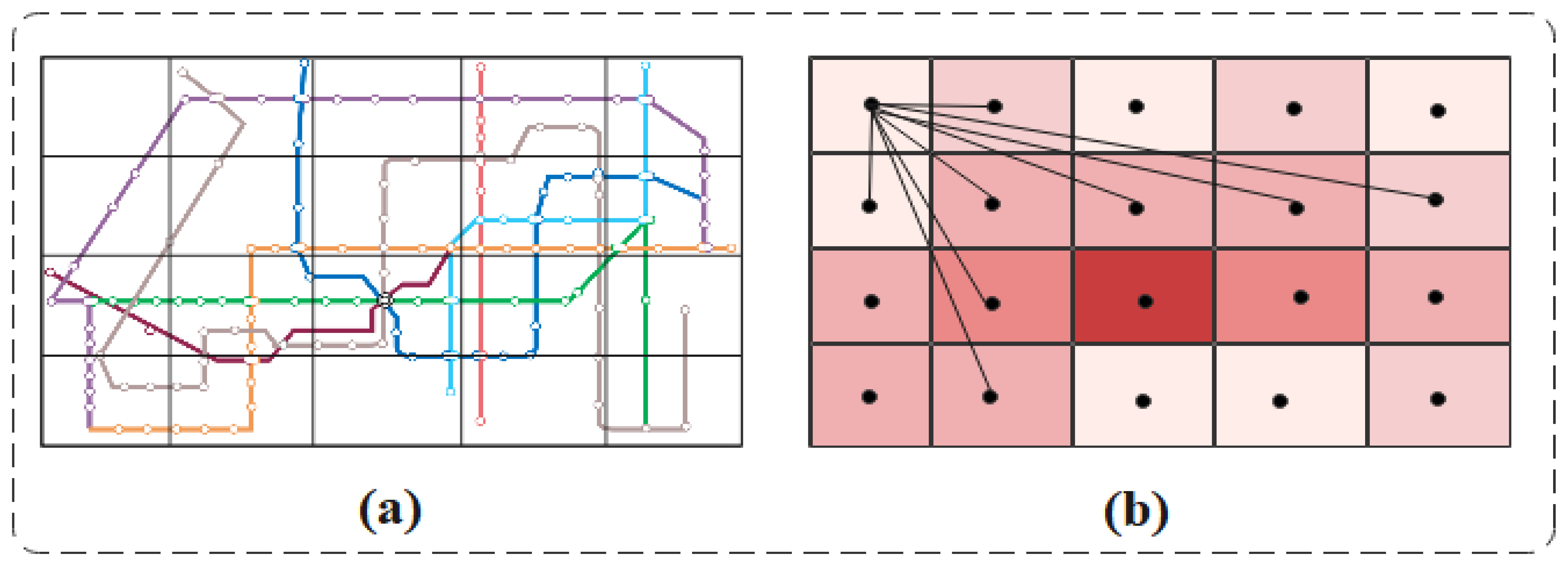
• Unlike the previous division of cities into equal-sized grids, we divide the transportation network into grids based on the attributes to which urban area belongs. Each grid represents an independent region. In this paper, the centroids of the grid are abstracted as nodes and the adjacency matrix is used to represent the spatial correlation between the nodes.
• In this study, a DSGCN model is designed to accomplish the traffic congestion prediction task. DSGCN consists of two important parts. The first part is an optimized graph convolutional neural network module that can obtain better spatial features. The second part is a two-layer DSTM unit, which allows better sequential learning of long-term and short-term temporal features.
• In this paper, experimental validation is performed on the PeMS dataset. The results show that DSGCN cannot only adequately calculate the time dependence, but can also enhance the spatial correlation of nodes in the traffic network. Meanwhile, the prediction effect of the DSGCN model proposed in this study is better than the existing baseline.

2. Related Work

Traffic congestion has a direct or indirect impact on a country’s economy and the health of its inhabitants. Ensuring economic growth and the comfort of road users are two requirements for the development of a country, so traffic congestion forecasting is gaining increased attention from government agencies. With the increase of data volume and complexity, regression models [21,22] are used less and less in traffic congestion prediction. The main idea of support vector machine (SVM) is to map nonlinear data to a high-dimensional linear space where the data can be linearly classified by hyperplanes. Tseng et al. [23] used support vector machines to determine the driving speed when predicting real-time congestion, but the increase in training data during the training process improved the accuracy and computation time, which made it difficult to perform real-time congestion prediction. Zhang et al. [24] applied the spatio-temporal feature selection algorithm (STFSA) to traffic flow sequence data to select a subset of features as the input matrix. They introduced an attention mechanism layer between the LSTM and the prediction layer, and the attention layer mechanism extracts features from the traffic flow data sequences to capture the traffic congestion state. However, this algorithm does not guarantee optimality for traffic congestion prediction considering its heuristics, biases, and trade-offs. Di et al. [25] introduced convolution to provide input to the LSTM model to form the CPM-ConvLSTM model. The graph convolutional neural network (GCN) applies spectral convolution to learn structural dependencies and feature information. Zhao et al. [26] proposed a new neural network, the traffic prediction time-graph convolutional network (T-GCN), which uses GCN to capture the static spatial features of the traffic network and designs a gated recursive unit to capture the dynamic temporal features of traffic data. However, T-GCN does not fully use the spatial information of traffic flow. Guo et al. [27] proposed an attention-based spatio-temporal graph convolutional network (ASTGCN) to enhance the dynamic spatio-temporal correlation of spatio-temporal data of traffic data while capturing spatial features using graph convolution and commonly describing temporal features using standard convolution. Yu et al. [28] proposed a new neural network approach, the spatio-Temporal Graph Convolutional Network (STGCN), for traffic prediction tasks. The architecture consists of multiple spatio-temporal convolutional blocks. The spatio-temporal convolutional blocks combine graph convolution and gated temporal convolution to extract the most useful spatial features and capture the most essential temporal features. However, the STGCN model consists entirely of convolutional structures, which are parallelized at input and slow to train with many parameters. To address the above problems, this paper designs a DSGCN model to accomplish the traffic congestion prediction task.

3. Methodology

The structure of the DSGCN model proposed in this study is shown in Figure 1. DSGCN mainly consists of GCN and two layers of DSTM, which can handle complex time-dependent and spatial dependencies. First, the input data are processed by GCN to capture the spatial features of traffic data. Second, the two-layer DSTM can capture the temporal features of traffic data and can have better adaptability with time changes. At each time slice, the DSTM can analyze the temporal correlation of traffic congestion more accurately. Finally, the fully connected layer is used to calculate the predicted values.

3.1. Data Definition

3.1.1. Problem Definition

For the task of traffic congestion prediction in complex traffic networks. First, this study divides the traffic network into independent grids, abstracts the centroids of the grids into nodes, and uses the adjacency matrix to represent the spatial correlation between the nodes. Second, this article uses the optimized graph convolutional neural network to capture the spatial features of the traffic network. Finally, a two-layer DSTM is used to capture the temporal characteristics of the traffic network and achieve the prediction of traffic congestion. The above process can be abstracted as Equation (1). Where$\mathrm{X}$ denotes historical traffic congestion data,$\mathrm{A}$ denotes the grid matrix of area division, and $\mathrm{Y}$denotes the prediction result of future traffic congestion. $\mathrm{F}$ denotes the modeling process of the GSDCN model.

$$\mathrm{Y}=\mathrm{F}\left(\mathrm{X},\mathrm{A}\right)$$

(1)

3.1.2. Grid Division Method

It is not suitable for global traffic congestion prediction when data are collected only from highways, streets, etc. Therefore, in this article, the traffic network is divided into grids, and each grid represents an independent area. As shown in Figure 2a. In this article, the center points of the grid are abstracted as nodes. As shown in Figure 2b.

In this paper, the traffic data will be transformed into graphically structured data based on the distance of nodes. $\mathrm{G}=\left(\mathrm{V},\mathrm{E},\mathrm{A}\right)$, where $\mathrm{V}$ denotes the set of all nodes and$\mathrm{E}$ is the set of distances between nodes. $\mathrm{A}\in R^N$ is the adjacency matrix constructed by calculating the distance between two nodes based on longitude and latitude. The adjacency matrix can reflect the spatial-based regional relationship information to a certain extent; the smaller the distance, the stronger the correlation between two points. The process of calculating the distance between two nodes by latitude and longitude is demonstrated in Equation (2).

$$d=R\ast arcos\left[\cos \left(Y_1\right)\ast \cos \left(Y_2\right)\ast \cos \left(X_1-X_2\right)+sin\left(Y_1\right)\ast sin\left(Y_2\right)\right]$$

(2)

where $d$ denotes the distance between two nodes. $R$ is the radius of the earth. $Y_1$ is the latitude of node 1, $Y_2$ is the latitude of node 2, $X_1$ is the longitude of node 1, and $X_2$ is the longitude of node 2. The distances between all the nodes form the adjacency matrix $\mathrm{A}$. This is shown in Figure 3.

3.2. Input and Output Definitions

As shown in Figure 4. In the prediction traffic congestion problem, the future traffic congestion data depends on the traffic congestion data in the past time slices. Suppose that predicting the number of traffic congestions at time step $t_p$ and all nodes beyond, the input data are defined in this paper as shown in Equation (3). The output data are defined as shown in Equation (4). Where$S$ is the size of the time step and $N$is the total number of all nodes.

$$X_{In}=\left\{X_{t_p-s},X_{t_p-s+1},\dots ,X_{t_p-1}\right\}ϵR^{N\times S}$$

(3)

$$Y_{out}=\left\{Y_{t_p},Y_{t_p+1},\dots ,Y_{t_p+s-1}\right\}ϵR^{N\times S}$$

(4)

3.3. Spatial Feature Extraction

In this study, we capture features for the spatial features of the data after grid division, and we capture spatial features using a graph convolutional neural network after grid division, and this article optimizes the graph convolutional neural network. In the spectral domain graph convolutional neural method, the graph structure is represented by its corresponding Laplacian matrix. First, in this paper, the grid matrix is transformed into a Laplace matrix as shown in Equation (5). Where $A$ is the adjacency matrix, the degree matrix $\mathrm{D} \mathrm{\in } R^{N\times N}$ is the diagonal matrix, and $I_n$ is the unit matrix. In addition, using the real symmetric and semi-positive properties of the regularized Laplacian matrix, it is decomposed into as shown in Equation (6).

$$L=I_n-D^{-\frac{1}{2}}A{D}^{-\frac{1}{2}}$$

(5)

$$L=U\Lambda U^T$$

(6)

where $\Lambda =\mathrm{diag}\left(\left[{\lambda }_0,\dots ,{\lambda }_{N-1}\right]\right)$ denotes the diagonal moment and $U$ is the Fourier basis. In graph convolution, the signal of the graph is a feature vector consisting of various nodes, which can be represented as $\mathrm{X}\in R^N$,where $X_i$ denotes the i-th node. The graph convolution operation is shown in Equation (7).$f\left(x\right)$ denotes the Fourier transform and $g\in R^N$ denotes the graph convolution kernel, which is the basic principle of the spectral domain graph convolution.

$$X\ast G_g=f^{-1}\left(f\left(X\right)\odot f\left(g\right)\right)=U\left(U^{T}X\odot U^{T}g\right)$$

(7)

When the number of nodes in the traffic network is large, the time complexity of the Laplace matrix eigen decomposition is large, leading to a decrease in the training effect of the model. Therefore, in this article, Chebyshev polynomials are used to approximate this problem effectively, as shown in Equations (8) and (9).

$$L\left(x\right)={\displaystyle \sum }_{k=0}^{k-1}{\theta }_k{T}_k\left(\tilde{L}\right)x$$

(8)

$$\tilde{L}=\frac{2}{{\lambda }_{max}}L-I_n$$

(9)

where $\Theta$ is a vector of polynomial coefficients.${\lambda }_{max}$ denotes the maximum eigenvalue of the Laplace matrix The recursive definition of the Chebyshev polynomial is shown in Equation (10). where $T_0\left(x\right)=1,T_1\left(x\right)=x$. In this article, the kernel is approximated as a truncated expansion of order k − 1 using the Chebyshev polynomial $T_k\left(x\right)$.

$$T_k\left(x\right)=2\times T_{k-1}\left(x\right)-T_{k-2}\left(x\right)$$

(10)

3.4. Time Feature Extraction

To capture the long-term and short-term time dependence of traffic data, a DSTM model is proposed in this article. the DSTM model can capture the temporal features, while the model can avoid the problem of gradient explosion during the training process. First, three stages are obtained by splicing training using the current input $X_t$ of the DSTM and $h_{t-1}$ passed down from the previous state. The long-term feature capture phase, the short-term feature capture phase, and the long-term and short-term feature fusion phase are used, respectively. The long-term feature capture phase is mainly used to update the long-term temporal features of the traffic data. The short-term feature capture phase updates the short-term temporal features for the input $X_t$. The long-term and short-term feature fusion phase updates the long-term and short-term temporal features of the input traffic data.

$$l_t=\sigma \left(W_f·\left[h_{t-1},X_t\right]+b_f\right)$$

(11)

$$m_t=\sigma \left(W_i·\left[h_{t-1},X_t\right]+b_i\right)$$

(12)

$$s_t=\sigma \left(W_o·\left[h_{t-1},X_t\right]+b_o\right)$$

(13)

$$\widetilde{C_t}=\sigma \left(W_c·\left[h_{t-1},X_t\right]+b_c\right)$$

(14)

As shown in Equations (11)–(14), the information $l_t$ obtained from the long-term feature capture phase, the information $m_t$ obtained from the long-term and short-term feature fusion phase, and the information $s_t$ obtained from the short-term feature capture phase are all converted to values between 0 and 1 by a sigmoid activation function after multiplying the splicing vector by the weight matrix as a kind of feature capture phase. In addition, $\widetilde{C_t}$ is the result will be converted to a value between −1 and 1 by a tanh activation function. The formula for calculating the long and short memories of DSTM is shown in Equations (15) and (16).

$$C_t=f_t\ast C_{t-1}\ast \left(1-i_t\right)+\widetilde{C_t}$$

(15)

$$h_t=\left(1-o_t\right)\ast tanh\left(C_t\right)$$

(16)

As shown in Figure 5, the DSTM cell structure accepts two inputs, namely the output value $h_{t-1}$ at the previous moment and the input value $X_t$ at the current moment, from which the two parameters enter the long-term feature capture phase and update the long-term temporal features of the traffic data to obtain the information $l_t$. Then we enter the long and short term feature fusion phase to obtain the information $m_t$ that determines the information to be updated and the cell state $\widetilde{C_t}$at the current moment. Then enter the short-term feature capture stage to update the short-term temporal features of the traffic data to the information $s_t$. Finally, the output values from these three stages are combined to obtain the long-time $C_t$short-time $h_t$ information, and finally the storage operation and the input to the next neuron.

4. Experimental Section

4.1. Data Preparation

The dataset selected for this paper is a traffic dataset on California highways in the United States. The dataset is open to the public for download. PeMS is an Archived Data User Service (ADUS) that provides more than a decade of historical analysis data. The system contains more than 44,681 detectors that cover the freeway system in all major cities in California, reporting data every 30 s, and once the compilation of a 30-s data set is complete, without any gaps, the data are aggregated into 5-min increments. We randomly select 141 detectors among multiple detectors to be abstracted as nodes of the traffic network. For these 141 nodes, 5 min of traffic data from 1 April 2021 to 25 April 2021 are selected as time slices for node data collection, for a total of 7200 time slices. The dataset is normalized by zero mean and 80% of the dataset is set as the training set and 20% of the dataset is set as the validation set.

4.2. Experimental Setup

All experiments were implemented on Windows 10 (CPU: Intel(R) Xeon(R) W-2133 [email protected] GHz; GPU: NVIDIA GeForce RTX 2080 Ti) using Python and Pytorch 1.9.0. During the training period, the batch size is set to 32, the learning rate is 0.001, and the decay parameter is set to 0.9. We use the Adam optimizer for model optimization with a convolution kernel of size 3 × 3. We repeated the experiment five times and reported the average values for different runs to obtain the optimal parameters.

In this article, we choose the mean absolute error MAE, root mean square error RMSE and mean absolute percentage error MAPE as the evaluation metrics of the experimental results. In this paper, five baseline models are set up to validate the performance of the models. All models are trained and evaluated on the same dataset. The experimental results are the average of multiple training and evaluation results, and the model structure of each baseline in the experiment is as follows.

• CNN: One convolutional layer can describe the short distance dependence of spatial regions well, while two convolutional layers can further describe the long-distance dependence.
• LSTM: A special type of RNN model. By adding input gates, forgetting gates, and output gates to control the transmission state of data, long-time memory is preserved, and unimportant information is forgotten compared with RNN.
• ConvLSTM: With the time-series modeling function of LSTM, it can also capture local features by CNN, so it can learn the spatio-temporal features of spatio-temporal data.
• T-GCN: This model combines a GCN and a gated recursive unit GRU. the GCN is used to learn complex topologies to capture spatial dependencies and the GRU is used to learn dynamic changes in traffic data to capture temporal features.
• STGCN: STGCN consists of two temporal graph convolution blocks (ST-Conv Block) and one output fully connected layer (Output Layer). The spatio-temporal convolution block consists of two temporal gated convolutions and a spatial graph convolution. The spatio-temporal dependence is modeled by graph convolution and gated convolution.

4.3. Quantitative Experimental Analysis

In this experiment, we perform initial screening and denoizing of the traffic flow data and select data with true values that do not have zero values. We compared the prediction results of the DSGCN model with those of the five baseline models.

Table 1. Results of the evaluation of the DSGCN model and other baseline method models in the dataset at 15 min.

Model	MAE	RMSE	MAPE
CNN	44.35	55.24	36.89%
LSTM	36.44	50.23	28.56%
ConvLSTM	20.26	27.85	16.93%
T-GCN	17.53	26.97	13.87%
STGCN	11.81	19.87	12.49%
DSGCN	9.98	16.63	9.35%

,

Table 2. Results of the evaluation of the DSGCN model and other baseline method models in the dataset at 30 min.

Model	MAE	RMSE	MAPE
CNN	44.52	55.49	37.24%
LSTM	35.86	49.91	28.25%
ConvLSTM	20.78	28.34	17.19%
T-GCN	18.26	27.13	14.13%
STGCN	12.16	20.03	12.67%
DSGCN	11.39	17.39	10.11%

and

Table 3. Results of the evaluation of the DSGCN model and other baseline method models in the dataset at 45 min.

Model	MAE	RMSE	MAPE
CNN	44.84	55.68	37.41%
LSTM	34.98	49.32	27.91%
ConvLSTM	21.03	28.53	17.63%
T-GCN	19.23	27.65	14.30%
STGCN	13.08	20.25	13.12%
DSGCN	10.76	17.16	9.82%

show the prediction results of the DSGCN model and the other baseline method models at 15, 30, and 45 min of the data set, respectively. From Table 1, Table 2 and Table 3, it can be seen that CNN and LSTM are less effective in predicting highly discrete traffic flow data, with mean values of MAE up to 44.57 and 35.76, respectively, mean values of RMSE up to 55.47 and 49.82, respectively, and mean values of MAPE up to 37.18% and 28.24%, respectively. CNN and LSTM are the basic deep learning models, CNN is commonly used for spatial sequence modeling and LSTM is commonly used for time-series modeling. However, if they are used to model complex traffic data with many influencing factors, just modeling spatial correlation or temporal correlation cannot fit the data, so the prediction results of these two models are the worst among all models. Compared with the CNN model, the MAE of ConvLSTM was reduced by 53.57% on average and the RMSE was reduced by 49.08% on average. Compared with the evaluation parameters of LSTM, the MAE of ConvLSTM is reduced by 42.14% on average and the RMSE is reduced by 43.31% on average. Although the prediction effect of ConvLSTM was partially improved, the spatial dependence of the acquired data and its irregularity prevented the CNN from effectively extracting spatial features, and thus the prediction results were not satisfactory.

T-GCN adds GRU to the GCN to extract time-series features. Compared with the ConvLSTM model, the MAE of T-GCN decreased by 11.35% on average and the RMSE decreased by 3.51% on average. STGCN uses a spatio-temporal convolutional block consisting of two layers of sequential network and one layer of GCN, which can extract spatio-temporal correlations in different dimensions, so the feature extraction is more effective. As a result, the MAE decreased by an average of 32.66% and the RMSE decreased by an average of 26.42% compared to the T-GCN. Its prediction performance is the best among the five baseline models. DSGCN fully considers the spatio-temporal correlation between traffic speed and the factors influencing the geographic structure of the road. The GCN is used to obtain spatial features and the two-layer DSTM to obtain temporal features. From Table 1, Table 2 and Table 3, it can be seen that DSGCN has the best prediction performance with an average improvement of 13.27%, 14.9%, and 38.07% in MAE, RMSE, and MAPE metrics, respectively, compared to STGCN. The experimental results fully demonstrate the effectiveness of the model structure design.

4.4. Qualitative Experimental Analysis

In this experiment, we evaluate the state of traffic congestion by normalizing the traffic flow data so that the data are limited to the range (0, 1). The line graphs represent the degree of fit of the DSGCN and baseline models to the real data, and the effectiveness of the models in predicting traffic congestion is reflected according to the degree of fit. The scatter plot compares the difference between DSGCN and baseline models with the real data to predict congestion, where the diagonal line of the scatter plot indicates the state in which the predicted data are consistent with the real data, as shown in Figure 6 and Figure 7. From (a), we can see that the prediction results of LSTM and CNN show a huge gap with the real data, and for intervals with continuous fluctuations, LSTM and CNN show underfitting problems. CNN can describe the short distance dependence of spatial regions well, but cannot capture the temporal features of the data. While LSTM can be effectively used to train the time-series of data to obtain the temporal features of the data, they lack the design phase of spatial structure to obtain the spatial features of the data. From (b), we can see that the prediction results of CNN and LSTM models cannot fully fit the real traffic congestion data.

Compared with CNN and LSTM models, the essence of ConvLSTM is the same as LSTM, using the output of the previous layer as the input of the next layer. The difference lies in the addition of convolutional operations to obtain the temporal features of the data with the time-series modeling function of LSTM and capture the spatial local features by CNN. As shown in Figure 8, ConvLSTM can initially fit the trend of congestion data better, but the fit becomes worse over time.

The prediction results of DSGCN compared with T-GCN and STGCN are shown in Figure 9 and Figure 10, respectively. the T-GCN model uses GCN to obtain spatially correlated features between nodes in a graph structure. the T-GCN uses the gated recursive unit GRU to learn the dynamic changes in traffic data to capture the temporal dependencies. Although GCN can achieve feature extraction of irregular spatial structure by spectral domain transformation, GCN is not sufficient to extract temporal features. Therefore T-GCN joins GRU to extract time-series features. As shown in Figure 9, T-GCN can show a good degree of dispersion at small-scale aggregation points, but it is a poor fit for traffic congestion data with peaks. The degree of fit of the scatter plot is not satisfactory. STGCN includes a time-domain gating transformation module based on a one-dimensional convolution and gating mechanism and a GCN-based space-domain graph transformation module. Spatio-temporal correlations in different dimensions can be extracted, so feature extraction is more effective. From Figure 10, we can see that the prediction results of STGCN show a better advantage in each interval, but it also only predicts the general trend of traffic congestion changes, and the fitting of some details is not accurate. DSGCN can accurately predict congestion data with high dispersion by considering the temporal and spatial characteristics of traffic congestion data. The comparison of the prediction results in Figure 6, Figure 7, Figure 8, Figure 9 and Figure 10 shows that the model in this paper fits the traffic congestion data more accurately.

5. Conclusions

In this paper, we propose a traffic congestion prediction model DSGCN based on spatio-temporal feature learning. The proposed model takes into account the independent regions of the city, and the traffic network is divided into grids, each grid represents an independent region. The DSGCN takes into account both temporal and spatial characteristics of the traffic network. We use an optimized graph convolutional neural network to capture the spatial features of the traffic network and a two-layer DSTM to capture the temporal features of the traffic network. Experimental evaluation results show that our model enhances the spatial correlation features of traffic data while ensuring adequate computation of temporal dependence. Meanwhile, our proposed DSGCN model outperforms the existing baseline in prediction. In the future, we will consider other types of traffic data and use all these data to generate more types of traffic congestion forecasts. Thus, the generalization of the prediction model is enhanced and the applicability of the algorithm is further improved.

References

1. Li, Z.; Liu, F.; Yang, W.; Peng, S.; Zhou, J. A Survey of Convolutional Neural Networks: Analysis, Applications, and Prospects. In IEEE Transactions on Neural Networks and Learning Systems; IEEE: Piscataway, NJ, USA, 2021; pp. 1–21. [Google Scholar]
2. Katz, G.; Huang, D.A.; Ibeling, D.; Julian, K.; Lazarus, C.; Lim, R.; Shah, P.; Thakoor, S.; Wu, H.; Zeljić, A.; et al. The Marabou Framework for Verification and Analysis of Deep Neural Networks. In Computer Aided Verification; Springer International Publishing: Cham, Switzerland, 2019; pp. 443–452. [Google Scholar]
3. Samek, W.; Montavon, G.; Lapuschkin, S.; Anders, C.J.; Müller, K.R. Explaining Deep Neural Networks and Beyond: A Review of Methods and Applications. Proc. IEEE 2021, 109, 247–278. [Google Scholar] [CrossRef]
4. Fang, W.; Zhuo, W.; Yan, J.; Song, Y.; Jiang, D.; Zhou, T. Attention meets long short-term memory: A deep learning network for traffic flow forecasting. Phys. A Stat. Mech. Its Appl. 2022, 587, 126485. [Google Scholar] [CrossRef]
5. Sahoo, K.S.; Tripathy, B.K.; Naik, K.; Ramasubbareddy, S.; Balusamy, B.; Khari, M.; Burgos, D. An Evolutionary SVM Model for DDOS Attack Detection in Software Defined Networks. IEEE Access 2020, 8, 132502–132513. [Google Scholar]
6. Al-Qatf, M.; Lasheng, Y.; Al-Habib, M.; Al-Sabahi, K. Deep Learning Approach Combining Sparse Autoencoder with SVM for Network Intrusion Detection. IEEE Access 2018, 6, 52843–52856. [Google Scholar] [CrossRef]
7. Lv, Z.; Li, J.; Dong, C.; Li, H.; Xu, Z. Deep learning in the COVID-19 epidemic: A deep model for urban traffic revitalization index. Data Knowl. Eng. 2021, 135, 101912. [Google Scholar] [CrossRef]
8. Tian, C.; Fei, L.; Zheng, W.; Xu, Y.; Zuo, W.; Lin, C.W. Deep learning on image denoising: An overview. Neural Netw. 2020, 131, 251–275. [Google Scholar]
9. Lv, Z.; Li, J.; Dong, C.; Wang, Y.; Li, H.; Xu, Z. DeepPTP: A Deep Pedestrian Trajectory Prediction Model for Traffic Intersection. KSII Trans. Internet Inf. Syst. 2021, 15, 2321–2338. [Google Scholar]
10. Huang, B.; Ge, L.; Chen, G.; Radenkovic, M.; Wang, X.; Duan, J.; Pan, Z. Nonlocal graph theory based transductive learning for hyperspectral image classification. Pattern Recognit. 2021, 116, 107967. [Google Scholar]
11. Vlahogianni, E.I.; Karlaftis, M.; Golias, J. Optimized and meta-optimized neural networks for short-term traffic flow prediction: A genetic approach. Transp. Res. Part C Emerg. Technol. 2005, 13, 211–234. [Google Scholar]
12. Lu, J.; Chen, S.; Wang, W.; Van Zuylen, H. A hybrid model of partial least squares and neural network for traffic incident detection. Expert Syst. Appl. 2012, 39, 4775–4784. [Google Scholar] [CrossRef]
13. Xu, Z.; Lv, Z.; Li, J.; Shi, A. A Novel Approach for Predicting Water Demand with Complex Patterns Based on Ensemble Learning. Water Resour. Manag. 2022, 36, 4293–4312. [Google Scholar]
14. Xu, Z.; Lv, Z.; Li, J.; Sun, H.; Sheng, Z. A Novel Perspective on Travel Demand Prediction Considering Natural Environmental and Socioeconomic Factors. IEEE Intell. Transp. Syst. Mag. 2022, 15, 2–25. [Google Scholar] [CrossRef]
15. Lv, Z.; Li, J.; Li, H.; Xu, Z.; Wang, Y. Blind Travel Prediction Based on Obstacle Avoidance in Indoor Scene. Wirel. Commun. Mob. Comput. 2021, 2021, 5536386. [Google Scholar]
16. Liang, Y.; Li, Y.; Guo, J.; Li, Y. Resource Competition in Blockchain Networks Under Cloud and Device Enabled Participation. IEEE Access 2022, 10, 11979–11993. [Google Scholar] [CrossRef]
17. Zhao, A.; Dong, J.; Li, J.; Qi, L.; Zhou, H. Associated Spatio-Temporal Capsule Network for Gait Recognition. IEEE Trans. Multimed. 2022, 24, 846–860. [Google Scholar]
18. Zhao, A.; Li, J.; Ahmed, M. SpiderNet: A spiderweb graph neural network for multi-view gait recognition. Knowl. Based Syst. 2020, 206, 106273. [Google Scholar] [CrossRef]
19. Zhao, A.; Wang, Y.; Li, J. Transferable Self-Supervised Instance Learning for Sleep Recognition. IEEE Trans. Multimed. 2022, 1. [Google Scholar] [CrossRef]
20. Zhang, X.; Liu, W.; Waller, S.T.; Yin, Y. Modelling and managing the integrated morning-evening commuting and parking patterns under the fully autonomous vehicle environment. Transp. Res. Part B Methodol. 2019, 128, 380–407. [Google Scholar] [CrossRef]
21. Wang, H.; Liu, L.; Dong, S.; Qian, Z.; Wei, H. A novel work zone short-term vehicle-type specific traffic speed prediction model through the hybrid EMD–ARIMA framework. Transp. B Transp. Dyn. 2015, 4, 159–186. [Google Scholar] [CrossRef]
22. Ding, Q.Y.; Wang, X.F.; Zhang, X.Y.; Sun, Z.Q. Forecasting Traffic Volume with Space-Time ARIMA Model. Adv. Mater. Res. 2010, 156–157, 979–983. [Google Scholar]
23. Tseng, F.H.; Hsueh, J.H.; Tseng, C.W.; Yang, Y.T.; Chao, H.C.; Chou, L.D. Congestion Prediction with Big Data for Real-Time Highway Traffic. IEEE Access 2018, 6, 57311–57323. [Google Scholar]
24. Zhang, T.; Liu, Y.; Cui, Z.; Leng, J.; Xie, W.; Zhang, L. Short-Term Traffic Congestion Forecasting Using Attention-Based Long Short-Term Memory Recurrent Neural Network. In Computational Science—ICCS; Springer: Cham, Switzerland, 2019; pp. 304–314. [Google Scholar]
25. Di, X.; Xiao, Y.; Zhu, C.; Deng, Y.; Zhao, Q.; Rao, W. Traffic Congestion Prediction by Spatiotemporal Propagation Patterns. In Proceedings of the 2019 20th IEEE International Conference on Mobile Data Management (MDM), Hong Kong, China, 10–13 June 2019; pp. 298–303. [Google Scholar]
26. Zhao, L.; Song, Y.; Zhang, C.; Liu, Y.; Wang, P.; Lin, T.; Deng, M.; Li, H. T-GCN: A Temporal Graph Convolutional Network for Traffic Prediction. IEEE Trans. Intell. Transp. Syst. 2020, 21, 3848–3858. [Google Scholar] [CrossRef]
27. Guo, S.; Lin, Y.; Feng, N.; Song, C.; Wan, H. Attention Based Spatial-Temporal Graph Convolutional Networks for Traffic Flow Forecasting. Proc. AAAI Conf. Artif. Intell. 2019, 33, 922–929. [Google Scholar] [CrossRef] [Green Version]
28. Yu, B.; Yin, H.; Zhu, Z. Spatio-Temporal Graph Convolutional Networks: A Deep Learning Framework for Traffic Forecasting. In Proceedings of the IJCAI’18: Proceedings of the 27th International Joint Conference on Artificial Intelligence, Stockholm, Sweden, 13–19 July 2018. [Google Scholar]
Figure 1. DSGCN model architecture diagram.
Information 14 00108 g001
Figure 2. Grid division method. (a) The traffic network is divided into grids, and each grid represents an independent area. (b) The center points of the grid are abstracted as nodes. The darker the color, the more severe the congestion.
Information 14 00108 g002
Figure 3. Construction of adjacency matrix based on node distance.
Information 14 00108 g003
Figure 4. Traffic Congestion Data Forecast.
Information 14 00108 g004
Figure 5. DSTM workflow.
Information 14 00108 g005
Figure 6. Comparison of DSGCN and CNN prediction effects. (a) is a time-series variation plot. (b) is a numerical scatter plot.
Information 14 00108 g006
Figure 7. Comparison of DSGCN and LSTM prediction results. (a) is a time-series variation plot. (b) is a numerical scatter plot.
Information 14 00108 g007
Figure 8. Comparative effect of DSGCN and ConvLSTM predictions. (a) is a time-series variation plot. (b) is a numerical scatter plot.
Information 14 00108 g008
Figure 9. Comparison of DSGCN and T-GCN prediction effects. (a) is a time-series variation plot. (b) is a numerical scatter plot.
Information 14 00108 g009
Figure 10. Comparison of DSGCN and STGCN prediction results. (a) is a time-series variation plot. (b) is a numerical scatter plot.
Information 14 00108 g010