On the Use of Kullback–Leibler Divergence for Kernel Selection and Interpretation in Variational Autoencoders for Feature Creation

Abstract

This study presents a novel approach for kernel selection based on Kullback–Leibler divergence in variational autoencoders using features generated by the convolutional encoder. The proposed methodology focuses on identifying the most relevant subset of latent variables to reduce the model’s parameters. Each latent variable is sampled from the distribution associated with a single kernel of the last encoder’s convolutional layer, resulting in an individual distribution for each kernel. Relevant features are selected from the sampled latent variables to perform kernel selection, which filters out uninformative features and, consequently, unnecessary kernels. Both the proposed filter method and the sequential feature selection (standard wrapper method) were examined for feature selection. Particularly, the filter method evaluates the Kullback–Leibler divergence between all kernels’ distributions and hypothesizes that similar kernels can be discarded as they do not convey relevant information. This hypothesis was confirmed through the experiments performed on four standard datasets, where it was observed that the number of kernels can be reduced without meaningfully affecting the performance. This analysis was based on the accuracy of the model when the selected kernels fed a probabilistic classifier and the feature-based similarity index to appraise the quality of the reconstructed images when the variational autoencoder only uses the selected kernels. Therefore, the proposed methodology guides the reduction of the number of parameters of the model, making it suitable for developing applications for resource-constrained devices.

1. Introduction

Generative modeling, as produced by Variational AutoEncoders (VAEs) [1] or Generative Adversarial Networks (GANs), is used to solve the problem of learning a joint distribution over all the variables. As a result, these models can simulate how data are created, contrary to discriminative modeling, which learns a predictor given the observations [2]. Hence, multiple applications have been developed using generative modeling, while GANs and VAEs are usually employed for image analysis [3,4].

VAE is a deep generative model [5] that can be viewed as a combination of coupled encoder and decoder Bayesian networks that were independently parameterized. The first network (encoder) is the recognition model responsible for mapping the input data to a latent vector, delivering an estimate of its posterior over latent random variables. The result is a model capable of providing an amortized inference procedure for the computation of latent representations. In contrast, the second network (decoder) is the generative model that reverses the process. At the same time, the decoder can estimate an implicit density model given the data. Therefore, according to the Bayes rule, the recognition model is the approximate inverse of the generative model [2,6].

Conversely, VAEs [2,6] are associated with several prominent challenges. These encompass the susceptibility of the models to suffer from the curse of dimensionality and the inherent absence of interpretable meaning in their latent representations. This work primarily concentrates on mitigating these problems, focusing principally on the latter issue.

Particularly, the main goal of this work is to provide an interpretable model that can then be used in feature creation for probabilistic models. The rationale behind the proposed solution is to provide a methodology capable of filtering uninformative features. To address this challenge, the proposed solution uses Convolutional Neural Networks (CNNs) for both recognition and generative models, producing an individual representation for each kernel of the last convolution layer of the recognition model. As a result, a different set of latent random variables was assessed for each of these kernels. The VAE was trained using the standard unsupervised learning methodology. Afterward, the encoder was employed as a feature creation layer (with frozen weights) for the probabilistic model, trained using supervised learning.

Two approaches were examined to select which latent variables are more relevant for the probabilistic classifier. It is worth noting that each latent variable was sampled from a distribution associated with a kernel of the last convolution layer of the encoder. A distribution was created for each kernel; hence, each latent variable represents one of the kernels, and these variables were used as features for the classification procedure. As a result, using feature selection on the sampled latent variables leads to the kernel selection of the last convolution layer of the encoder.

The first feature selection approach used a wrapper method, employing Sequential Forward Selection (SFS) to choose the most important kernels. In contrast, the second used a filter method to determine the relevance of each kernel, ranked according to which are the most dissimilar kernels. This second proposed method follows the main hypothesis of this work that an interpretation of the latent representation can be performed by examining the shape of the created distributions, suggesting that the least relevant distributions can be identified by how similar they are to the other distributions. As a result, it is possible to filter the uninformative features (when the encoder is used for feature creation) by removing the irrelevant distributions. In this view, SFS was used as a benchmark for the proposed second method, which has the main advantage of only requiring a number of examinations that is equal to the number of kernels k to be selected (while SFS will produce k (k + 1)/2 sets to be examined), thus being a much faster algorithm (especially for larger k) that is also classifier independent (filter method).

Therefore, the main contributions of the work are:

• The proposal of a technique for assessing the distribution created by each kernel of the VAE last convolution layer.
• The proposal of a methodology for feature selection in VAEs based on the filter method that examines the shape of the created distributions for assessing the uninformative features.

The proposed technique follows the rationale of model pruning, which is essential for building applications for resource-constrained devices frequently used in the Internet of Things (IoT) [7,8]. The phenomenon of variational pruning in VAEs occurs when latent variables are unused in the model, resulting in the posterior matching the prior distribution (posterior collapse) [9]. However, our proposed approach diverges from this concept as we propose selecting a subset of latent variables from a pre-trained model with fixed weights without addressing the posterior collapse problem, which was already studied in state-of-the-art models. For example, Yeung et al. [10] introduced the concept of epitomic variational autoencoders, which generate sets of mutually exclusive latent factors that compete to explain the data. Another approach was proposed by Razavi et al. [11] using the δ-VAE, which, instead of going for the standard approach for preventing the posterior collapse (that either requires altering the training objective or weakening the capacity of the decoder), imposes a constraint on the variational family for the posterior, ensuring it maintains a minimum distance from the prior. On the other hand, Tomczak and Welling [12] used a type of prior named variational mixture of posteriors.

Our proposal focuses on post-training pruning to fed features for a subsequent model. Although several works have previously used VAEs for classification and regressions tasks [13,14,15], to the best of the authors’ knowledge, no prior state-of-the-art research has introduced the concept presented in this work, which involves combining the proposed feature pruning for selecting the kernels of a VAE and, subsequently, utilizing the derived features to feed a machine-learning model.

The following sections present the developed methods, followed by the results and discussion. This paper is then concluded by presenting the main conclusions.

2. Developed Methods

The developed methodology is composed of two main steps: The first refers to producing a VAE that can create an individual representation for each kernel of the last convolution layer of the recognition model. This model maps x to posterior distributions Q($\mathit{z}$|x) in the encoder while the likelihood P(x|$\mathit{z}$) is parametrized by the decoder. The second step involved using the encoder model as feature creation (with frozen weights), employing a feature selection procedure to filter features from uninformative kernels. This produced a subset u that fed the probabilistic classifier to make a forecast of the labels y. Figure 1 presents a simplified overview of the proposed methodology. All of the code was developed in Python 3 using TensorFlow.

2.1. Variational Autoencoders

The standard VAE is a latent variable model where the decoder assumes a Gaussian probability distribution whose parameters (mean and variance) are provided by the latent vectors. This assumed normal probability distribution could be described as [16]:

$$\mathrm{P}\left(\mathit{x}|\mathit{z}\right)=\mathrm{N}\left(\mathit{x}|{\mathrm{G}}_{\mathsf{\mu }}\left(\mathit{z}\right),{{\mathrm{G}}_{\sigma }\left(\mathit{z}\right)}^2\times \mathbf{I}\right)$$

(1)

where the first and second terms of the distribution are the mean and the variance of the latent vector, respectively. I is an identity matrix of a suitable size. Through the reparameterization process, $\mathit{z}$ can be estimated by

$$\mathit{z}=\mu \left(\mathit{x}\right)+\sigma \left(\mathit{x}\right)\times \epsilon ; \epsilon ~\mathrm{N}\left(\mathrm{0,1}\right).$$

(2)

This process allows the differentiation of functions that involve $\mathit{z}$ concerning the parameters of its distribution (in this case, mean and variance), enabling backpropagation. During training, the optimization objective is usually related to the Evidence Lower Bound (ELBO), which uses the Kullback–Leibler Divergence (KLD) to measure closeness from the distribution Q to a target distribution. Maximizing the ELBO will maximize the log-marginal likelihood of the decoder. However, it is generally preferred to minimize the negative ELBO defined by [16,17]:

$$-\mathrm{E}\mathrm{L}\mathrm{B}\mathrm{O}=\mathrm{K}\mathrm{L}\mathrm{D}\left[\mathrm{Q}\left(\mathit{z}|\mathit{x}\right)\left|\right|\mathrm{P}\left(\mathit{z}\right)\right]-{\mathrm{E}}_{\mathit{z}~Q\left(\mathit{z}|\mathit{x}\right)}\left[\log \left[\mathrm{P}\left(\mathit{x}|\mathit{z}\right)\right]\right].$$

(3)

This cost function comprises two parts, a regularization term and a reconstruction loss. The first is a KLD regularizer, a distance function that leads the optimization procedure to search for solutions whose densities are close to the prior on the latent representation, defined by P($\mathit{z}$). The second part evaluates the probability of the data given the model and can be assessed by the cross-entropy of the VAE input and the output data. As the reparameterization trick is used, when the model is based on Gaussian distributions, the first part of the computation can be carried out by [6]:

$$\mathrm{K}\mathrm{L}\mathrm{D}\left[\mathrm{N}\left(\mu \left(\mathit{x}\right),\sigma \left(\mathit{x}\right)\right)\left|\right|\mathrm{N}\left(\mathrm{0,1}\right)\right]=-\frac{1}{2}\sum \left[1+\log \left(\sigma \left(\mathit{x}\right)\right)-{\mu \left(\mathit{x}\right)}^2-e^{\sigma \left(\mathit{x}\right)}\right].$$

(4)

It is important to notice that a standard Gaussian is a typical choice for the prior as it encourages the encoder encodings to be evenly distributed around the center of the latent space.

2.2. Implemented Variational Autoencoder Architecture

The CNN is an excellent base model for the encoder since its local connectivity characteristics allow the network to recognize local patterns in the input data. This network usually employs a combination of convolution and pooling layers to implement a transformation of the inputs while reducing redundancy [18]. The decoder must carry out the opposite operation, which can still use a CNN but with deconvolutional layers that associate a single input activation to various outputs. Unpooling can also be used to help in the procedure. As a result, the network output is enlarged compared to the compressed input latent vector [19].

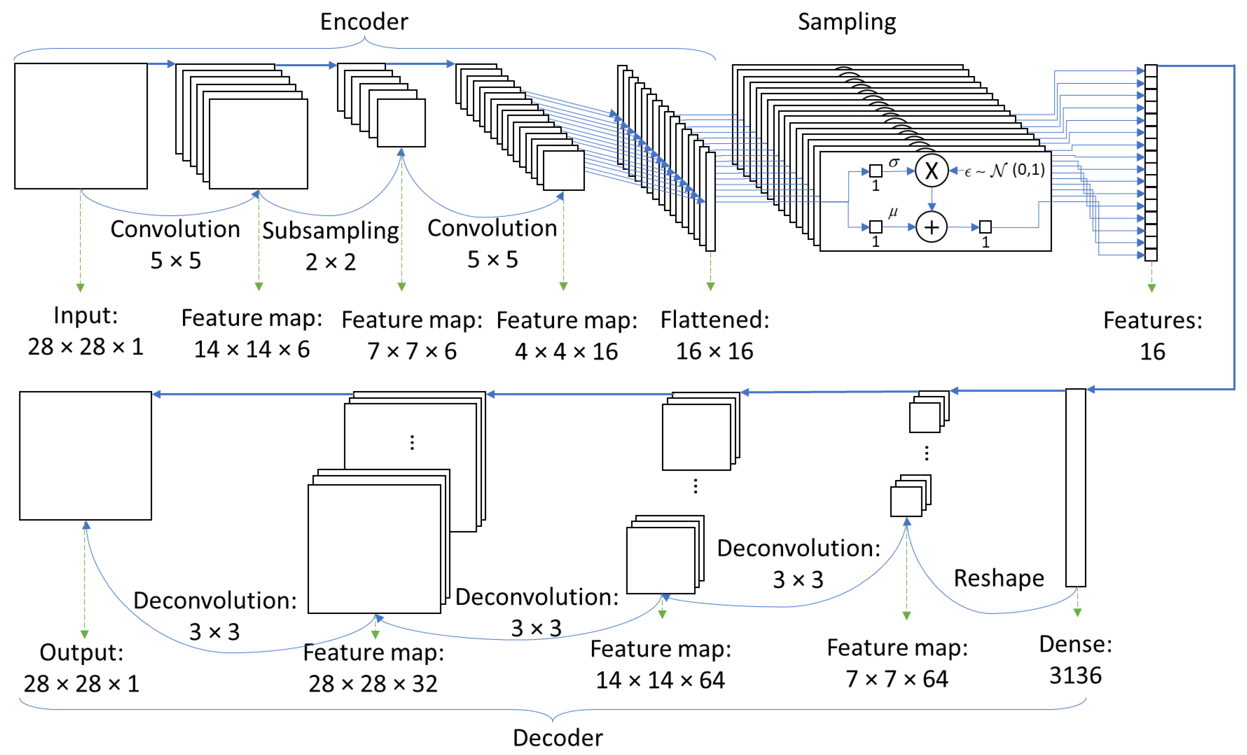
A standard architecture was used as a proof of concept in this work. In particular, a variation of LeNet-5 was employed for the encoder, composed of a convolution layer, followed by a pooling layer which, in turn, was followed by a convolution layer. Each kernel output of this last layer was flattened and fed to the sampling layer. This sampling layer estimates the two parameters of the Gaussian distribution and samples one value which is part of the array that defines the output latent vector. As a result, a Gaussian distribution is produced for each of the last convolution layer’s kernels, and a value is sampled from this distribution.

The decoder output shape should match the encoder input data. Hence, the latent vector fed the decoder’s dense layer (a standard fully connected layer frequently used in feedforward neural networks). The number of neurons used in this dense layer was chosen in a way to avoid the need to use unpooling layers, simplifying the model architecture. The output of this dense layer was then reshaped and fed a sequence of three deconvolutional layers that generated the desired output shape (equal to the encoder input shape).

The implemented VAE architecture is presented in Figure 2. The layer activation function was selected to be the Rectified Linear Unit (ReLU) to improve the network training time. Likewise, during training, the reconstruction loss was the tracked metric, and the model stopped early, with a patient of 5 epochs from the possible 100 epochs, if a minimum improvement of 1 in the tracked metric was not met.

2.3. Kernel Selection Methods

The standard VAE implementation uses one dense layer to learn each parameter of the employed distribution. Hence, two dense layers are usually used since two parameters define the Gaussian distribution. The number of neurons on these layers is the same and defines the latent space. All neurons of the two dense layers are connected to all kernels of the previous convolutional layer, so they all learn distributions from the same feature data.

The proposed approach of this work goes in the opposite direction, using two dense layers (with just one output neuron in each) connected to each kernel from the convolutional layer that provides the features to the distributions. This way, each distribution learns from a single kernel (instead of learning from all kernels), allowing the possibility of assessing which are the most relevant kernels (latent space interpretation) for classification. This can confirm the basic assumption of this work that the sampled features (from each individual kernel) produce dissimilar output distributions (by the sampling layer) for input data from different classes.

Two methodologies were studied to select the most relevant set of latent variables. The first was the benchmark and depended on the classifier, using the standard wrapper SFS method. Particularly, two vectors were produced, one containing all latent variables and a second that was empty. The goal was to create a feature vector to provide the maximum Accuracy (Acc) for the intended classification. In the first iteration, all features of the first vector were used one by one alone, and the most relevant feature (the one that, when used alone, led to the highest Acc) was identified, being moved to the second vector. In the subsequent iterations, the algorithm looked for the features in the first vector that, when combined with the features in the second vector, provide the highest Acc, being sequentially moved to the second vector. This iterative process was repeated until the first vector was empty.

The first methodology is usable when the number of latent variables (denoting the number of kernels) to be evaluated is considerably small since it requires numerous simulations. This problem is addressed by the second methodology proposed in this work, which uses a filter method to assess the relevance of the features. The second method was named KLD selection (KLDS), and its pseudocode is presented in Algorithm 1.

The premise was that a kernel with a lower relevance was more similar to all other kernels; hence, it was less relevant as it conveyed less unique information. Therefore, the created features could be ranked according to the kernel relevance measure, sorting them in a vector from more to less dissimilar (i.e., first was the feature with the highest kernel relevance, then the feature with the second highest kernel relevance, and successively until we reach the feature with the lowest kernel relevance).

The second methodology’s algorithm is composed of three parts: In detail, in the first part of KLDS, several Monte Carlo samples were performed. For each class, the training dataset samples fed the encoder, and the latent space features were stored. As each feature represents one of the kernels in a known sequence, it was then possible to produce the distribution of that kernel for each dataset class. Therefore, number_of_kernels defines the number of distributions (one for each kernel) to be assessed for each dataset class (number_of_classes).

Afterward, for the second part, the distributions assessed for all kernels of one class were examined, calculating for each kernel distribution the KLD between their distribution and the distribution of all other kernels (in pairs). These calculations were then used to determine the mean value of all KLD estimations of each kernel. This process was repeated for all dataset classes, leading to number_of_kernels average KLD estimations (one per kernel), indicated by KLD_measures, for each class. Finally, each kernel’s assessed KLD_measures were averaged (resulting in KLD_kernels) for all classes in the third. The resulting value (for each kernel) was named kernel relevance.

Algorithm 1: Pseudocode for the KLDS algorithm, presenting the required inputs, the produced outputs, and the procedures.

inputs: number_of_classes, number_of_kernels, train_data, train_labels, encoder output: kernel_relevance

for class ← 1 to number_of_classes do

|  samples ← encoder(train_data(train_labels equal to class))

|  kernels_distributions ← distribution(samples)

|  for testing_kernel ← 1 to number_of_kernels do

|  |  for comparing_kernel ← 1 to number_of_kernels do

|  |  |  KLD_measures(testing_kernel, comparing_kernel) ← KLD(testing_kernel, comparing_kernel)

|  |  KLD_kernels(testing_kernel, class) ← mean(KLD_measures(testing_kernel, all))

for testing_kernel ← 1 to number_of_kernels do

|  kernel_relevance(testing_kernel) ← mean(KLD_kernels(testing_kernel, all))

kernel_relevance(testing_kernel) ← sort_descending(kernel_relevance)

The rationale for checking these two methodologies is to verify if a classifier-independent method (the second proposed methodology) can perform similarly to a classifier-dependent method (the first proposed methodology).

Frequently, a classifier-dependent method can produce a better performance but require the selection to be redone when the classifier changes and takes much more time to perform the selection [20]. Hence, when the number of kernels is too high, the classifier-dependent methods become unfeasible, leading to the need for the proposed classifier-independent approach.

2.4. Classification Procedure

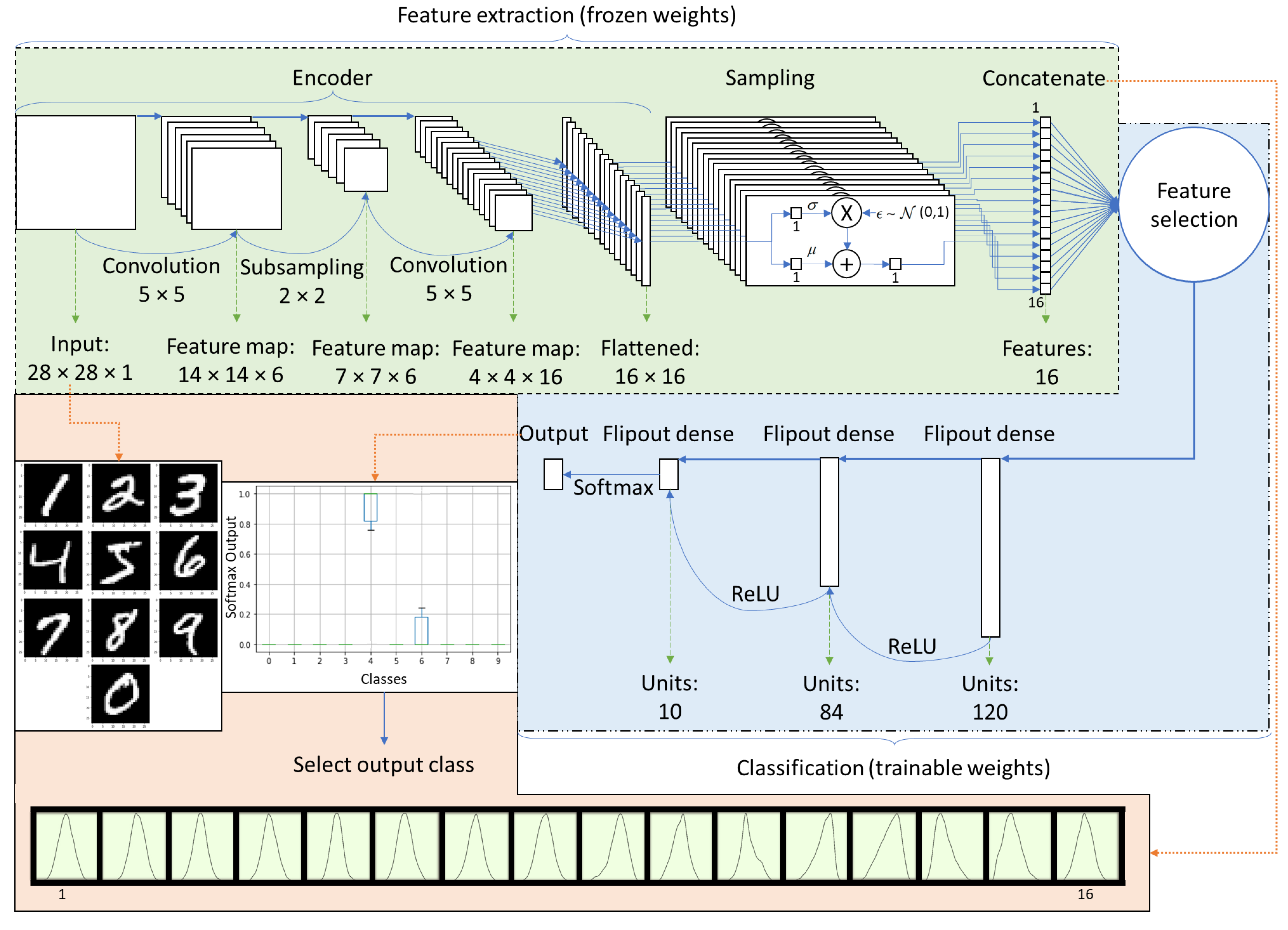
After training the VAE, the encoder was used to produce features, and feature selection was employed to choose the most relevant features to feed a classification procedure.

This classifier, whose structure is presented in Figure 3, was composed of three dense layers following the LeNet-5 architecture. However, these layers were probabilistic to express the uncertainty that arises from inherent data noise and the uncertainty associated with the incompleteness of the model. These two uncertainties are named aleatoric and epistemic, respectively [21].

The probabilistic classifier was developed using Variational Inference (VI) to train the dense layers’ weights while the encoder weights were frozen. These dense layers employ the flipout estimator to decorrelate the gradients within a mini-batch, resolving a central problem associated with VI weight perturbation techniques, where there is a high variance in the gradient estimates as all mini-batch samples share the same perturbation. Therefore, the output of the dense layer forward pass is given by [22]

$$Y=\Phi \left[X\overline{W}+\left[\left(X\circ B\right)\widehat{∆W}\right]\circ A\right],$$

(5)

where $\circ$ is the element-wise multiplication, $\Phi$ is the employed activation function (selected to be ReLU except for the output layer, which used softmax), X are the samples, $\overline{W}$ are the average weights, ${∆W}_s$ is a stochastic perturbation, and two random vectors (A and B) were sampled uniformly from the −1 to 1 range. The VI was also used to solve the ELBO, and the ADAM algorithm was employed to train the model.

2.5. Performance Metrics

The performance of the classifier was assessed using Acc since the standard dataset (MNIST) has a balanced number of samples per class. The main goal is to observe if this metric changes as the number of used features vary. This metric’s 95% Confidence Interval (CI) was also assessed.

The quality of the reconstructed images was also examined as the number of selected features that feeds the decoder varies. For this purpose, the Feature-based SIMilarity index (FSIM) was employed to compare the structural and feature similarity between the restored and original images. This metric is based on the gradient magnitude and phase congruency. The optimal similarity occurs when the FSIM is 1 [23].

3. Results and Discussion

This section first presents the procedure for validating the proposed methodologies and then further discusses the results. This study employed standard publicly available datasets that are well-documented and have been widely utilized for machine-learning and computer vision research. These datasets act as established benchmarks for baseline comparisons, facilitating the evaluation of the proposed methodology against existing state-of-the-art techniques.

The models were examined over multiple runs with random initializations, and similar outcomes were attained in each run. However, it is important to emphasize that each training session for the VAE begins with random weight initialization, potentially resulting in different distributions produced by the samples of the kernel of the last convolution layer of the encoder. Nevertheless, the primary objective of this study is to demonstrate the capacity to reduce the model’s parameter by removing uninformative features while constructing a probabilistic model. To achieve this objective, we show the full process of one run, wherein we train the variational autoencoder through unsupervised learning and, subsequently, as an example, utilize this trained model as a feature generator for a probabilistic classifier (implementing a downstream task of image classification).

3.1. Experimental Procedure

In the first experiment, the model shown in Figure 2 was implemented and provided with data from the MNIST dataset, in which the data provider previously established training and testing datasets. Afterward, the model depicted in Figure 3 was employed to perform the feature-based analysis with a classifier.

During the training of the models, an early-stopping procedure was employed to avoid overfitting, considering 20% of the training dataset as validation and a patience value of 10. The model with all kernels was further examined for the second experiment to perform uncertainty and classification analysis. The last experiment used the model presented in Figure 2. However, the number of features fed to the decoder varied, allowing the FSIM between the input and produced images to be assessed for different settings.

3.2. Kernel Examination and Selection

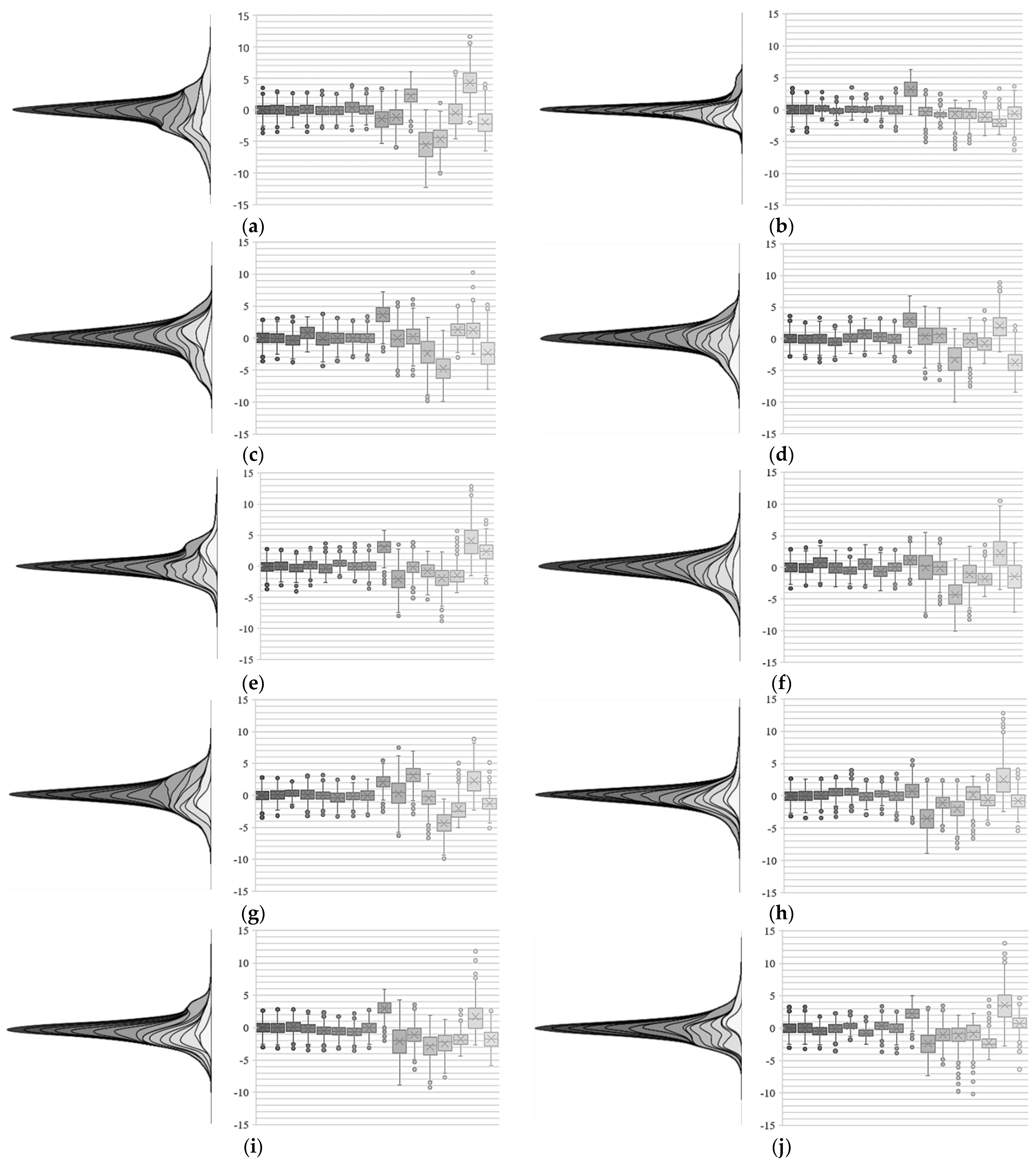
The model presented in Figure 2 was initially trained, and the goal was to evaluate the distribution of the 16 features (produced by the encoder) when only samples of one of the classes (in the test dataset) were presented. These features correspond to the distributions created by evaluating the kernels (one feature per kernel). The boxplots of the samples generated by each feature’s distribution for each dataset class are shown in Figure 4.

By examining Figure 4, it is notorious that several distributions exhibit almost no alteration for all dataset classes, as visible in the eight distributions to the left in Figure 4a–j. This is likely due to the posterior collapse. Therefore, this work hypothesizes that these kernels can be removed from the model, leading to a pruning concept. On the other hand, it is proposed that the kernels that change the most (as visible in the eight distributions to the right in Figure 4a–j) can be the most relevant for a classification task.

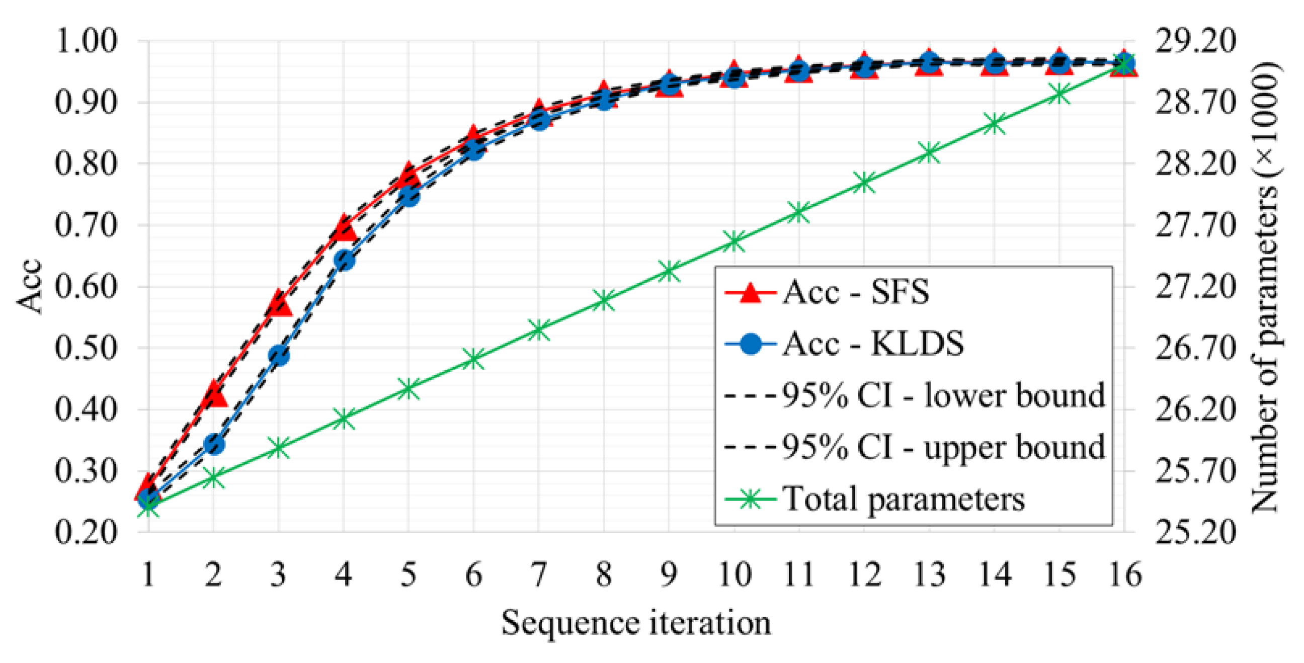
The next step was the creation of the classifier, using the encoder (with frozen weights) as the feature creation layers and training only the probabilistic layers, using the architecture presented in Figure 3. The Acc attained through the iterations of the evaluated feature selection algorithms is shown in Figure 5. It was observed that both algorithms attained a similar performance, choosing the same seven kernels as the least relevant, with an almost identical order. However, the nine most relevant differ in the selected order. Nevertheless, it is possible to observe that the last five selected kernels have a small contribution to the performance improvement, with only a 1% variation.

As a result, the two main hypotheses of this work were confirmed, as the kernels with the lowest alteration in the kernel distributions from the dataset classes were identified as less relevant by both SFS and KLDS. The opposite was true for the kernels’ distributions that varied the most among the dataset classes. However, it is essential to observe that KLDS only required one examination per iteration, leading to 16 examinations. At the same time, SFS made 136 examinations over the 16 iterations. Hence, KLDS only made 12% of the simulations performed by SFS while achieving the same performance, supporting the relevance of this method, especially for models with a large number of kernels to be assessed.

Another relevant aspect is the total number of parameters of the model. As presented in Figure 5, by increasing the number of kernels, the total number of parameters used by the model also increases in a linear progression. Therefore, it is clear that keeping only the most relevant kernels in the classification can help build models with a high relevance for low-computational-resource devices, such as the ones used for IoT.

In this work, if we remove the five least relevant kernels, the total number of parameters of the model is reduced by 4% (1200 parameters) compared to using all 16 kernels. This reduction can be substantial for more complex models that employ millions of parameters.

As an example, using TensorFlow Lite to convert the model (with deterministic layers in the classification) without changing the quantization but removing the five less relevant kernels can lead to a reduction of almost 25 KB in a microcontroller program, a value that can be relevant for resource-constrained devices, where the program will include multiple programming modules in addition to the machine-learning model.

3.3. Uncertainty and Classification Analysis

A relevant aspect of the employed probabilistic classifier is that it can express epistemic and aleatoric uncertainties. Epistemic uncertainty pertains to the inherent uncertainty within the model itself, while aleatoric uncertainty captures the inherent randomness in the data. These two forms of uncertainty are of significant interest in various machine-learning applications, particularly in cases where model reliability and robustness are crucial.

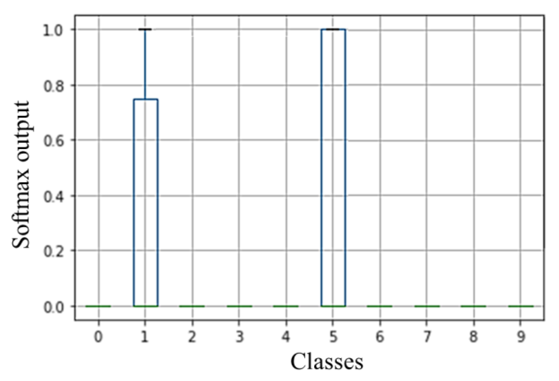
A Monte Carlo sample was used to measure this uncertainty, sampling the forecasts of the model multiple times for each example of the test dataset. An example of the variation in the models’ forecast (the softmax output) from a specific example that was misclassified is presented in Figure 6. This visual representation highlights the challenge of selecting the correct class as the output since both classes 1 and 5 seem to be plausible choices, thereby casting doubt on the reliability of the model’s prediction for this specific instance. It is important to note that this variation in the output is produced by the probabilistic layers of the model, generating a different forecast every time the sample is presented to the already trained model. The higher the variations of the model’s forecasts, the more uncertain the model is about them. This behavior is not present in the trained deterministic models where the output will be the same every time the same sample is fed, thus not showing the model uncertainty.

Furthermore, we conducted a comparative analysis of the probabilistic classifier’s performance against a variant employing deterministic layers instead of probabilistic ones. It was observed that the probabilistic model attained an accuracy (in the test dataset) of 97%, while the performance was 1% lower for the deterministic model. These results suggest that combining probabilistic layers with the VAE’s encoder can result in it better learning the relevant patterns than a deterministic model.

Another important aspect is the performance comparison with a classifier whose encoder was developed using the standard VAE model. This traditional VAE model employs two dense layers to estimate Gaussian distribution parameters, and all distributions are connected to all kernels. The proposed methodology outperformed this standard VAE-based classifier by 2% in terms of average accuracy. This outcome underscores the efficacy and relevance of our proposed methodology in achieving superior classification results.

3.4. Reconstruction Appraisal

To further corroborate the idea that the kernels found to be less relevant (kernels whose distribution varies less among the dataset classes) can be removed, the sequence chosen by KLDS was examined using the FSIM to assess the quality of the reconstructed images. The results of this analysis are presented in Figure 7, which shows the FSIM for all dataset samples. A particular sample was also displayed as an example showing the progress in the reconstruction as the number of used kernels increases (adding the sequence from most to less relevant).

By examining Figure 7, it is possible to conclude that the seven least relevant kernels did not contribute to a relevant improvement in the FSIM, and that, for some samples, an even lower number of kernels could be used (as in the example presented in the figure). These results substantiate the previous analysis.

3.5. Further Validation in Other Datasets

Three more datasets were examined to validate the proposed approach further. These datasets were Fashion-MNIST, Canadian Institute For Advanced Research with ten classes (CIFAR-10), and the Street View House Numbers (SVHN). These datasets were selected since they have ten classes and a similar number of samples, allowing a fair comparison of the results.

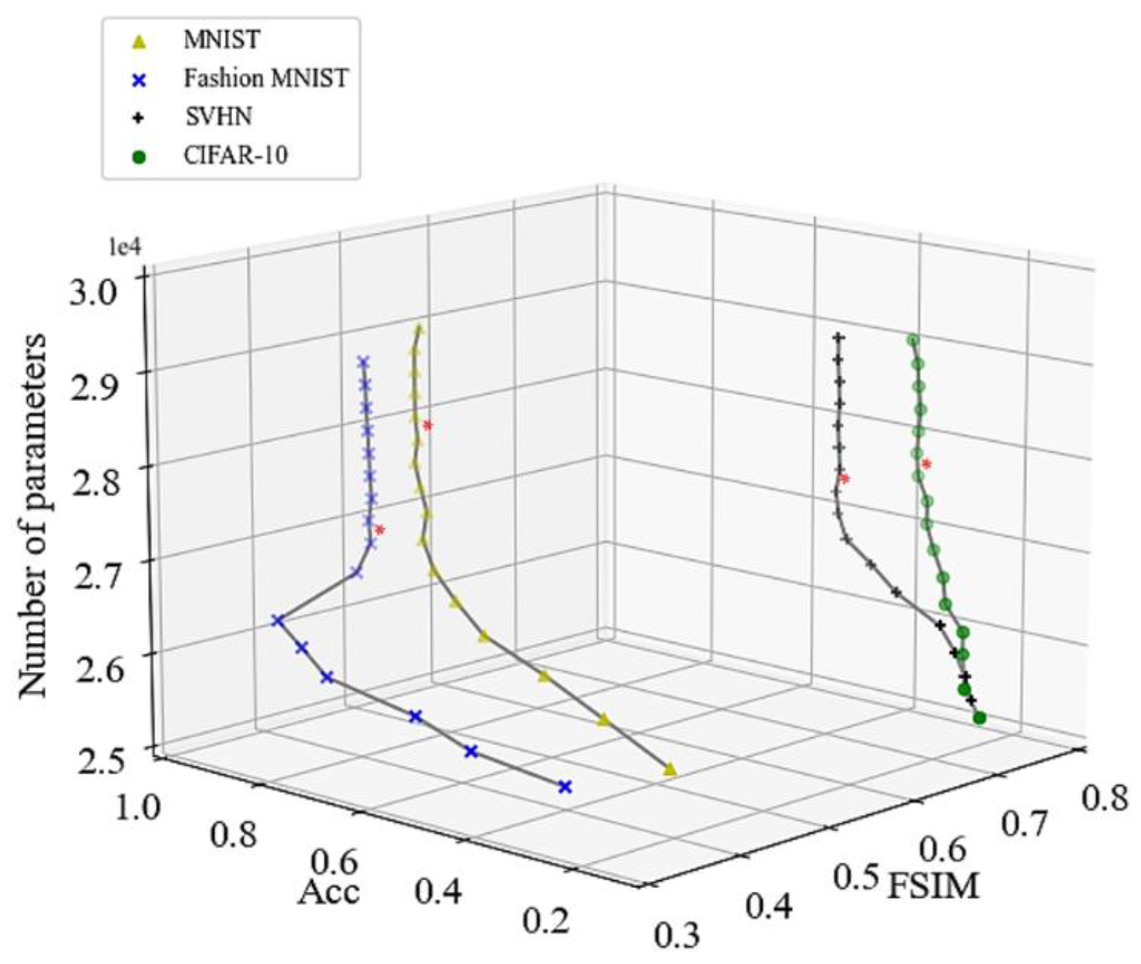
KLDS was used in the three new datasets and selected the relevance of the kernels. Afterward, using the found kernel sequence, and the Acc and FSIM were assessed. The attained results are presented in Figure 8 as the number of parameters of the model (linked to the number of used kernels as shown in Figure 5) increases. The three-channel datasets were converted to a single-channel one.

The asterisk in Figure 8 shows when the increase in the Acc and FSIM becomes irrelevant (less than 1% variation in both metrics). By examining the figure, it is clear that the number of kernels can be reduced in all analyzed datasets without meaningfully affecting the performance, supporting the previous examinations. Specifically, on average, the models used 10 of the 16 kernels in the four examined datasets, denoting a reduction of 37.5%.

4. Conclusions

Kernel selection approaches for classifiers based on the VAE’s encoder are presented in this work, following the rationale of model pruning. The proposed techniques were able to explore the VAE latent space with an interpretation based on the produced kernels’ distributions.

The main hypothesis of this work was confirmed as it was observed that some kernels do not convey relevant information and can be removed. Notably, the proposed KLDS algorithm showed that the kernels with dissimilar distributions are likely the most relevant.

Regarding performance, the examined classifier with probabilistic layers was found to be superior to a model with the same architecture but using deterministic layers. This result is of the utmost relevance as probabilistic models can express epistemic uncertainty, which can be useful in areas such as clinical diagnosis [24].

As a result, the proposed methodology can be used for building applications for resource-constrained devices in multiple IoT areas, such as human activity analysis [25], where there is a need to address the bottleneck in memory usage of the devices to allow the machine-learning models to be implemented on small microcontroller units [26]. Therefore, the next steps of this research should further validate the attained results in real-world data.

Conversely, several main problems are associated with VAEs [2,6], which are also present in this work. Particularly, the sampling procedure will induce noise in the gradients required, and generated data, in the case of images, tend to look blurry with a high probability of looking unrealistic. Furthermore, the usual approach of employing a Gaussian distribution as the prior typically limits the model to learning unimodal representations without allowing dissimilar or mixed data distributions. This work is intended as a proof of concept, employing conventional machine-learning datasets and models. Consequently, it is important to substantiate the proposal through additional experimentation involving diverse model architectures and real-world application datasets.

References

1. Kingma, D.; Welling, M. Auto-encoding variational bayes. In Proceedings of the 2nd International Conference on Learning Representations, ICLR 2014, Banff, AB, Canada, 14–16 April 2014. [Google Scholar]
2. Kingma, D.; Welling, M. An Introduction to Variational Autoencoders. Found. Trends® Mach. Learn. 2019, 12, 307–392. [Google Scholar] [CrossRef]
3. Ternes, L.; Dane, M.; Gross, S.; Labrie, M.; Mills, G.; Gray, J.; Heiser, L.; Chang, Y. A multi-encoder variational autoencoder controls multiple transformational features in single-cell image analysis. Commun. Biol. 2022, 5, 255. [Google Scholar] [CrossRef] [PubMed]
4. Kazeminia, S.; Baur, C.; Kuijper, A.; Ginneken, B.; Navab, N.; Albarqouni, S.; Mukhopadhyay, A. GANs for medical image analysis. Artif. Intell. Med. 2020, 109, 101938. [Google Scholar] [CrossRef] [PubMed]
5. Rezende, D.; Mohamed, S.; Wierstra, D. Stochastic backpropagation and approximate inference in deep generative models. In Proceedings of the 31st International Conference on Machine Learning, Bejing, China, 21–26 June 2014. [Google Scholar]
6. Wei, R.; Garcia, C.; El-Sayed, A.; Peterson, V.; Mahmood, A. Variations in Variational Autoencoders—A Comparative Evaluation. IEEE Access 2020, 8, 153651–153670. [Google Scholar] [CrossRef]
7. Ashiquzzaman, A.; Kim, S.; Lee, D.; Um, T.; Kim, J. Compacting Deep Neural Networks for Light Weight IoT & SCADA Based Applications with Node Pruning. In Proceedings of the 2019 International Conference on Artificial Intelligence in Information and Communication (ICAIIC), Okinawa, Japan, 11–13 January 2019. [Google Scholar]
8. Qi, C.; Shen, S.; Li, R.; Zhao, Z.; Liu, Q.; Liang, J.; Zhang, H. An efficient pruning scheme of deep neural networks for Internet of Things applications. EURASIP J. Adv. Signal Process. 2021, 2021, 31. [Google Scholar] [CrossRef]
9. Singh, A.; Ogunfunmi, T. An Overview of Variational Autoencoders for Source Separation, Finance, and Bio-Signal Applications. Entropy 2022, 24, 55. [Google Scholar] [CrossRef] [PubMed]
10. Yeung, S.; Kannan, A.; Dauphin, Y.; Fei-Fei, L. Tackling Over-pruning in Variational Autoencoders. arXiv 2017. [Google Scholar] [CrossRef]
11. Razavi, A.; Oord, A.v.d.; Poole, B.; Vinyals, O. Preventing Posterior Collapse with delta-VAEs. In Proceedings of the International Conference on Learning Representations, New Orleans, LA, USA, 6–9 May 2019. [Google Scholar]
12. Tomczak, J.; Welling, M. VAE with a VampPrior. In Proceedings of the Twenty-First International Conference on Artificial Intelligence and Statistics, Playa Blanca, Spain, 9–11 April 2018. [Google Scholar]
13. Xu, W.; Tan, Y. Semisupervised Text Classification by Variational Autoencoder. IEEE Trans. Neural Netw. Learn. Syst. 2019, 31, 295–308. [Google Scholar] [CrossRef] [PubMed]
14. Zhao, Q.; Adeli, E.; Honnorat, N.; Leng, T.; Pohl, K.M. Variational AutoEncoder for Regression: Application to Brain Aging Analysis. In Proceedings of the Medical Image Computing and Computer Assisted Intervention—MICCAI 2019, Shenzhen, China, 13–17 October 2019; Shen, D., Liu, T., Peters, T.M., Staib, L.H., Essert, C., Zhou, S., Yap, P.-T., Khan, A., Eds.; Springer International Publishing: Cham, Switzerland, 2019; pp. 823–831. [Google Scholar]
15. Feiyang Cai, A.I.O.; Koutsoukos, X. Variational Autoencoder for Classification and Regression for Out-of-Distribution Detection in Learning-Enabled Cyber-Physical Systems. Appl. Artif. Intell. 2022, 36, 2131056. [Google Scholar] [CrossRef]
16. Lee, S.; Park, S.; Choi, B. Application of domain-adaptive convolutional variational autoencoder for stress-state prediction. Knowl.-Based Syst. 2022, 248, 108827. [Google Scholar] [CrossRef]
17. Blei, D.; Kucukelbir, A.; McAuliffe, J. Variational Inference: A Review for Statisticians. J. Am. Stat. Assoc. 2016, 112, 859–877. [Google Scholar] [CrossRef]
18. Nagi, J.; Ducatelle, F.; Caro, G.; Cireşan, D.; Meier, U.; Giusti, A.; Nagi, F.; Schmidhuber, J.; Gambardella, L. Max-pooling convolutional neural networks for vision-based hand gesture recognition. In Proceedings of the 2011 IEEE International Conference on Signal and Image Processing Applications (ICSIPA), Kuala Lumpur, Malaysia, 16–18 November 2011. [Google Scholar]
19. Noh, H.; Hong, S.; Han, B. Learning deconvolution network for semantic segmentation. In Proceedings of the 2015 IEEE International Conference on Computer Vision (ICCV), Santiago, Chile, 7–13 December 2015. [Google Scholar]
20. Mostafa, S.; Morgado-Dias, F.; Ravelo-García, A. Comparison of SFS and mRMR for oximetry feature selection in obstructive sleep apnea detection. Neural Comput. Appl. 2020, 32, 15711–15731. [Google Scholar] [CrossRef]
21. Ryu, S.; Kwon, Y.; Kim, W. A Bayesian graph convolutional network for reliable prediction of molecular properties with uncertainty quantification. Chem. Sci. 2019, 36, 8438–8446. [Google Scholar] [CrossRef] [PubMed]
22. Wen, Y.; Vicol, P.; Ba, J.; Tran, D.; Grosse, R. Flipout: Efficient Pseudo-Independent Weight Perturbations on Mini-Batches. In Proceedings of the Sixth International Conference on Learning Representations, Vancouver, BC, Canada, 30 April–3 May 2018. [Google Scholar]
23. Zhang, L.; Zhang, L.; Mou, X.; Zhang, D. FSIM: A Feature Similarity Index for Image Quality Assessment. IEEE Trans. Image Process. 2011, 20, 2378–2386. [Google Scholar] [CrossRef] [PubMed]
24. Ozdemir, O.; Russell, R.; Berlin, A. A 3D Probabilistic Deep Learning System for Detection and Diagnosis of Lung Cancer Using Low-Dose CT Scans. IEEE Trans. Med. Imaging 2019, 39, 1419–1429. [Google Scholar] [CrossRef] [PubMed]
25. Amroun, H.; Temkit, M.; Ammi, M. Best Feature for CNN Classification of Human Activity Using IOT Network. In Proceedings of the IEEE/ACM International Conference on and International Conference on Cyber, Physical and Social Computing (CPSCom) Green Computing and Communications (GreenCom) Exeter, Devon, UK, 21–23 June 2017. [Google Scholar]
26. Know, J.; Park, D. Hardware/Software Co-Design for TinyML Voice-Recognition Application on Resource Frugal Edge Devices. Appl. Sci. 2021, 11, 11073. [Google Scholar]
Figure 1. Simplified overview of the proposed methodology, composed of two main steps: The first step develops the VAE, whose encoder was then used for feature creation that fed the classifier created in the second step.
Information 14 00571 g001
Figure 2. Implemented VAE architecture for the two-dimensional input. The layer operations and their produced output shape are also presented.
Information 14 00571 g002
Figure 3. Structure of the classifier used for the classification analysis. The feature extraction part comprises the encoder developed by the VAE, and the weights of this part were frozen (non-trainable). A feature selection procedure was employed for the classification, and the classifier’s weights were optimized using supervised learning.
Information 14 00571 g003
Figure 4. Distributions produced by the samples of the kernel of the last convolution layer of the encoder, for classes (a) 1, (b) 2, (c) 3, (d) 4, (e) 5, (f) 6, (g) 7, (h) 8, (i) 9, and (j) 10, showing the 16 kernels in sequence, from left (kernel 1) to the right (kernel 16). The left figure shows the shape of each distribution produced from the samples, whose amplitude was gradually reduced (from the first to the last kernel) to allow the visualization of all distributions. In contrast, the right figure shows the box plot of the samples.
Information 14 00571 g004
Figure 5. Variation of the Acc through the sequence iteration of the evaluated feature selection algorithms. The total number of parameters of the model, as the number of kernels varies, is also presented.
Information 14 00571 g005
Figure 6. Example of the variation in the models’ forecast (the softmax output) from a specific misclassified sample with high epistemic uncertainty.
Information 14 00571 g006
Figure 7. Variation of the FSIM as the kernels selected by KLDS is progressively used (one by one), from more to less relevant. The image also displays the FSIM variation for a specific example (original image) and the progression in the reconstructed images as the number of used kernels increases.
Information 14 00571 g007
Figure 8. Variation of the Acc and FSIM as the used kernels, whose sequence was selected by KLDS, is progressively increased (leading to an increase in the number of parameters of the model) for the four examined datasets. The asterisk indicates when variation in both metrics is lower than 1%.
Information 14 00571 g008
Disclaimer/Publisher’s Note: The statements, opinions and data contained in all publications are solely those of the individual author(s) and contributor(s) and not of MDPI and/or the editor(s). MDPI and/or the editor(s) disclaim responsibility for any injury to people or property resulting from any ideas, methods, instructions or products referred to in the content.