
ECG-Based Driving Fatigue Detection Using Heart Rate Variability Analysis with Mutual Information


 , ,
, ,  and
and
Abstract
:1. Introduction
- The study did not consider the cognitive fatigue status experienced by drivers when they were fatigued. Several studies [4,5,6] stated that there is an association between driver cognitive fatigue and the causal factor of driving fatigue. Therefore, it is necessary to consider extracting information from interval NN data related to cognitive status.
- The study did not consider the redundant feature factors that can affect the performance of the classification model. It was demonstrated that the Poincare plot analysis and multifractal detrended fluctuation analysis methods only improved in the random forest and AdaBoost models but not in the bagging and gradient boosting models. This is due to the total of 54 features extracted, which makes the model too complex and reduces the model’s interpretability. Therefore, a feature selection method is needed to reduce the number of redundant features.
- In the feature extraction phase, we applied heart rate fragmentation. It was first proposed by Costa et al. [7] and has never been used or further investigated in previous driving fatigue studies (Table 1). Costa et al. [8] reported that heart rate fragmentation can be useful to monitor cognitive status. We hypothesized that heart rate fragmentation can be used to monitor driver cognitive status, which represents the fatigue state of the driver. Heart rate fragmentation is used to extract non-linear features from NN interval data.
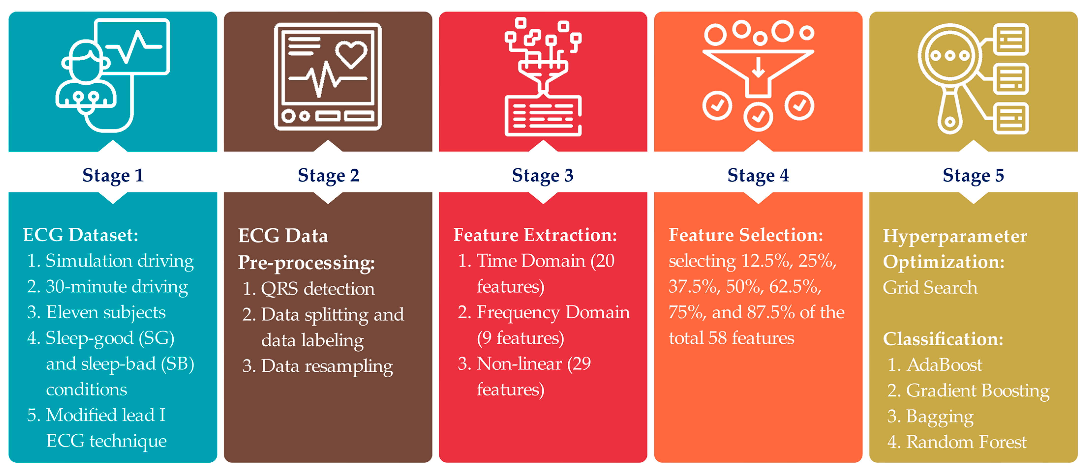
- Our previous study [3] had no feature selection applied in the driving fatigue detection framework; therefore, we added the feature selection phase to the driving fatigue detection framework proposed here (Figure 1). In the feature selection phase, we chose mutual information over other feature selection methods because we applied both linear and non-linear feature extraction methods, and mutual information can capture both linear and non-linear relationships between variables. Additionally, mutual information can be used to measure the relevance of features to the target variable [9].
2. Related Works

| Source (Year) | Number of Subjects | Feature Extraction Method (Number of Features) | Feature Selection | Classification | Class | Accuracy |
|---|---|---|---|---|---|---|
| [24] (2018) | Simulated driving 29 subjects | HRV analysis; time domain (5), freq. domain (5), total: 10 features | Mean decrease accuracy + mean decrease Gini; 6 features selected | KNN | 2 | 75.5% * |
| [20] (2019) | Simulated driving 6 subjects | HRV analysis; weighted standard deviation, weighted mean, dominant respiration, total: 104 features | Greedy feed-forward; 12 features selected | Support Vector Machine | 2 | AUC: 95% * |
| [25] (2019) | Simulated driving 6 subjects | Recurrence plot; non-linear (3) | Convolutional neural network (CNN) | 2 | 70% ** | |
| [21] (2019) | Simulated driving 25 subjects | Wavelet transform; freq. domain (52) | Ensemble logistic regression based on a balanced classification rate value; 24 features selected | 2 | 92.5% *** | |
| [26] (2020) | Simulated driving 10 subjects | HRV analysis; time domain (14), freq. domain (3), non-linear (3), total: 20 features | One-way ANOVA; 15 features selected | Ensemble Learning | 2 | 96.6% *** |
| [23] (2020) | Simulated Driving 27 subjects | HRV analysis; time domain (13), freq. domain (10), non-linear (3), total: 26 features | Correlation-based feature subset selection; 2 features selected | Random Forest | 2 | 97.37% * |
| [27] (2020) | Simulated driving 16 subjects | Cross-correlation and convolution techniques | None | DMKL -SVM | 2 | AUC: 97.1% * |
| [28] (2021) | Real driving 86 subjects | HRV analysis; time domain (8), freq. domain (10), entropy (6), total: 24 features | Sequential forward floating selection (SFFS); 5 features selected | Random Forest | 2 | 85.4% ** |
| [3] (2023) | Simulated driving 11 subjects | HRV analysis; time domain (20), freq. domain (9), non-linear: (25), total: 54 features | None | AdaBoost | 2 | 98.82% * 81.81% ** |
| Random Forest | 2 | 97.98% * 86.36% ** | ||||
3. Materials and Methods
3.1. ECG Dataset
3.2. ECG Data Preprocessing
3.2.1. QRS Detection
3.2.2. Data Splitting and Labeling
3.2.3. Data Resampling
3.3. Feature Extraction
3.3.1. Time Domain Approach
3.3.2. Frequency Domain Approach
3.3.3. Non-Linear Approach
3.4. Feature Selection
3.5. Hyperparameter Optimization and Classification Model
3.5.1. Hyperparameter Optimization
3.5.2. Classification Model
4. Results and Discussion
- 1.
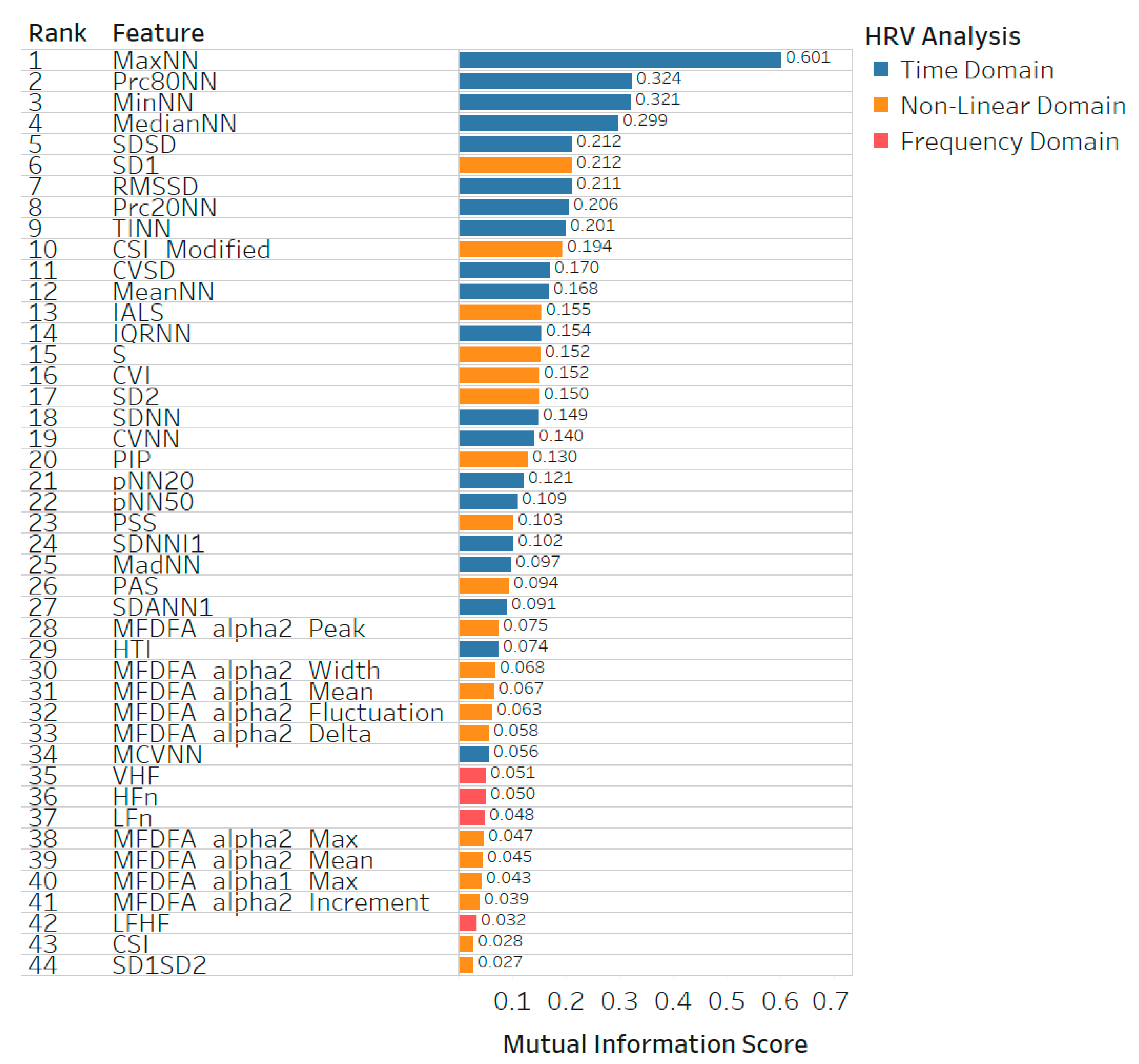
- Conduct a feature ranking of based on the mutual information score between the feature and the target variables. The results of all the mutual information between the feature and the target are ranked from the highest mutual information score to the lowest mutual information score. A higher mutual information score for a feature means that the feature and target variables have a dependency. Thus, the feature represents more useful information for classification [56]. The result of feature ranking is the sequence of features denoted as
- 2.
- Train the model with the number of selected features, from the biggest number of selected features to the smallest number of selected features, and assess the model with the testing dataset. In this paper, we suggest seven experiments, selecting 87.5%, 75%, 62.5%, 50%, 37.5%, 25%, and 12.5% out of all the ranked features ()
- 3.
- Plot the model performance (accuracy) against the number of selected features ( and observe the results. The optimal number of features will be found at the turning point where the highest testing accuracy of a classification model is plotted.
4.1. The Effect of Feature Selection on Model Performance
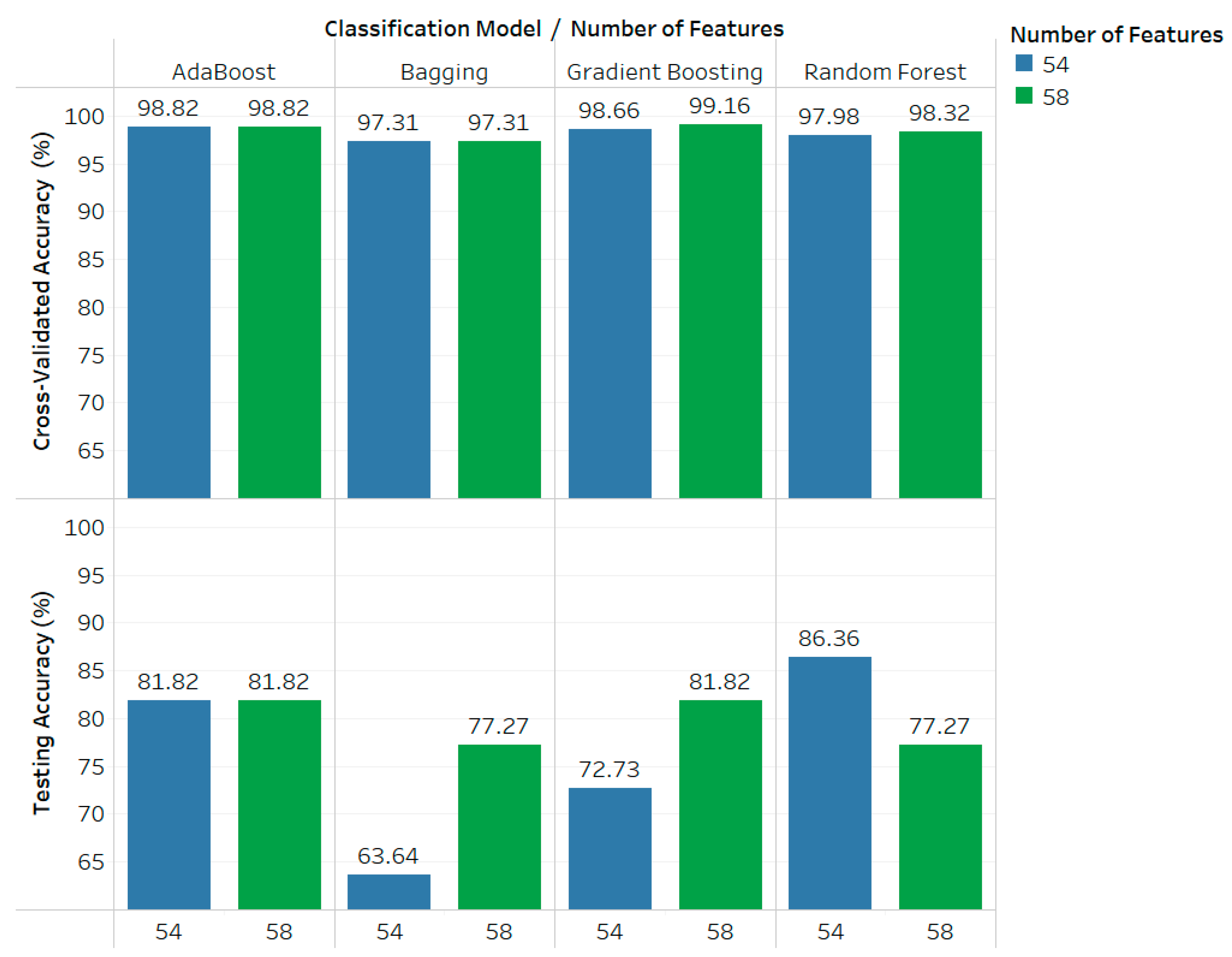
4.1.1. The Performance of Each Classification Model without Feature Selection
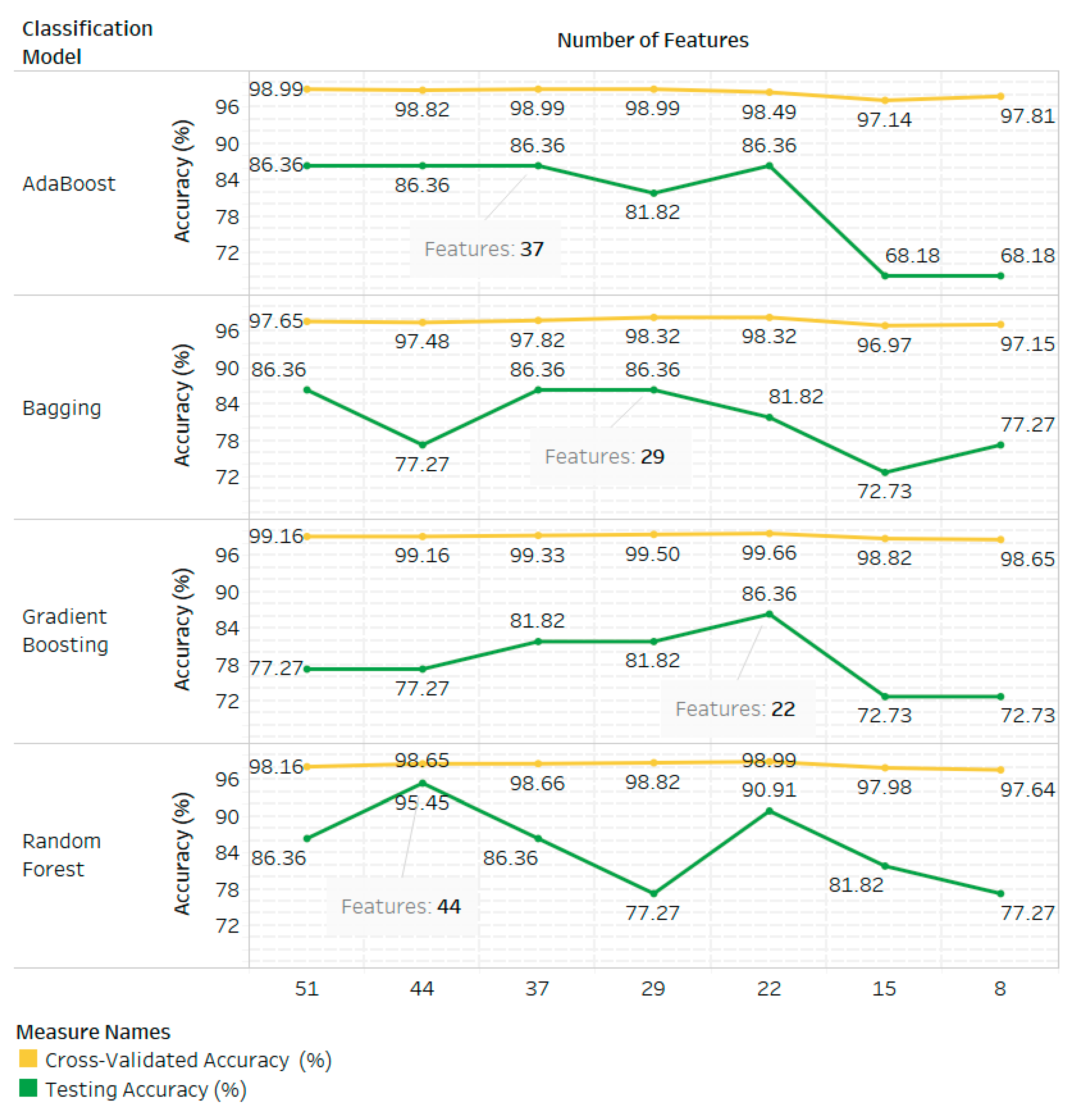
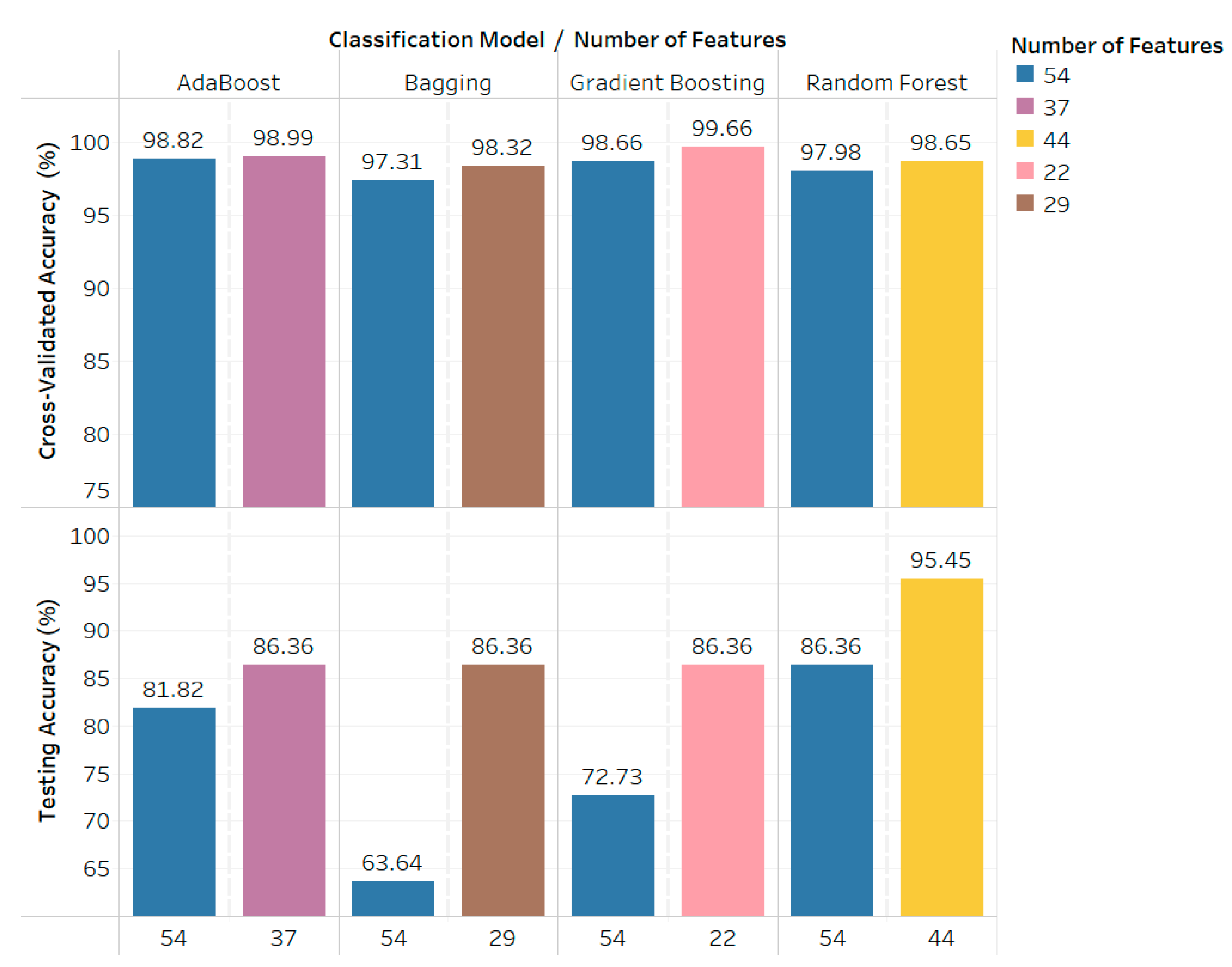
4.1.2. The Performance of Each Classification Model with Feature Selection
4.2. The Necessity of Non-Linear Features in the Proposed Driving Fatigue Framework
4.3. Comparison of the Performance of Each Classification Model in the Proposed Study and the Previous Study and Model Selection
4.4. Future Directions
- Utilizing a co-driver: having a co-driver accompany the main driver during real-world driving can enhance safety by providing assistance and monitoring, thereby minimizing the risk of accidents.
- Driving in monitored and controlled environments: conducting real-world driving scenarios in a controlled and monitored environment can help mitigate accident risks.
- Objective and periodic fatigue assessment: implementing objective and periodic fatigue assessments, overseen by experts in the scientific study of sleep, is crucial to monitoring drivers’ conditions during the experiments.
5. Conclusions
Author Contributions
Funding
Informed Consent Statement
Data Availability Statement
Acknowledgments
Conflicts of Interest
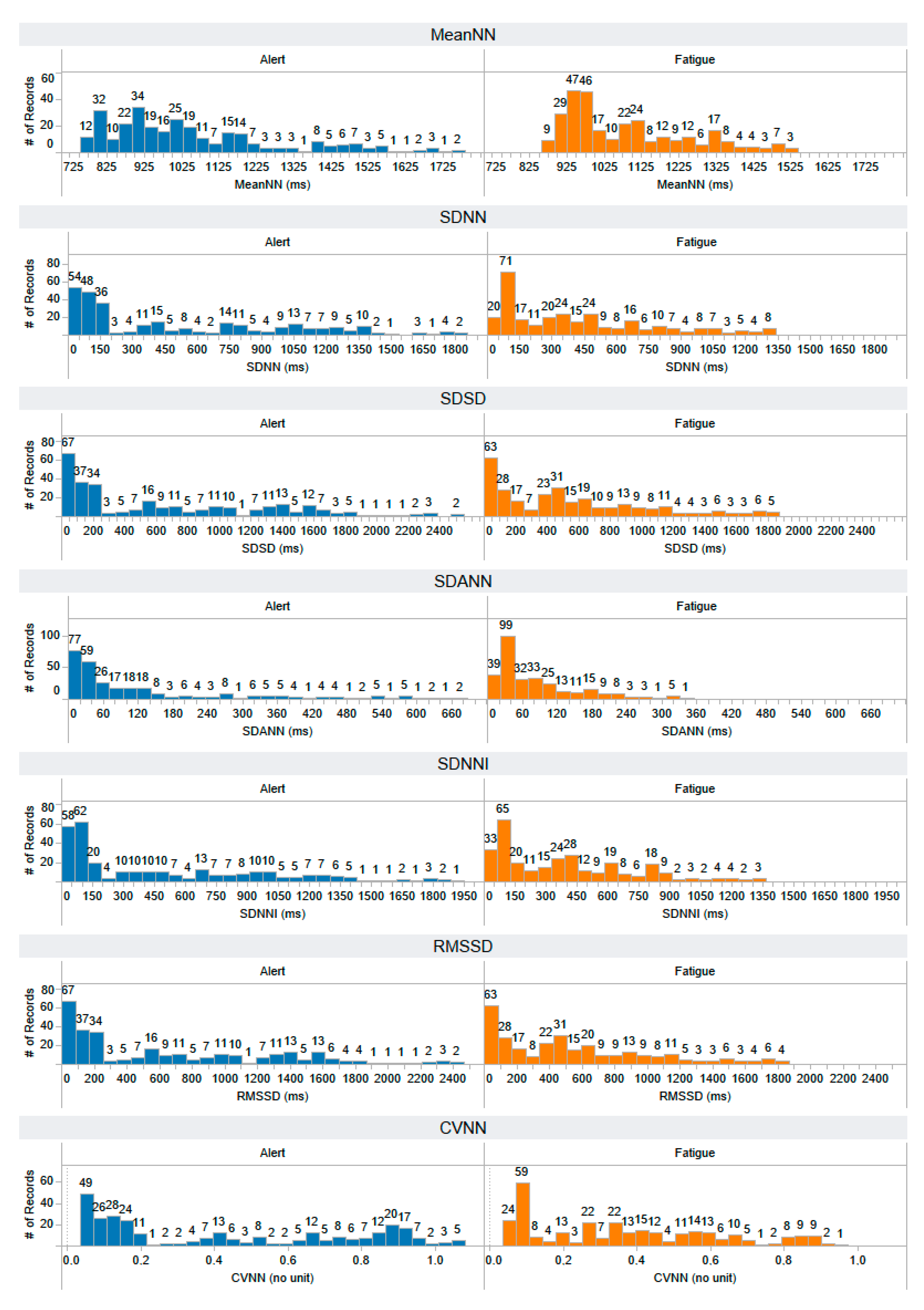
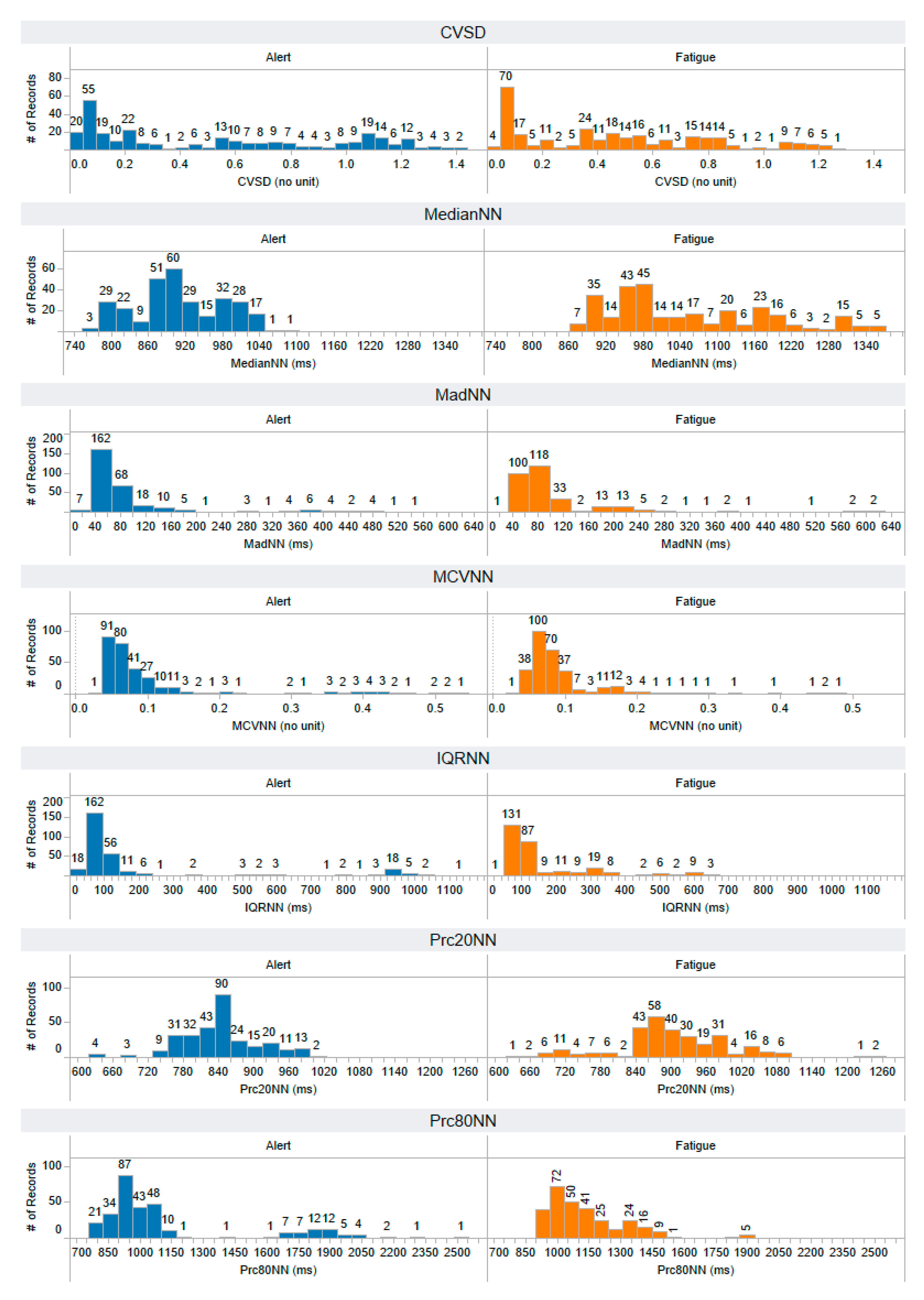
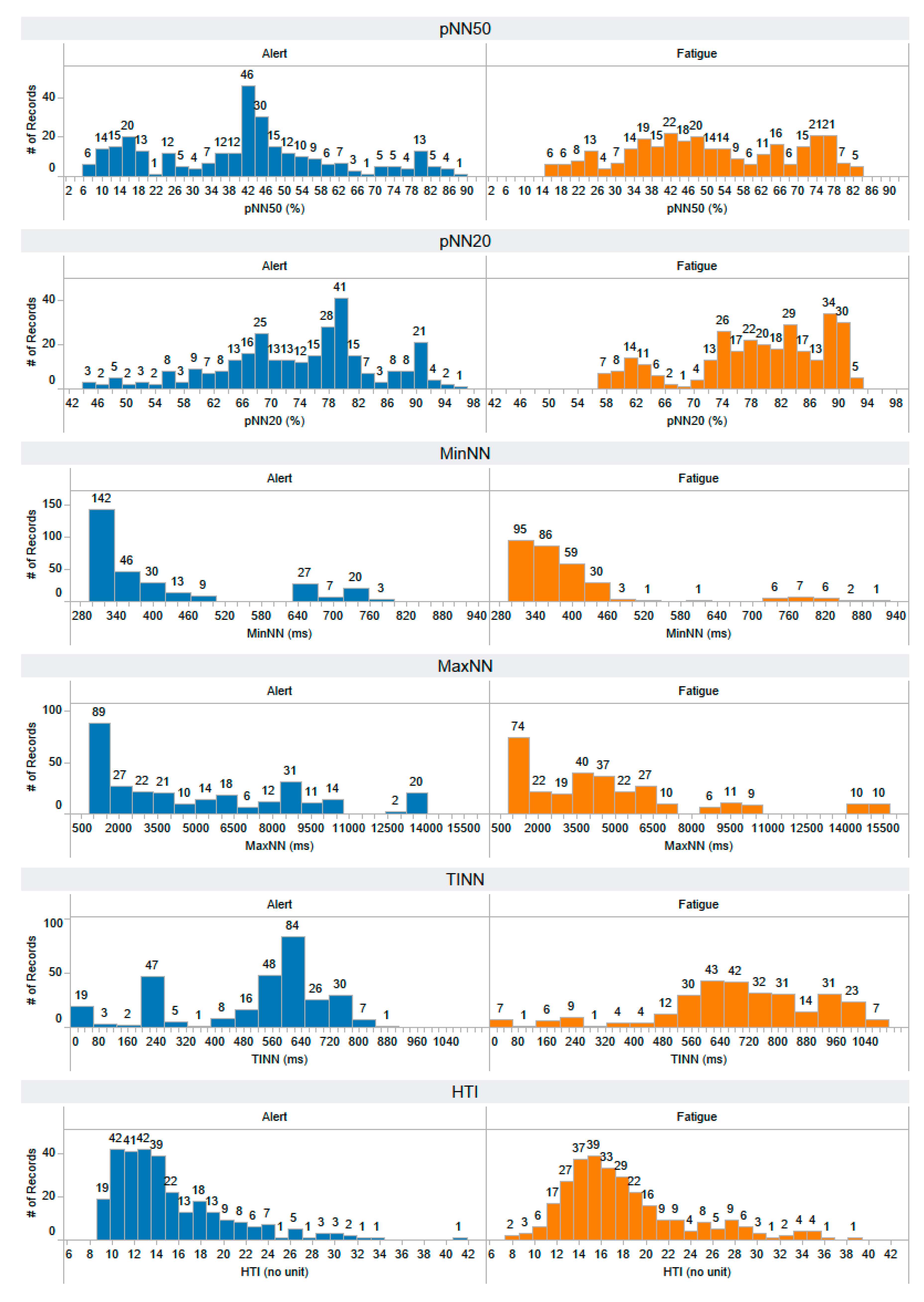
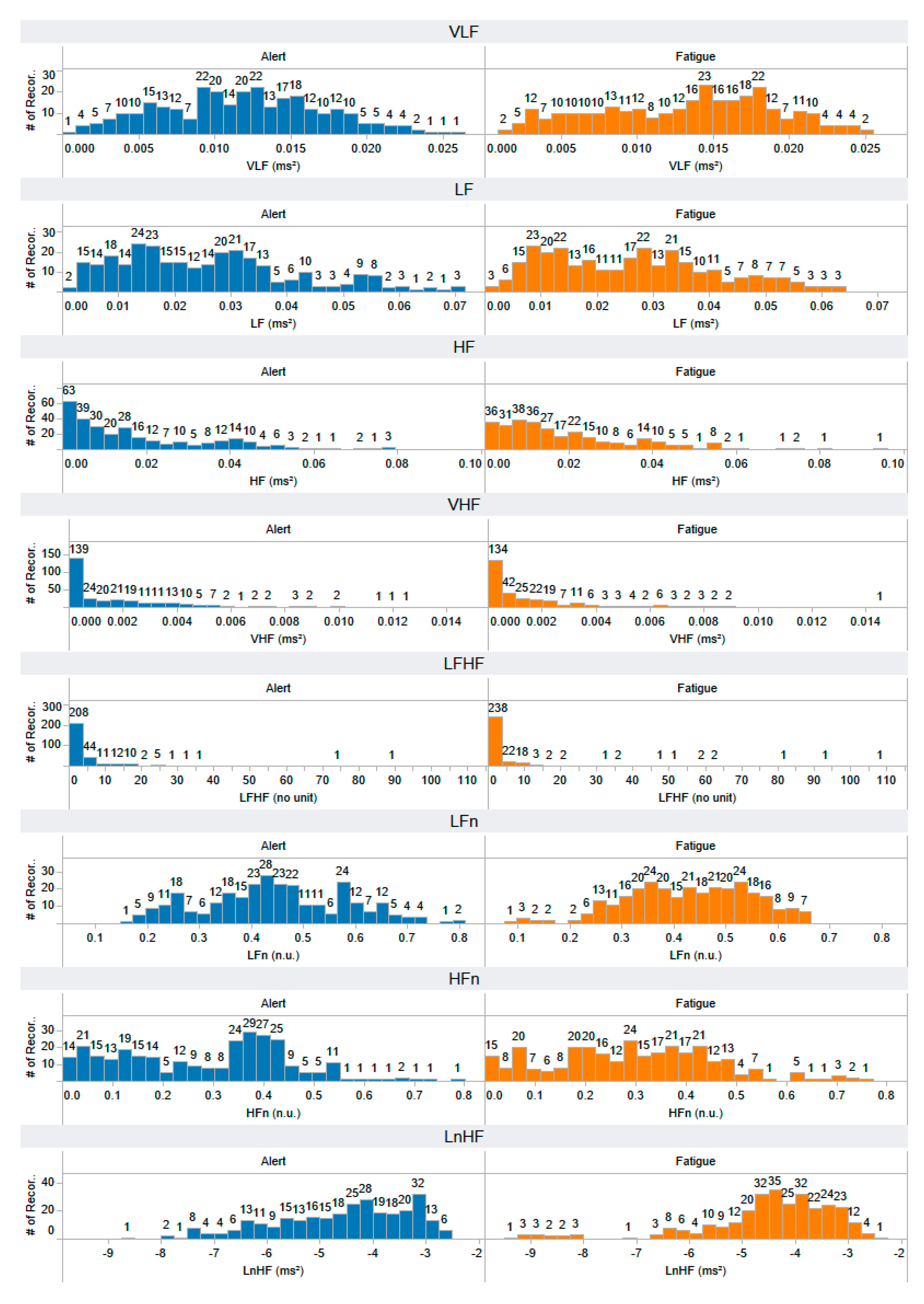
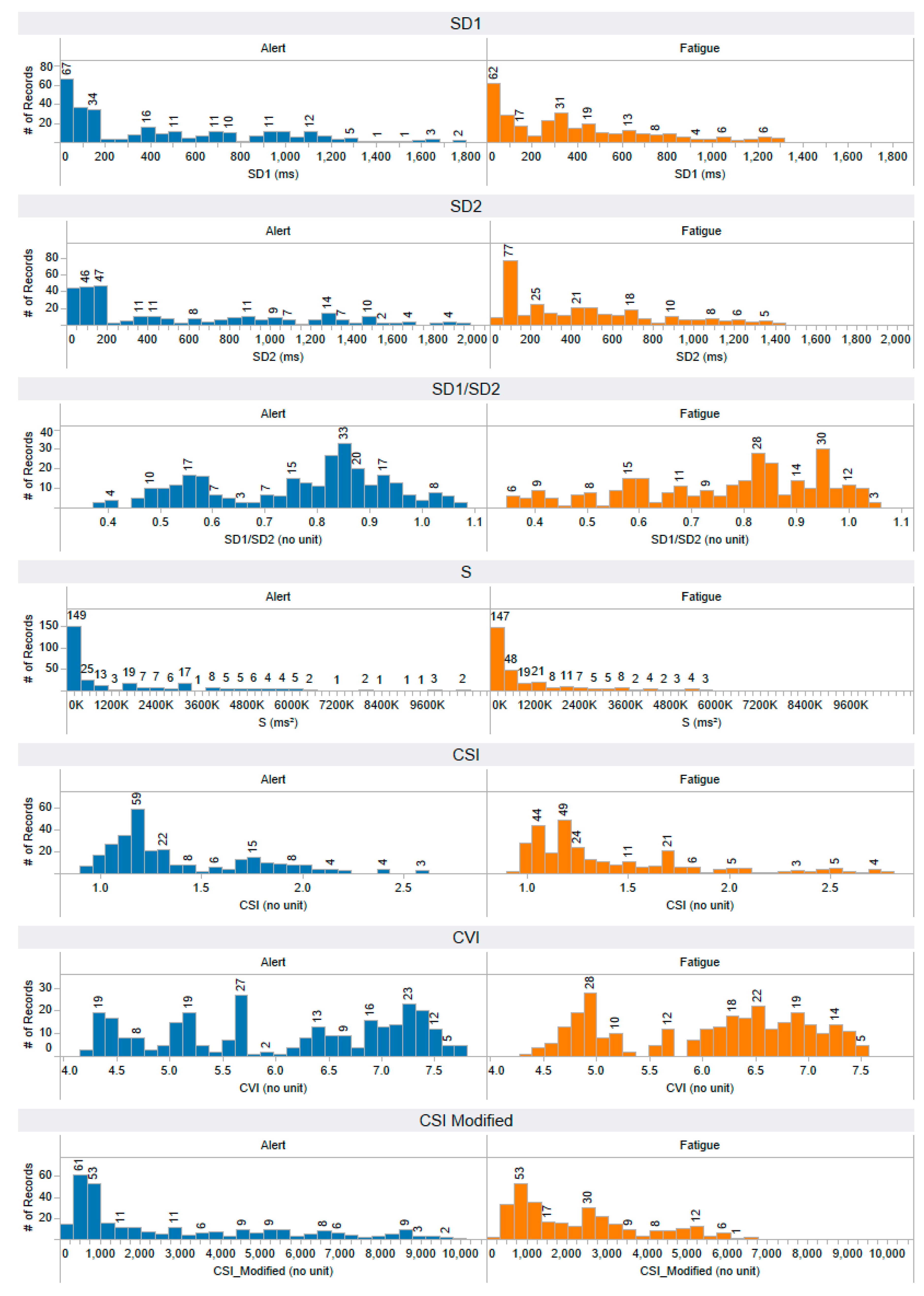
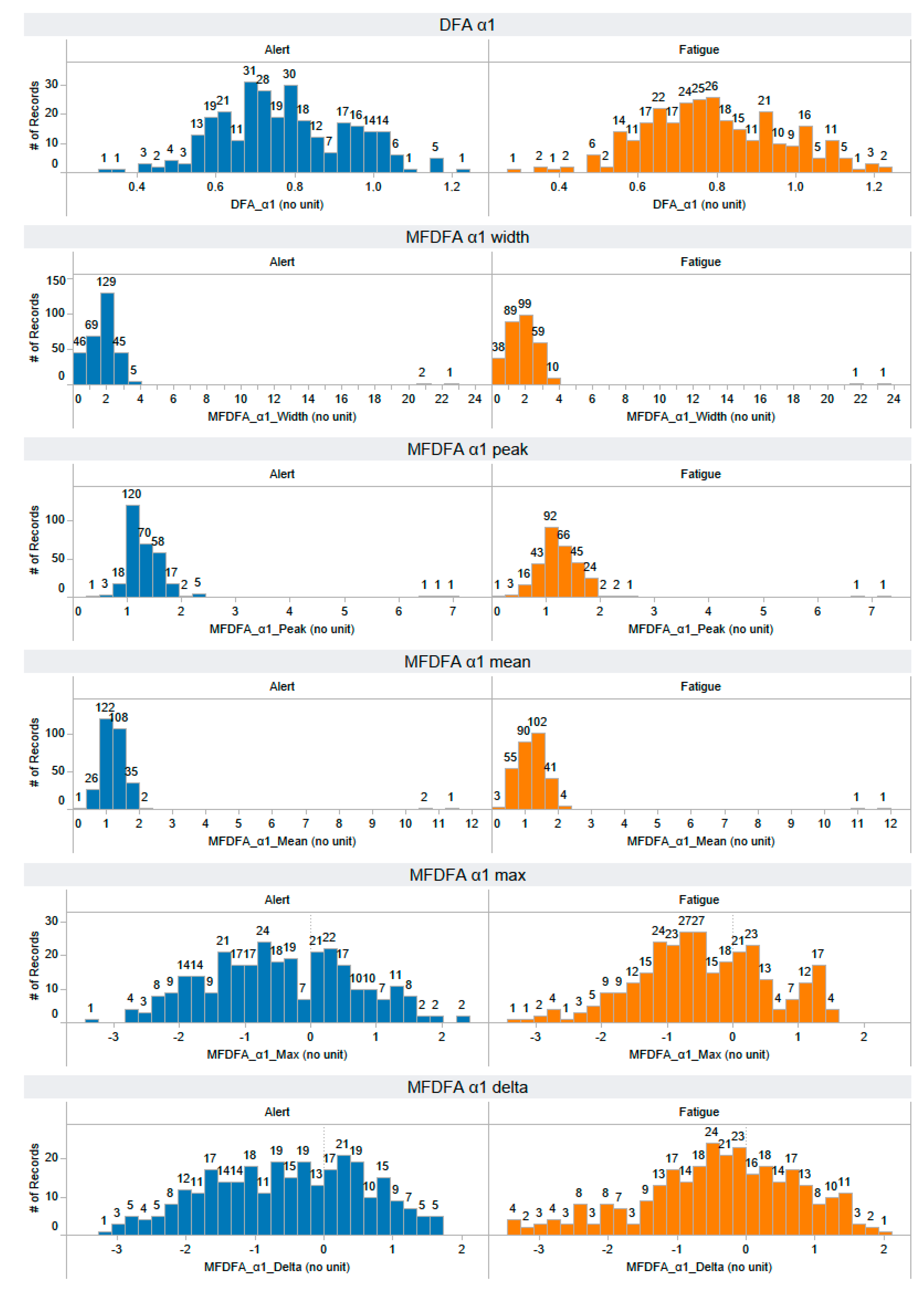
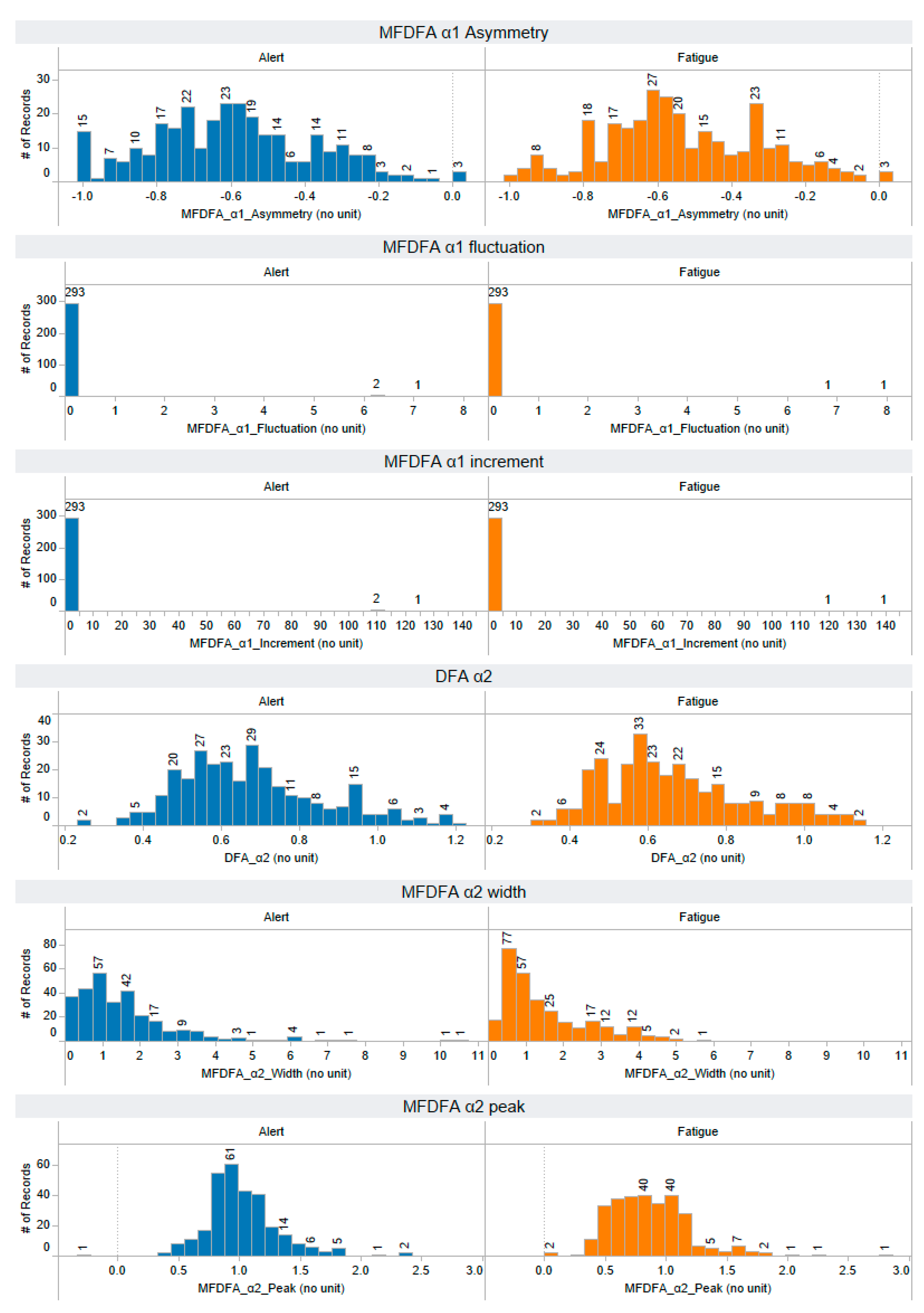
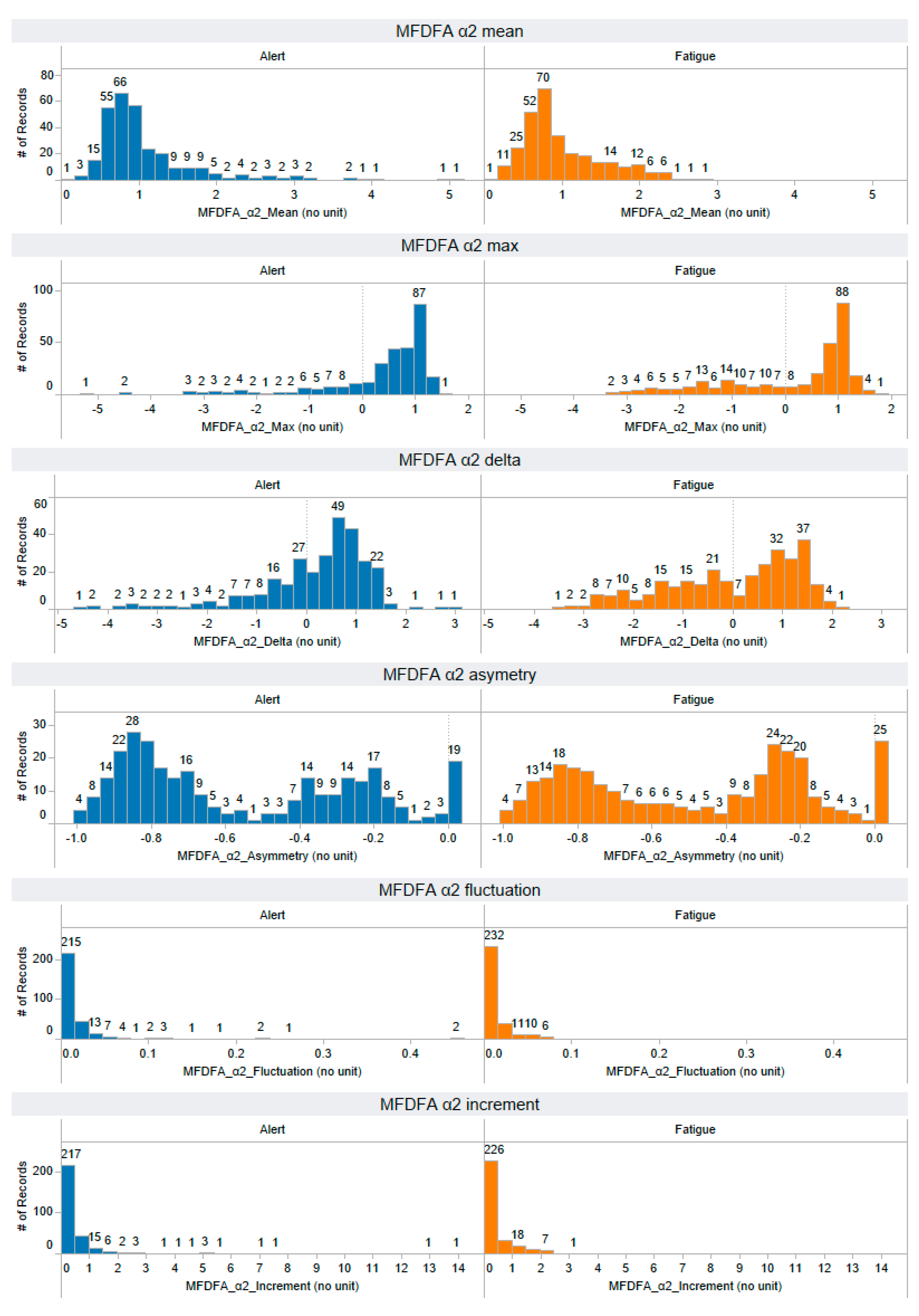
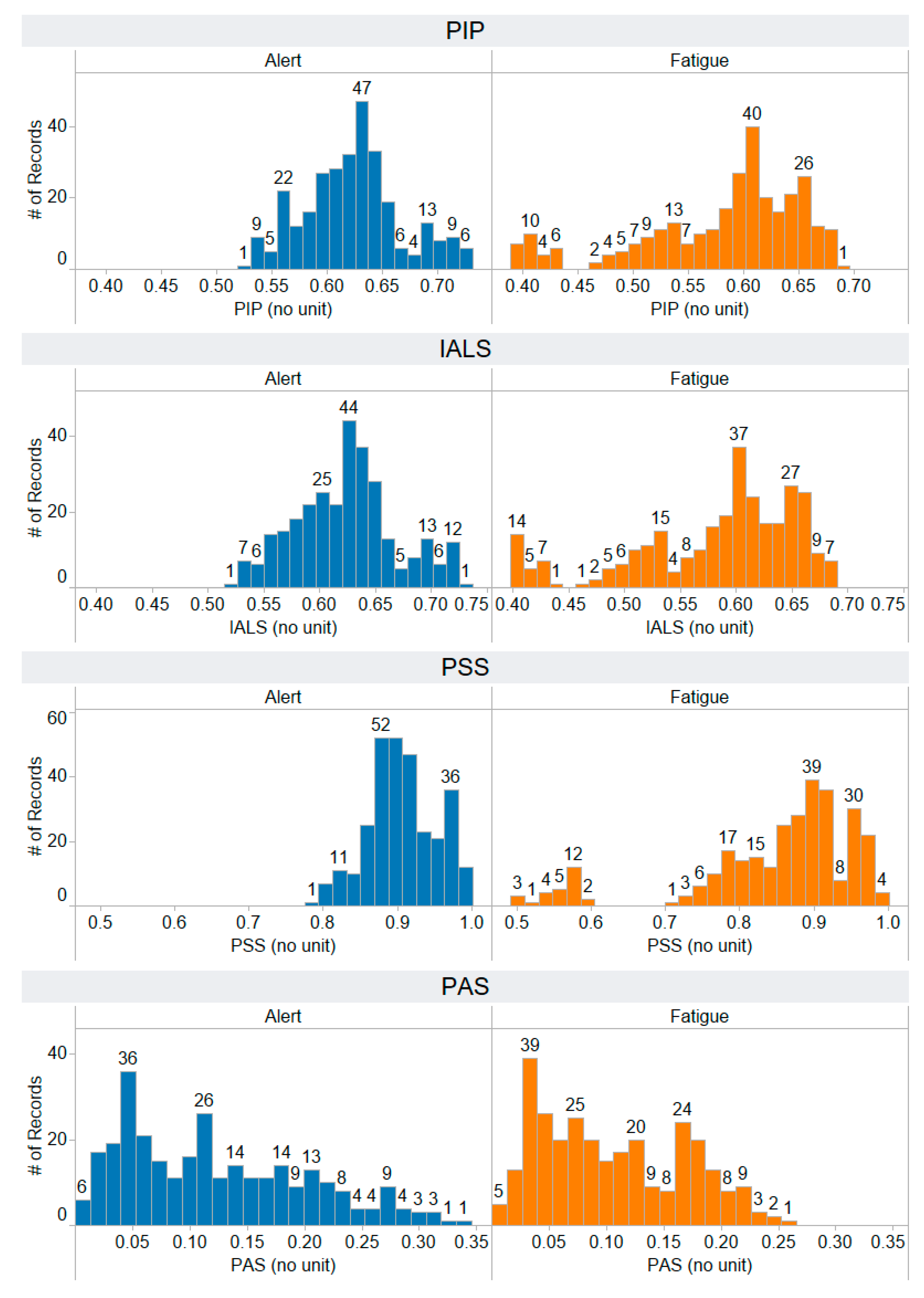
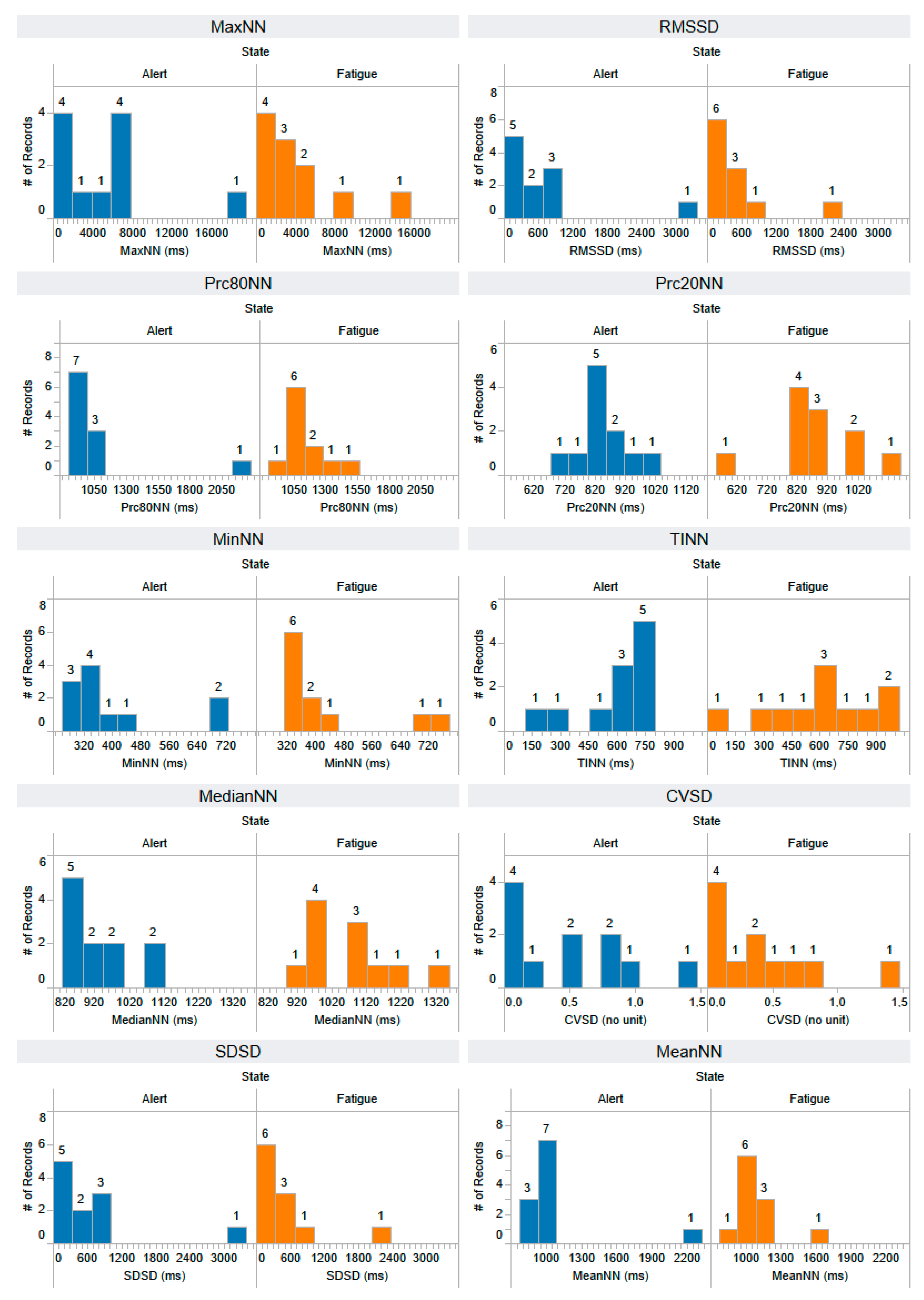
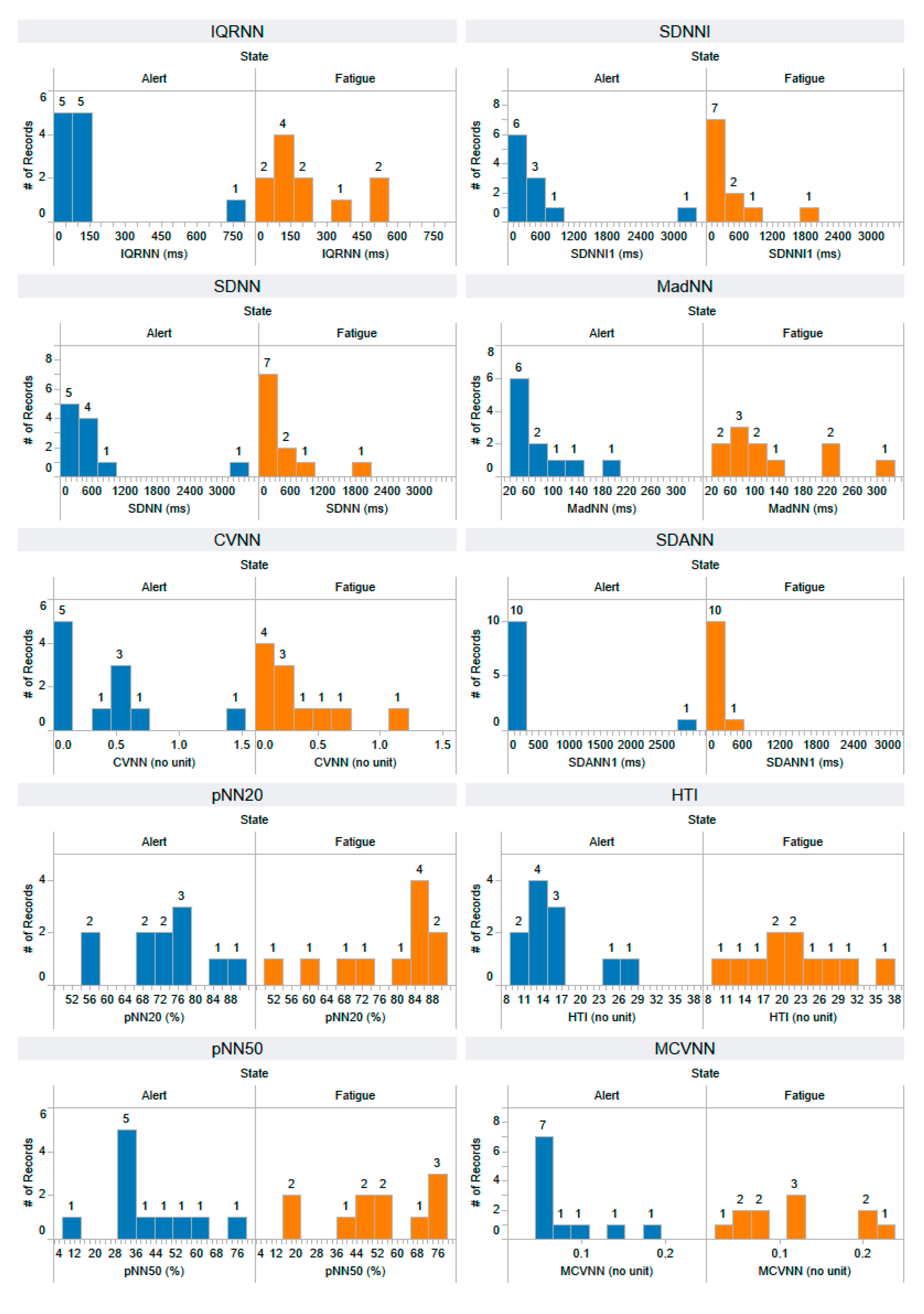
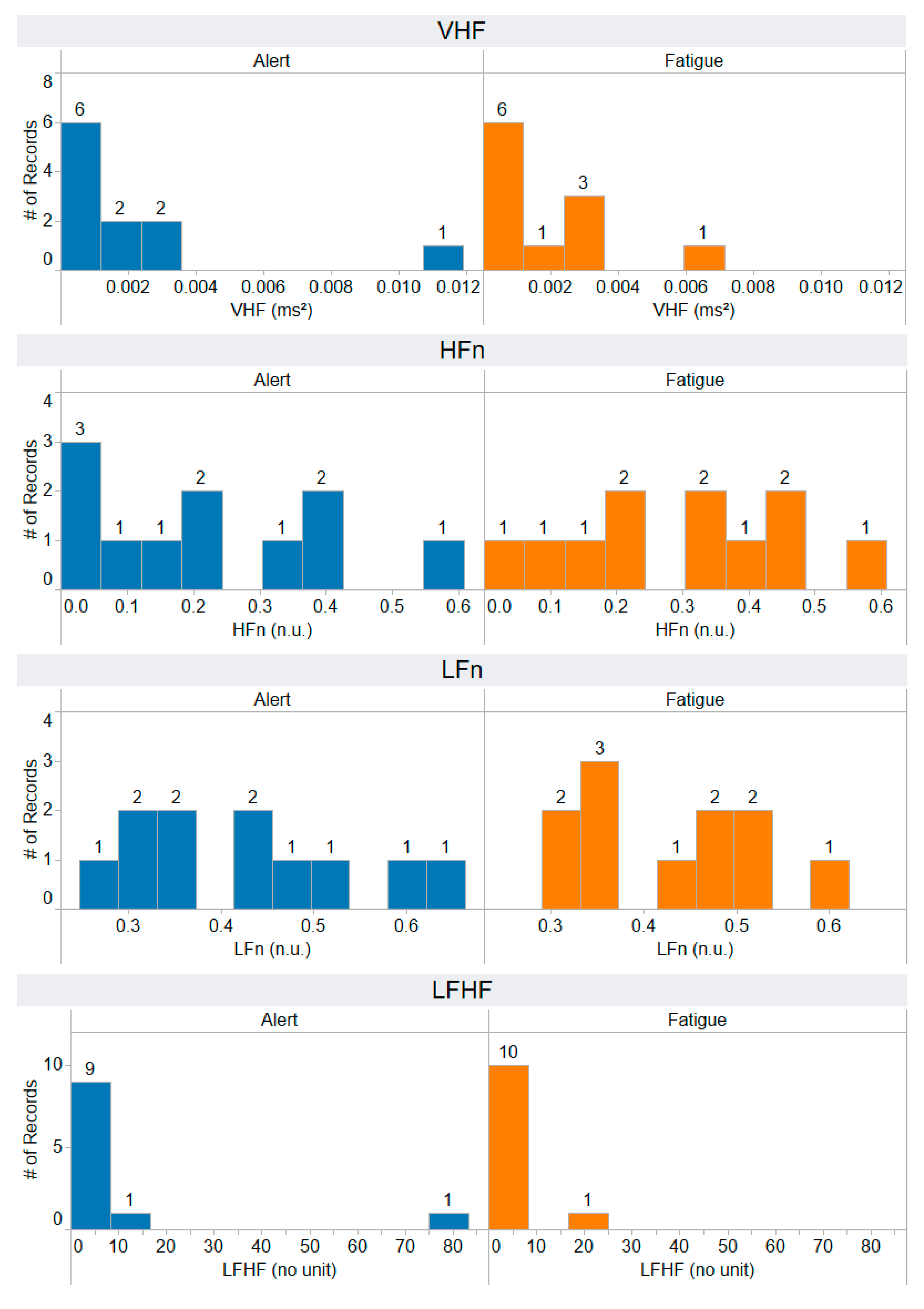
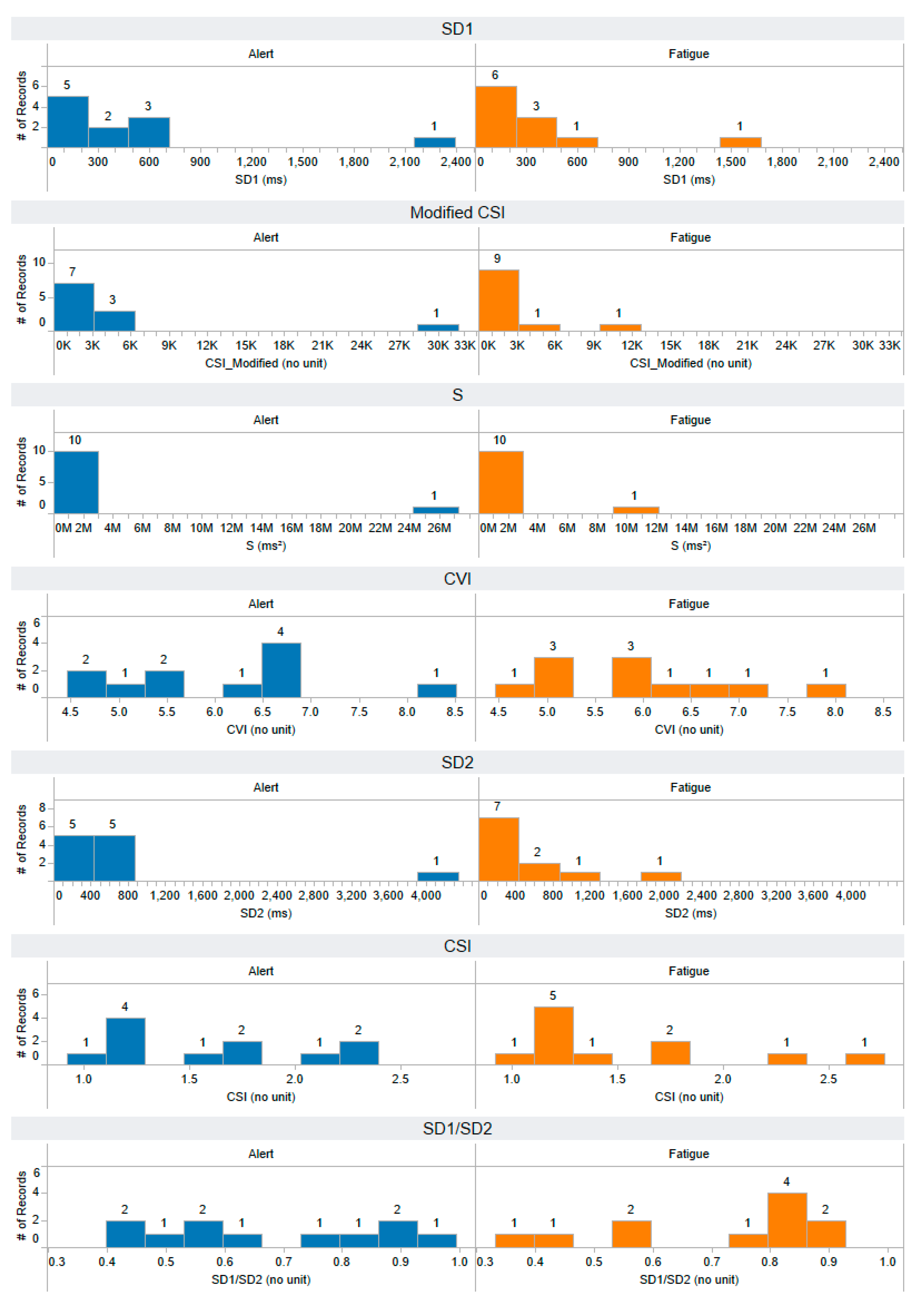
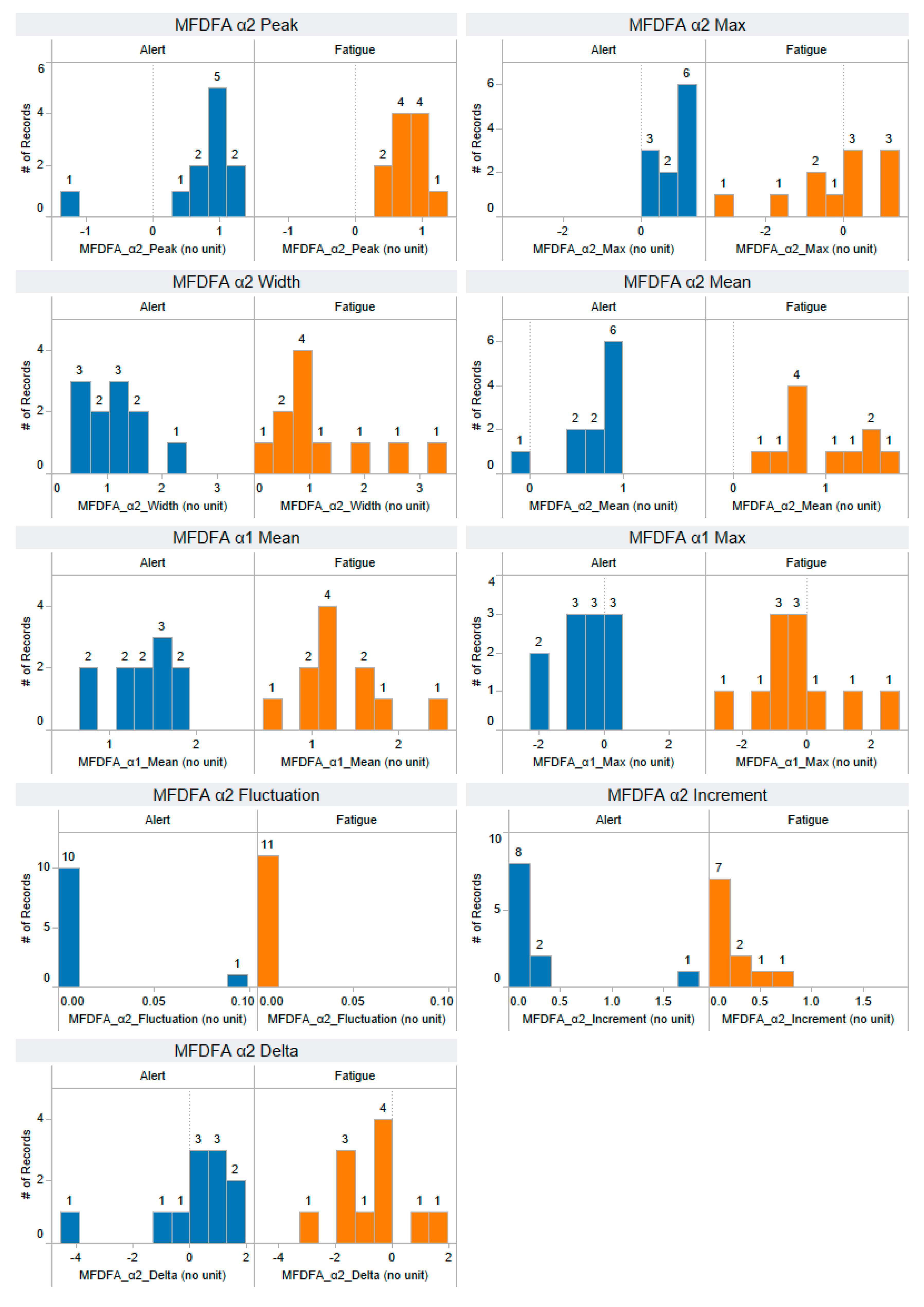
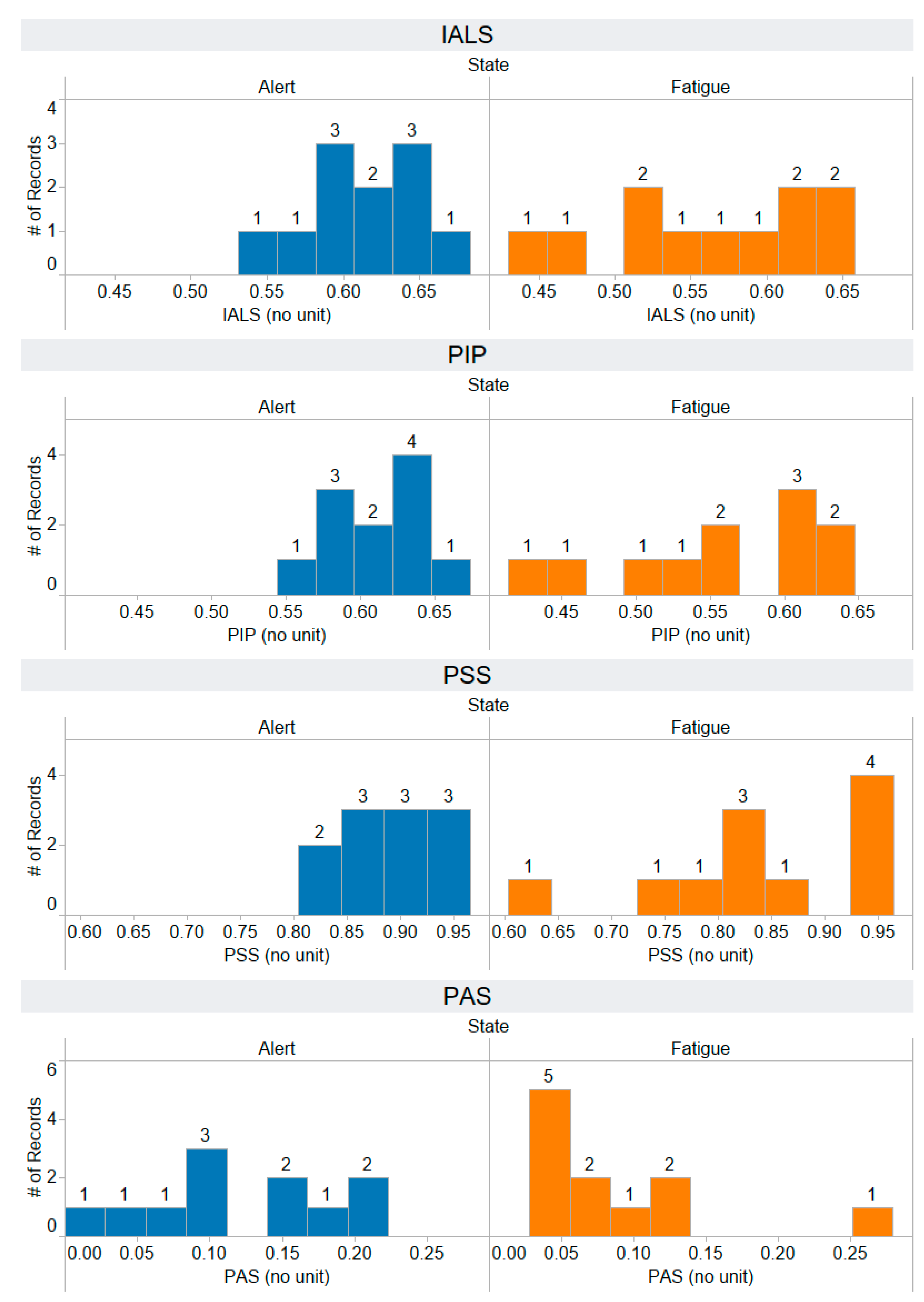
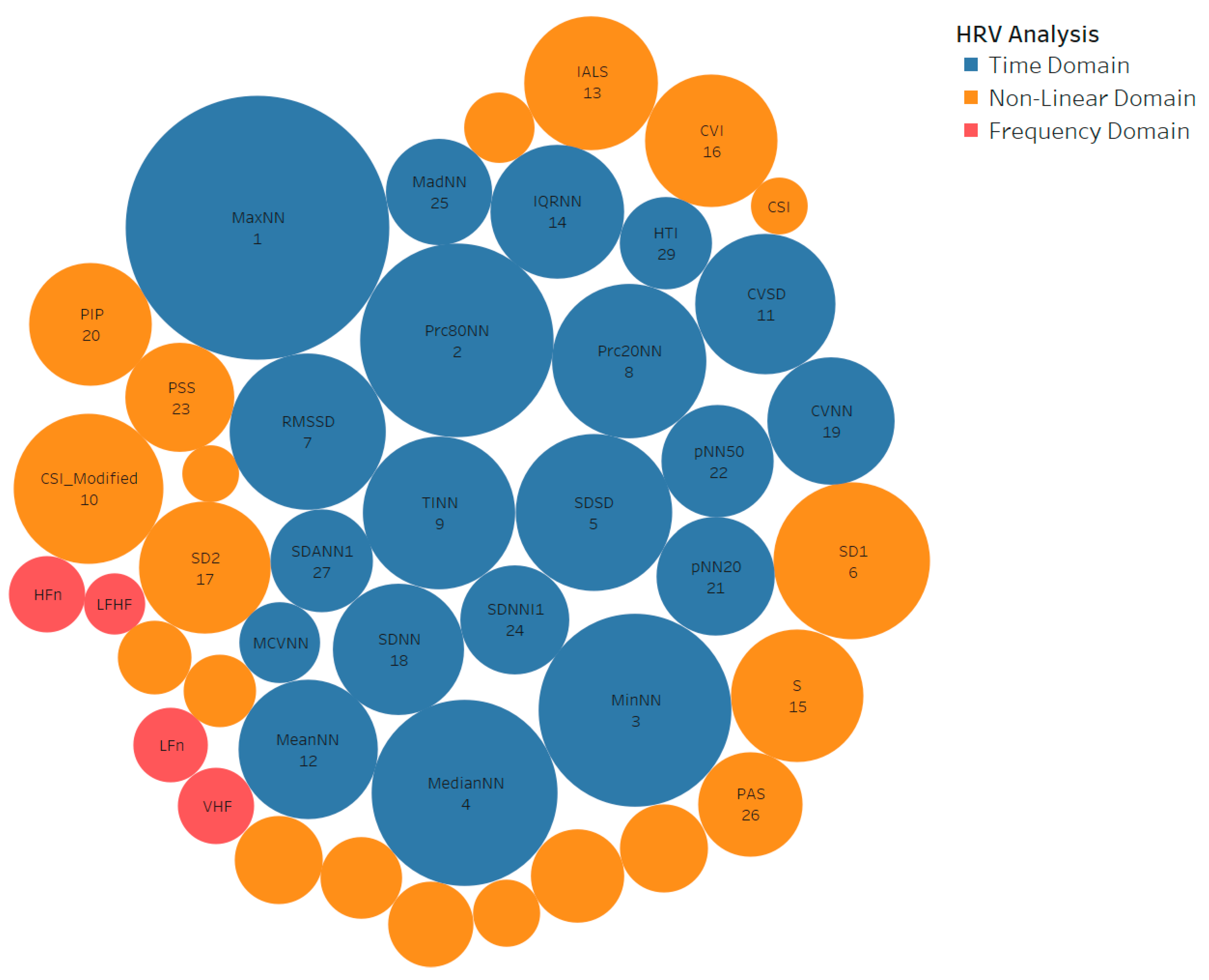
Appendix A. The Distribution of 58 Features Extracted from the Training Dataset
Appendix B. The Distribution of 44 Selected Features Extracted from the Testing Dataset
References
- Mohan, D.; Jha, A.; Chauhan, S.S. Future of road safety and SDG 3.6 goals in six Indian cities. IATSS Res. 2021, 45, 12–18. [Google Scholar] [CrossRef]
- Ani, M.F.; Kamat, S.R.; Fukumi, M.F.; Noh, N.A. A critical review on driver fatigue detection and monitoring system. Int. J. Road Saf. 2020, 1, 53–58. [Google Scholar]
- Halomoan, J.; Ramli, K.; Sudiana, D.; Gunawan, T.S.; Salman, M. A New ECG Data Processing Approach to Developing an Accurate Driving Fatigue Detection Framework with Heart Rate Variability Analysis and Ensemble Learning. Information 2023, 14, 210. [Google Scholar] [CrossRef]
- Ma, J.; Gu, J.; Jia, H.; Yao, Z.; Chang, R. The relationship between drivers’ cognitive fatigue and speed variability during monotonous daytime driving. Front. Psychol. 2018, 9, 459. [Google Scholar] [CrossRef] [PubMed]
- Ansari, S.; Du, H.; Naghdy, F.; Stirling, D. Automatic driver cognitive fatigue detection based on upper body posture variations. Expert Syst. Appl. 2022, 203, 117568. [Google Scholar] [CrossRef]
- Jackson, M.L.; Croft, R.J.; Kennedy, G.; Owens, K.; Howard, M.E. Cognitive components of simulated driving performance: Sleep loss effects and predictors. Accid. Anal. Prev. 2013, 50, 438–444. [Google Scholar] [CrossRef] [PubMed]
- Costa, M.D.; Davis, R.B.; Goldberger, A.L. Heart rate fragmentation: A new approach to the analysis of cardiac interbeat interval dynamics. Front. Physiol. 2017, 8, 255. [Google Scholar] [CrossRef] [PubMed]
- Costa, M.D.; Redline, S.; Hughes, T.M.; Heckbert, S.R.; Goldberger, A.L. Prediction of cognitive decline using heart rate fragmentation analysis: The multi-ethnic study of atherosclerosis. Front. Aging Neurosci. 2021, 13, 708130. [Google Scholar] [CrossRef]
- Song, L.; Langfelder, P.; Horvath, S. Comparison of co-expression measures: Mutual information, correlation, and model based indices. BMC Bioinform. 2012, 13, 328. [Google Scholar] [CrossRef]
- May, J.F.; Baldwin, C.L. Driver fatigue: The importance of identifying causal factors of fatigue when considering detection and countermeasure technologies. Transp. Res. Part F Traffic Psychol. Behav. 2009, 12, 218–224. [Google Scholar] [CrossRef]
- Bier, L.; Wolf, P.; Hilsenbek, H.; Abendroth, B. How to measure monotony-related fatigue? A systematic review of fatigue measurement methods for use on driving tests. Theor. Issues Ergon. Sci. 2020, 21, 22–55. [Google Scholar] [CrossRef]
- Rather, A.A.; Sofi, T.A.; Mukhtar, N. A Survey on Fatigue and Drowsiness Detection Techniques in Driving. In Proceedings of the 2021 International Conference on Computing, Communication, and Intelligent Systems (ICCCIS), Greater Noida, India, 19–20 February 2021; pp. 239–244. [Google Scholar]
- Ramzan, M.; Khan, H.U.; Awan, S.M.; Ismail, A.; Ilyas, M.; Mahmood, A. A survey on state-of-the-art drowsiness detection techniques. IEEE Access 2019, 7, 61904–61919. [Google Scholar] [CrossRef]
- Khunpisuth, O.; Chotchinasri, T.; Koschakosai, V.; Hnoohom, N. Driver drowsiness detection using eye-closeness detection. In Proceedings of the 2016 12th International Conference on Signal-Image Technology & Internet-Based Systems (SITIS), Naples, Italy, 28 November–1 December 2016; pp. 661–668. [Google Scholar]
- Khare, S.K.; Bajaj, V. Entropy-Based Drowsiness Detection Using Adaptive Variational Mode Decomposition. IEEE Sens. J. 2021, 21, 6421–6428. [Google Scholar] [CrossRef]
- Albadawi, Y.; Takruri, M.; Awad, M. A review of recent developments in driver drowsiness detection systems. Sensors 2022, 22, 2069. [Google Scholar] [CrossRef] [PubMed]
- Sikander, G.; Anwar, S. Driver fatigue detection systems: A review. IEEE Trans. Intell. Transp. Syst. 2018, 20, 2339–2352. [Google Scholar] [CrossRef]
- Gao, X.-Y.; Zhang, Y.-F.; Zheng, W.-L.; Lu, B.-L. Evaluating driving fatigue detection algorithms using eye tracking glasses. In Proceedings of the 2015 7th International IEEE/EMBS Conference on Neural Engineering (NER), Montpellier, France, 22–24 April 2015; pp. 767–770. [Google Scholar]
- Soler, A.; Moctezuma, L.A.; Giraldo, E.; Molinas, M. Automated methodology for optimal selection of minimum electrode subsets for accurate EEG source estimation based on Genetic Algorithm optimization. Sci. Rep. 2022, 12, 11221. [Google Scholar] [CrossRef] [PubMed]
- Kim, J.; Shin, M. Utilizing HRV-derived respiration measures for driver drowsiness detection. Electronics 2019, 8, 669. [Google Scholar] [CrossRef]
- Babaeian, M.; Amal Francis, K.; Dajani, K.; Mozumdar, M. Real-time driver drowsiness detection using wavelet transform and ensemble logistic regression. Int. J. Intell. Transp. Syst. Res. 2019, 17, 212–222. [Google Scholar] [CrossRef]
- Khalid, S.; Khalil, T.; Nasreen, S. A survey of feature selection and feature extraction techniques in machine learning. In Proceedings of the 2014 Science and Information Conference, London, UK, 27–29 August 2014; pp. 372–378. [Google Scholar]
- Kundinger, T.; Sofra, N.; Riener, A. Assessment of the potential of wrist-worn wearable sensors for driver drowsiness detection. Sensors 2020, 20, 1029. [Google Scholar] [CrossRef]
- Huang, S.; Li, J.; Zhang, P.; Zhang, W. Detection of mental fatigue state with wearable ECG devices. Int. J. Med. Inform. 2018, 119, 39–46. [Google Scholar] [CrossRef]
- Lee, H.; Lee, J.; Shin, M. Using wearable ECG/PPG sensors for driver drowsiness detection based on distinguishable pattern of recurrence plots. Electronics 2019, 8, 192. [Google Scholar] [CrossRef]
- Murugan, S.; Selvaraj, J.; Sahayadhas, A. Detection and analysis: Driver state with electrocardiogram (ECG). Phys. Eng. Sci. Med. 2020, 43, 525–537. [Google Scholar] [CrossRef] [PubMed]
- Chui, K.T.; Lytras, M.D.; Liu, R.W. A generic design of driver drowsiness and stress recognition using MOGA optimized deep MKL-SVM. Sensors 2020, 20, 1474. [Google Scholar] [CrossRef] [PubMed]
- Persson, A.; Jonasson, H.; Fredriksson, I.; Wiklund, U.; Ahlström, C. Heart rate variability for classification of alert versus sleep deprived drivers in real road driving conditions. IEEE Trans. Intell. Transp. Syst. 2020, 22, 3316–3325. [Google Scholar] [CrossRef]
- Ahn, S.; Nguyen, T.; Jang, H.; Kim, J.G.; Jun, S.C. Exploring neuro-physiological correlates of drivers’ mental fatigue caused by sleep deprivation using simultaneous EEG, ECG, and fNIRS data. Front. Hum. Neurosci. 2016, 10, 219. [Google Scholar] [CrossRef] [PubMed]
- Oweis, R.J.; Al-Tabbaa, B.O. QRS detection and heart rate variability analysis: A survey. Biomed. Sci. Eng. 2014, 2, 13–34. [Google Scholar]
- Pan, J.; Tompkins, W.J. A real-time QRS detection algorithm. IEEE Trans. Biomed. Eng. 1985, 32, 230–236. [Google Scholar] [CrossRef] [PubMed]
- Cui, Y.; Jia, M.; Lin, T.-Y.; Song, Y.; Belongie, S. Class-balanced loss based on effective number of samples. In Proceedings of the IEEE/CVF Conference on Computer Vision and Pattern Recognition, Long Beach, CA, USA, 15–20 June 2019; pp. 9268–9277. [Google Scholar]
- Ng, W.W.; Xu, S.; Zhang, J.; Tian, X.; Rong, T.; Kwong, S. Hashing-based undersampling ensemble for imbalanced pattern classification problems. IEEE Trans. Cybern. 2020, 52, 1269–1279. [Google Scholar] [CrossRef]
- Vilette, C.; Bonnell, T.; Henzi, P.; Barrett, L. Comparing dominance hierarchy methods using a data-splitting approach with real-world data. Behav. Ecol. 2020, 31, 1379–1390. [Google Scholar] [CrossRef]
- Meng, Z.; McCreadie, R.; Macdonald, C.; Ounis, I. Exploring data splitting strategies for the evaluation of recommendation models. In Proceedings of the Fourteenth ACM Conference on Recommender Systems, Virtual Event, Brazil, 22–26 September 2020; pp. 681–686. [Google Scholar]
- Malik, M. Heart rate variability: Standards of measurement, physiological interpretation, and clinical use: Task force of the European Society of Cardiology and the North American Society for Pacing and Electrophysiology. Ann. Noninvasive Electrocardiol. 1996, 1, 151–181. [Google Scholar] [CrossRef]
- Zhou, Z.-H. Ensemble learning. In Machine Learning; Springer: Berlin/Heidelberg, Germany, 2021; pp. 181–210. [Google Scholar]
- Sagi, O.; Rokach, L. Ensemble learning: A survey. Wires Data Min. Knowl. Discov. 2018, 8, e1249. [Google Scholar] [CrossRef]
- Gupta, V.; Mittal, M.; Mittal, V.; Saxena, N.K. A critical review of feature extraction techniques for ECG signal analysis. J. Inst. Eng. Ser. B 2021, 102, 1049–1060. [Google Scholar] [CrossRef]
- Shaffer, F.; Ginsberg, J.P. An overview of heart rate variability metrics and norms. Front. Public Health 2017, 5, 258. [Google Scholar] [CrossRef] [PubMed]
- Rodrigues, J.; Liu, H.; Folgado, D.; Belo, D.; Schultz, T.; Gamboa, H. Feature-based information retrieval of multimodal biosignals with a self-similarity matrix: Focus on automatic segmentation. Biosensors 2022, 12, 1182. [Google Scholar] [CrossRef] [PubMed]
- Khan, T.T.; Sultana, N.; Reza, R.B.; Mostafa, R. ECG feature extraction in temporal domain and detection of various heart conditions. In Proceedings of the 2015 International Conference on Electrical Engineering and Information Communication Technology (ICEEICT), Savar, Bangladesh, 21–23 May 2015; pp. 1–6. [Google Scholar]
- Chen, S.; Xu, K.; Zheng, X.; Li, J.; Fan, B.; Yao, X.; Li, Z. Linear and nonlinear analyses of normal and fatigue heart rate variability signals for miners in high-altitude and cold areas. Comput. Methods Programs Biomed. 2020, 196, 105667. [Google Scholar] [CrossRef] [PubMed]
- Schmitt, L.; Regnard, J.; Millet, G.P. Monitoring fatigue status with HRV measures in elite athletes: An avenue beyond RMSSD? Front. Physiol. 2015, 6, 343. [Google Scholar] [CrossRef] [PubMed]
- Makowski, D.; Pham, T.; Lau, Z.J.; Brammer, J.C.; Lespinasse, F.; Pham, H.; Schölzel, C.; Chen, S. NeuroKit2: A Python toolbox for neurophysiological signal processing. Behav. Res. Methods 2021, 53, 1689–1696. [Google Scholar] [CrossRef] [PubMed]
- Zeng, C.; Wang, W.; Chen, C.; Zhang, C.; Cheng, B. Sex differences in time-domain and frequency-domain heart rate variability measures of fatigued drivers. Int. J. Environ. Res. Public Health 2020, 17, 8499. [Google Scholar] [CrossRef]
- Fell, J.; Röschke, J.; Mann, K.; Schäffner, C. Discrimination of sleep stages: A comparison between spectral and nonlinear EEG measures. Electroencephalogr. Clin. Neurophysiol. 1996, 98, 401–410. [Google Scholar] [CrossRef]
- Tulppo, M.P.; Makikallio, T.H.; Takala, T.; Seppanen, T.; Huikuri, H.V. Quantitative beat-to-beat analysis of heart rate dynamics during exercise. Am. J. Physiol. Heart Circ. Physiol. 1996, 271, H244–H252. [Google Scholar] [CrossRef]
- Jeppesen, J.; Beniczky, S.; Johansen, P.; Sidenius, P.; Fuglsang-Frederiksen, A. Detection of epileptic seizures with a modified heart rate variability algorithm based on Lorenz plot. Seizure 2015, 24, 1–7. [Google Scholar] [CrossRef] [PubMed]
- Ihlen, E.A. Introduction to multifractal detrended fluctuation analysis in Matlab. Front. Physiol. 2012, 3, 141. [Google Scholar] [CrossRef] [PubMed]
- Kantelhardt, J.W.; Zschiegner, S.A.; Koscielny-Bunde, E.; Havlin, S.; Bunde, A.; Stanley, H.E. Multifractal detrended fluctuation analysis of nonstationary time series. Phys. A Stat. Mech. Its Appl. 2002, 316, 87–114. [Google Scholar] [CrossRef]
- Hayano, J.; Kisohara, M.; Ueda, N.; Yuda, E. Impact of heart rate fragmentation on the assessment of heart rate variability. Appl. Sci. 2020, 10, 3314. [Google Scholar] [CrossRef]
- da Silva, T.M.; Silva, C.A.A.; Salgado, H.C.; Fazan, R., Jr.; Silva, L.E.V. The role of the autonomic nervous system in the patterns of heart rate fragmentation. Biomed. Signal Process. Control 2021, 67, 102526. [Google Scholar] [CrossRef]
- Kotsiantis, S. Feature selection for machine learning classification problems: A recent overview. Artif. Intell. Rev. 2011, 42, 157–176. [Google Scholar] [CrossRef]
- Learned-Miller, E.G. Entropy and Mutual Information; Department of Computer Science, University of Massachusetts: Amherst, MA, USA, 2013; Volume 4. [Google Scholar]
- Latham, P.E.; Roudi, Y. Mutual information. Scholarpedia 2009, 4, 1658. [Google Scholar] [CrossRef]
- Shannon, C.E. A mathematical theory of communication. Bell Syst. Tech. J. 1948, 27, 379–423. [Google Scholar] [CrossRef]
- Xu, Y.; Goodacre, R. On splitting training and validation set: A comparative study of cross-validation, bootstrap and systematic sampling for estimating the generalization performance of supervised learning. J. Anal. Test. 2018, 2, 249–262. [Google Scholar] [CrossRef]
- Yang, L.; Shami, A. On hyperparameter optimization of machine learning algorithms: Theory and practice. Neurocomputing 2020, 415, 295–316. [Google Scholar] [CrossRef]
- González, S.; García, S.; Del Ser, J.; Rokach, L.; Herrera, F. A practical tutorial on bagging and boosting based ensembles for machine learning: Algorithms, software tools, performance study, practical perspectives and opportunities. Inf. Fusion 2020, 64, 205–237. [Google Scholar] [CrossRef]
- Chen, P.; Wilbik, A.; Van Loon, S.; Boer, A.-K.; Kaymak, U. Finding the optimal number of features based on mutual information. In Proceedings of the Advances in Fuzzy Logic and Technology 2017, EUSFLAT-2017–The 10th Conference of the European Society for Fuzzy Logic and Technology, Warsaw, Poland, 11–15 September 2017; Volume 1, pp. 477–486. [Google Scholar]
- Verikas, A.; Gelzinis, A.; Bacauskiene, M. Mining data with random forests: A survey and results of new tests. Pattern Recognit. 2011, 44, 330–349. [Google Scholar] [CrossRef]
- Zhang, Y.; Haghani, A. A gradient boosting method to improve travel time prediction. Transp. Res. Part C Emerg. Technol. 2015, 58, 308–324. [Google Scholar] [CrossRef]
- Upadhyay, D.; Manero, J.; Zaman, M.; Sampalli, S. Gradient boosting feature selection with machine learning classifiers for intrusion detection on power grids. IEEE Trans. Netw. Serv. Manag. 2020, 18, 1104–1116. [Google Scholar] [CrossRef]
- Guyon, I.; Elisseeff, A. An introduction to feature extraction. In Feature Extraction: Foundations and Applications; Springer: Berlin/Heidelberg, Germany, 2006; pp. 1–25. [Google Scholar]
- Rao, R.B.; Fung, G.; Rosales, R. On the dangers of cross-validation. An experimental evaluation. In Proceedings of the 2008 SIAM International Conference on Data Mining, Atlanta, GA, USA, 24–26 April 2008; pp. 588–596. [Google Scholar]
- Eoh, H.J.; Chung, M.K.; Kim, S.-H. Electroencephalographic study of drowsiness in simulated driving with sleep deprivation. Int. J. Ind. Ergon. 2005, 35, 307–320. [Google Scholar] [CrossRef]
- Jackson, C. The Chalder fatigue scale (CFQ 11). Occup. Med. 2015, 65, 86. [Google Scholar] [CrossRef]

| No. | Methods | Feature | Description |
|---|---|---|---|
| 1 | Statistical Analysis [40,45] | MeanNN | Average of NN interval data |
| 2 | SDNN | Standard deviation of the NN interval data | |
| 3 | SDSD | Standard deviation of the successive differences between NN interval data | |
| 4 | SDANN | Standard deviation of the average NN interval data of each 5 min segment | |
| 5 | SDNNI | Mean of the standard deviations of NN interval data of each 5 min segment | |
| 6 | RMSSD | The square root of the mean of the sum of the differences between consecutive NN interval data | |
| 7 | CVNN | SDNN to MeanNN ratio | |
| 8 | CVSD | RMSSD to MeanNN ratio | |
| 9 | MedianNN | Median of the absolute values of the successive differences between NN interval data | |
| 10 | MadNN | Median absolute deviation of the NN interval data | |
| 11 | MCVNN | MadNN to median ratio | |
| 12 | IQRNN | IQR of the NN interval data | |
| 13 | Prc20NN | The 20th percentile of the NN interval data | |
| 14 | Prc80NN | The 80th percentile of the NN interval data | |
| 15 | pNN50 | The proportion of NN interval data that are greater than 50 milliseconds | |
| 16 | pNN20 | The proportion of NN interval data that are greater than 20 milliseconds | |
| 17 | MinNN | Minimum of the NN interval data | |
| 18 | MaxNN | Maximum of the NN interval data | |
| 19 | Geometrical Analysis [40,45] | TINN | Width of the baseline of the distribution of the NN interval obtained by triangular interpolation |
| 20 | HTI | HRV triangular index |
| No. | Methods | Feature | Description |
|---|---|---|---|
| 1 | Spectral Analysis [40,45] | ULF | Ultra-low-frequency band power (below 0.003 Hz) |
| 2 | VLF | Very-low-frequency band power (between 0.003 Hz and 0.04 Hz) | |
| 3 | LF | Low-frequency band power (between 0.04 Hz and 0.15 Hz) | |
| 4 | HF | High-frequency band (between 0.15 Hz and 0.4 Hz) | |
| 5 | VHF | Power in the very-high-frequency band (greater than 0.4 Hz) | |
| 6 | LFHF | LF-to-HF ratio | |
| 7 | LFn | Normalized power in the low-frequency band | |
| 8 | HFn | Normalized power in the high-frequency band | |
| 9 | LnHF | Natural logarithm power in the high-frequency band |
| No. | Methods | Feature | Description |
|---|---|---|---|
| 1 | Poincare Plot Analysis (PPA) [45,48,49] | SD1 | Standard deviation perpendicular to the line of identity |
| 2 | SD2 | Standard deviation along the line of identity | |
| 3 | SD1/SD2 | Ratio between SD1 and SD2 | |
| 4 | S | The area defined by SD1 and SD2 | |
| 5 | CSI | Cardiac sympathetic index | |
| 6 | CVI | Cardiac vagal index | |
| 7 | CSI_modified | Modified CSI | |
| 8 | Multi Fractal Detrended Fluctuation Analysis (MF-DFA) [45,50,51] | DFA α1 | Detrended fluctuation analysis |
| 9 | MFDFA_α1_Width | Width of MFDFA | |
| 10 | MFDFA_α1_Peak | Peak of MFDFA | |
| 11 | MFDFA_α1_Mean | Mean of MFDFA | |
| 12 | MFDFA_α1_Max | Maximum of MFDFA | |
| 13 | MFDFA_α1_Delta | Delta of MFDFA | |
| 14 | MFDFA_α1_Asymmetry | Asymmetry of MFDFA | |
| 15 | MFDFA_α1_Fluctuation | Fluctuation of MFDFA | |
| 16 | MFDFA_α1_Increment | Increment of MFDFA | |
| 17 | DFA α2 | Detrended fluctuation analysis | |
| 18 | MFDFA_α2_Width | Width | |
| 19 | MFDFA_α2_Peak | Width of MFDFA | |
| 20 | MFDFA_α2_Mean | Peak of MFDFA | |
| 21 | MFDFA_α2_Max | Mean of MFDFA | |
| 22 | MFDFA_α2_Delta | Maximum of MFDFA | |
| 23 | MFDFA_α2_Asymmetry | Delta of MFDFA | |
| 24 | MFDFA_α2_Fluctuation | Asymmetry of MFDFA | |
| 25 | MFDFA_α2_Increment | Fluctuation of MFDFA |
| No. | Methods | Feature | Description |
|---|---|---|---|
| 1 | Heart Rate Fragmentation (HRF) [7,45] | PIP | Percentage of inflection points of the NN interval data |
| 2 | IALS | Inverse of the average length of the acceleration/deceleration segments | |
| 3 | PSS | Percentage of short segments | |
| 4 | PAS | Percentage of NN intervals in alternation segments |
| Model | Hyperparameter | Description | Range |
|---|---|---|---|
| AdaBoost | n_estimators | The maximum number of estimators | [10, 20, 50, 100, 500] |
| learning_rate | The weight given to each weak learner within the model | [0.0001, 0.001, 0.01, 0.1, 1.0] | |
| Bagging | n_estimators | The number of base estimators in the ensemble | [10, 20, 50, 100] |
| Gradient boosting | n_estimators | The number of boosting stages to perform | [10, 100, 500, 1000] |
| learning_rate | The step size that regulates the weight update of the model at each iteration | [0.001, 0.01, 0.1] | |
| Subsample | A random subset employed to fit individual base learners | [0.5, 0.7, 1.0] | |
| max_depth | The maximum number of levels within a decision tree | [3, 7, 9] | |
| Random forest | n_estimators | The number of trees in the forest | [10, 20, 50, 100] |
| max_features | The number of features to consider when looking for the best split | [‘sqrt’, ‘log2′] |
| Study | Feature Extraction Methods | Total Number of Features | Classification Model | |
|---|---|---|---|---|
| HRV Analysis Approach | Number of Features | |||
| Our proposed study | Time domain | 20 | 58 | AdaBoost Bagging Gradient Boosting Random Forest |
| Frequency domain | 9 | |||
| Non-linear PPA * | 7 | |||
| Non-linear MFDA * | 18 | |||
| Non-linear HRA * | 4 | |||
| Our previous study [9] | Time domain | 20 | 54 | |
| Frequency domain | 9 | |||
| Non-linear PPA * | 7 | |||
| Non-linear MFDA * | 18 | |||
| Total Number of Features | Feature Selection | Classification Model | |
|---|---|---|---|
| In Percentage | Number of Selected Features | ||
| 58 | 87.50% | 51 | AdaBoost |
| 75% | 44 | Bagging | |
| 62.50% | 37 | Gradient Boosting | |
| 50% | 29 | Random Forest | |
| 37.50% | 22 | ||
| 25% | 15 | ||
| 12.50% | 8 | ||
| Feature Selection | Features | Classification Model | Accuracy (%) | ||
|---|---|---|---|---|---|
| Cross-Validated | Testing | Deviation | |||
| No | 54 | AdaBoost | 98.82 | 81.82 | 17 |
| Bagging | 97.31 | 63.64 | 33.67 | ||
| Gradient Boosting | 98.66 | 72.73 | 25.93 | ||
| Random Forest | 97.98 | 86.36 | 11.62 | ||
| 58 | AdaBoost | 98.82 | 81.82 | 17 | |
| Bagging | 97.31 | 77.27 | 20.04 | ||
| Gradient Boosting | 99.16 | 81.82 | 17.34 | ||
| Random Forest | 98.32 | 77.27 | 21.05 | ||
| Yes (Mutual Information) | 51 | AdaBoost | 98.99 | 86.36 | 12.63 |
| Bagging | 97.65 | 86.36 | 11.29 | ||
| Gradient Boosting | 99.16 | 77.27 | 21.89 | ||
| Random Forest | 98.16 | 86.36 | 11.8 | ||
| 44 | AdaBoost | 98.82 | 86.36 | 12.46 | |
| Bagging | 97.48 | 77.27 | 20.21 | ||
| Gradient Boosting | 99.16 | 77.27 | 21.89 | ||
| Random Forest | 98.65 | 95.45 | 3.2 | ||
| 37 | AdaBoost | 98.99 | 86.36 | 12.63 | |
| Bagging | 97.82 | 86.36 | 11.46 | ||
| Gradient Boosting | 99.33 | 81.82 | 17.51 | ||
| Random Forest | 98.66 | 86.36 | 12.3 | ||
| 29 | AdaBoost | 98.99 | 81.82 | 17.17 | |
| Bagging | 98.32 | 86.36 | 11.96 | ||
| Gradient Boosting | 99.5 | 81.82 | 17.68 | ||
| Random Forest | 98.82 | 77.27 | 21.55 | ||
| 22 | AdaBoost | 98.49 | 86.36 | 12.13 | |
| Bagging | 98.32 | 81.82 | 16.5 | ||
| Gradient Boosting | 99.66 | 86.36 | 13.3 | ||
| Random Forest | 98.99 | 90.91 | 8.08 | ||
| 15 | AdaBoost | 97.14 | 68.18 | 28.96 | |
| Bagging | 96.97 | 72.73 | 24.24 | ||
| Gradient Boosting | 98.82 | 72.73 | 26.09 | ||
| Random Forest | 97.98 | 81.82 | 16.16 | ||
| 8 | AdaBoost | 97.81 | 68.18 | 29.63 | |
| Bagging | 97.15 | 77.27 | 19.88 | ||
| Gradient Boosting | 98.65 | 72.73 | 25.92 | ||
| Random Forest | 97.64 | 77.27 | 20.37 | ||
| HRV Analysis Approach | Without Feature Selection | With Feature Selection | ||
|---|---|---|---|---|
| Number of Features | Sub-Total Features | Number of Selected Features | Sub-Total Features | |
| Time domain | 20 | 20 | 20 | 20 |
| Frequency domain | 9 | 9 | 4 | 4 |
| Non-linear PPA | 7 | 29 | 7 | 20 |
| Non-linear MFDA | 18 | 9 | ||
| Non-linear HRA | 4 | 4 | ||
| Total features | 58 | 44 | ||
Disclaimer/Publisher’s Note: The statements, opinions and data contained in all publications are solely those of the individual author(s) and contributor(s) and not of MDPI and/or the editor(s). MDPI and/or the editor(s) disclaim responsibility for any injury to people or property resulting from any ideas, methods, instructions or products referred to in the content. |
© 2023 by the authors. Licensee MDPI, Basel, Switzerland. This article is an open access article distributed under the terms and conditions of the Creative Commons Attribution (CC BY) license (https://creativecommons.org/licenses/by/4.0/).
Share and Cite
Halomoan, J.; Ramli, K.; Sudiana, D.; Gunawan, T.S.; Salman, M. ECG-Based Driving Fatigue Detection Using Heart Rate Variability Analysis with Mutual Information. Information 2023, 14, 539. https://doi.org/10.3390/info14100539
Halomoan J, Ramli K, Sudiana D, Gunawan TS, Salman M. ECG-Based Driving Fatigue Detection Using Heart Rate Variability Analysis with Mutual Information. Information. 2023; 14(10):539. https://doi.org/10.3390/info14100539
Chicago/Turabian StyleHalomoan, Junartho, Kalamullah Ramli, Dodi Sudiana, Teddy Surya Gunawan, and Muhammad Salman. 2023. "ECG-Based Driving Fatigue Detection Using Heart Rate Variability Analysis with Mutual Information" Information 14, no. 10: 539. https://doi.org/10.3390/info14100539
APA StyleHalomoan, J., Ramli, K., Sudiana, D., Gunawan, T. S., & Salman, M. (2023). ECG-Based Driving Fatigue Detection Using Heart Rate Variability Analysis with Mutual Information. Information, 14(10), 539. https://doi.org/10.3390/info14100539