Sound Event Detection in Domestic Environment Using Frequency-Dynamic Convolution and Local Attention

Abstract

This work describes a methodology for sound event detection in domestic environments. Efficient solutions in this task can support the autonomous living of the elderly. The methodology deals with the “Challenge on Detection and Classification of Acoustic Scenes and Events (DCASE)” 2023, and more specifically with Task 4a “Sound event detection of domestic activities”. This task involves the detection of 10 common events in domestic environments in 10 s sound clips. The events may have arbitrary duration in the 10 s clip. The main components of the methodology are data augmentation on mel-spectrograms that represent the sound clips, feature extraction by passing spectrograms through a frequency-dynamic convolution network with an extra attention module in sequence with each convolution, concatenation of these features with BEATs embeddings, and use of BiGRU for sequence modeling. Also, a mean teacher model is employed for leveraging unlabeled data. This research focuses on the effect of data augmentation techniques, of the feature extraction models, and on self-supervised learning. The main contribution is the proposed feature extraction model, which uses weighted attention on frequency in each convolution, combined in sequence with a local attention module adopted by computer vision. The proposed system features promising and robust performance.

1. Introduction

Sound event detection (SED) of domestic activities is of particular interest for various applications, including assisting the autonomous living of the elderly. According to [1], monitoring of domestic activities by any method is important to assess the ability of the elderly to live independently and may contribute to the early detection of future critical events. To this end, there is research that traces back at least to 2010 [2] that deals with the monitoring of domestic activities with a set of microphones and research [3] that deals with fall detection by processing sound. While sound event detection of domestic activities is one of the technologies that can be applied for monitoring elderly living, it has important advantages. It is far more comfortable for the elderly since no wearable device is used. Everything is fully automated, and the monitored person does not have to configure or interact with the monitoring system. In addition, it is far less privacy-intrusive for the elderly, at least compared to visual cameras. The automatic processing of sound implies that only the activity is monitored, and no speech content is processed. Finally, it is cost-efficient, since the required equipment falls within the common budget of a household.

There are two important datasets concerning domestic sound event detection: (a) AudioSet [4], which corresponds to a wide variety of activities and sound events (domestic activities are only a subset of the complete dataset) and (b) DESED [5], which corresponds to 10 classes of domestic events (alarm/bell/ringing, blender, cat, dog, dishes, electric shaver/toothbrush, frying, running water, speech, vacuum cleaner). Although some classes in DESED are different from what is of interest in assisting autonomous living, it is highly probable that an efficient system of detecting DESED events will be efficient for detecting additional events. The DESED dataset is proposed by the DCASE community (IEEE AASP Challenge on Detection and Classification of Acoustic Scenes and Events) for its yearly challenge. Most of the research in domestic SED employs the DESED dataset for training and the DESED development test dataset (and the evaluation dataset, if available) for evaluation and testing. This creates an objective comparison and this article presents an efficient method to obtain accurate results in the DESED development test dataset, which has not changed in the past few years.

Hitherto, DESED training and validation sets have been considerably enhanced. They now include strongly labeled, weakly labeled, and unlabeled clips of 10 s, in which an event of a certain class may occur for a specific duration. Events of different classes may also overlap. Various deep learning models of different complexity have been proposed in recent years and achieved high performance in terms of different metrics. These models, in most cases, transform each one-dimensional raw signal (10 s clip) into a two-dimensional frequency and time representation [5,6,7,8,9,10,11,12,13]. The most popular representation is the log-mel-spectrogram, and even the parameters of the mel-spectrogram transform are usually the same. Modern research focuses on developing a classification/detection method and mainly the underlying deep learning model, which best exploits the information of these standard log-mel-spectrograms [5,6,7,8,9,10,11,13]. After the mel-spectrogram extraction, standard data augmentation techniques are applied in order to reduce overfitting up to a limit. In addition, there was a recent important contribution to this pre-processing step with FilterAugment [6], where augmentation is performed by mimicking acoustic filters and imposing different weights over frequency.

Some main deep learning architectures are abstractly divided into four main components: the feature extraction component, e.g., a convolutional neural network (CNN); the sequence modeling, which is usually a convolutional recurrent neural network (CRNN); or a transformer architecture, a module that employs self-supervised learning to leverage the high amount of unlabeled data and aggregation of pre-trained embeddings with CNN features, which combines the advantages of transfer-learning and optimal encoding of sound. Finally, post-processing methods, including class-wise median filtering of results are also applied, but with limited research interest and effect on results.

In terms of feature extraction, most efficient recent methods employed a seven-layer CNN [5,6,8,10,11,13]. However, the 2D convolutional layers in this CNN do not take into account that the audio spectrogram is not shift-invariant in the frequency axis. A feature in the higher frequencies is different from the same feature in the lower frequencies, which does not hold in natural images. The authors of [7] proposed a frequency-dynamic convolutional network to capture the nature of audio spectrograms more efficiently. The frequency-dynamic convolutional network (FDY-CNN) had almost the same properties as the seven-layer CNN used in other methods with the replacement of the standard 2D convolution with a frequency-dynamic convolution. To extend the capability of (FDY-CNN), a multi-dimensional frequency-dynamic convolution is proposed in [8].

Embeddings extracted from external pre-trained models are usually aggregated with the outcome of feature extraction. The embeddings may occur by training in more audio events (AudioSet dataset) or images or video. Various embeddings have been proposed to enhance the performance of SED models, including YOLO [14] and BYOLA [15]. Lately, BEATs (audio pre-training with acoustic tokenizers) embeddings achieved significantly better performance in various tasks, e.g., audio classification [16], and thus are adopted in this study.

Sequence modeling is commonly tackled using bi-directional GRU [17] or transformers. Due to the high efficiency of transformers [18] in image processing and natural language processing, a number of studies applied transformers in the sequence modeling part of domestic SED. Nonetheless, due to the comparatively small amount of data for domestic SED and the short-temporal features of sound events, no significant improvement in performance was observed, to the best of our knowledge, when using transformers compared to BiGRU [12,13]. Transformers were best exploited as a pre-trained embedding extraction method [9] with BEATs, which also features a transformer as the final embedding extractor, achieving greater performance improvement at the time of its publication.

Concerning self-supervised learning, the mean teacher–student method is proven efficient in leveraging unlabeled data in the context of domestic SED [19]. In this method, a “student” model is trained with an extra consistency loss, which is calculated by comparing the student’s results with a teacher model’s results. The two models are identical, however, the teacher is not training but updates its weights with an exponential moving average of the student’s weights. Other self-supervised learning techniques that are used are the confident mean teacher (CMT) [8], which post-processes the teacher’s prediction before consistency loss calculation, and the mutual mean teacher (MMT), where the student and the teacher are trained iteratively and exchange weights [20].

Research on domestic SED adopts and/or develops models that can be applied also to other SED tasks. However, efficient methods in other tasks may not be so efficient in domestic SED, or they have not been tested yet. Moreover, the fact that the DCASE dataset may change yearly results to a smaller number of publications that deal with the latest version of the dataset. It is also important to note that even the proposed metrics by the sound event detection community, the Polyphonic Sound Event Detection Score-Scenario-1 (PSDS1) and the Polyphonic Sound Event Detection Score-Scenario-2 (PSDS2) have evolved to be operating-point independent. PSDS scores approximate AUROC with two different calculations of true positives and true negatives. This calculation depends on specific parameters: the detection tolerance criterion, the ground-truth intersection criterion, the cost of instability across classes, the cross-trigger tolerance criterion, the cost of CTs on user experience, and the maximum false-positive rate. In the PSDS scenario, the parameter values are selected so that the SED system is evaluated more positively for its quick response at the start of a sound event. Therefore, a system maximizing the PSDS1 score is more suitable as an alarm. In the PSDS scenario, the parameters’ values are also selected so that the system is evaluated more positively on its ability to avoid misclassifications.

Due to the above reasons, the related methods for domestic SED that are presented next are the ones that provided results in terms of PSDS scores and/or used the latest editions of DESED for their analysis. Shao et al. investigated various methods of leveraging unlabeled data with a complex self-supervised system (SSL) [10]. More specifically, during each training step, different data augmentations were applied, and each augmentation contributed to a specific loss, with losses measuring the consistency between the teacher and the student but also between the original and data-augmented sounds. The random consistency training (RCT) method used a standard RCNN and achieved a PSDS1 score of 44%, a PSDS2 score of 67.1%, and an event-based macro-averaged score of 44.5%. Koh et al. [11] used another type of consistency SSL, named interpolation consistency learning, but also proposed a feature pyramid, where features from different layers of a CNN are aggregated before the classification layer. However, they reported only a PSDS2 score of 66.9% and an event-based macro-averaged score of 44.5% in the DCASE2020 dataset. Kim et al. also proposed a model that combines features from the last convolutional layers, and the features of these last layers pass through transformer encoders before being aggregated [12]. Their system achieved an F1-score of 46.78 on the DCASE2019 development test dataset. This dataset is also the predecessor to the latest (DCASE2023) with minimal or no changes. They do not report PSDS scores, which are considered the most indicative, according to the DCASE organizers. Chen et al. [21] also applied a sequence of transformers but directly to mel-spectrograms in a hierarchical manner, where each deeper swin transformer encoder was smaller than its previous one. They achieved a 50.7% event-based macro-averaged F1 score. In addition, Miyazaki et al. [13] efficiently applied a conformer architecture [22], a model in which each convolutional layer is followed by a transformer encoder. However, its performance was surpassed by models that do not use transformers. Kim et al. [9], who featured the best PSDS scores in DCASE2023, employed a different module of attention, named large-kernel attention [23], combined with frequency-dynamic convolution [7]. Their system achieved a PSDS1 score of 56.67% and a PSDS2 score of 81.54% with a model ensemble, and 54.59% and 80.75% without an ensemble in the development test set. Meanwhile, an almost equally efficient submission by Xiao et al. achieved a PSDS1 score of 55.2% and a PSDS2 score of 79.4% by applying a multidimensional frequency-dynamic CNN [8] with no extra attention modules, except for one in the last classification layer for weak labels. Finally, The last submissions in DCASE2023 both used BEATs embeddings in combination with features derived from their models. An assumption that can be made is that BEATs embeddings boosted the performance of domestic SED more than other techniques. It is important to note also that PSDS scores are now calculated more accurately and usually produce higher values than those calculated with older versions.

Domestic SED is a complex and challenging problem due to the small amount of labeled data, the subjectivity of annotators, the loose boundaries of events, the imbalanced dataset, and the nature of the sound events. More specifically, there are sound events with small duration, such as dog barking, and some with usually big duration, such as running water. Also, there are events that share frequency characteristics, i.e., frying, running water, blender, and vacuum cleaner. These challenges suggest that the best practices from each component of a method may not contribute as expected in the overall system. Training parameters, such as the choice of optimizer and loss function, may also have a significant effect. However, in this study, we attempt to combine best practices that intuitively should work better without constructing a very complex model. A comparatively lightweight model is proposed here, with the main target to create a model with clearer interpretation and better generalization capability.

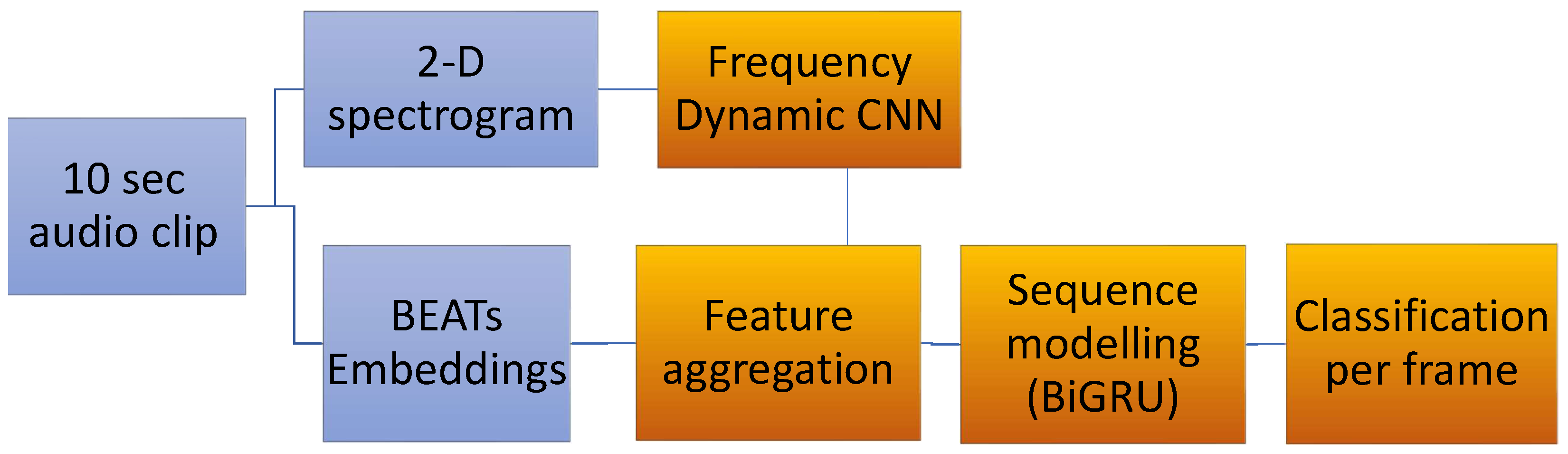
The proposed model adopts and modifies the baseline of the DCASE2023 competition by employing specific versions of the aforementioned modules. More specifically, it combines BEATs embeddings with the output of a frequency-dynamic convolution network, where an extra local attention module is added sequentially after each dynamic convolution. The combined embeddings pass through a BiGRU (bi-directional recurrent unit) unit and, finally, a classification module. The model that consists of the above modules (student) has an identical teacher model that is updated with the exponential average of the weights of students. The combination of these techniques for the SED problem is novel to the best of our knowledge and succeeds in offering a lightweight architecture with sufficient performance.

2. Dataset

This study uses the DESED dataset [5] for development, since it is provided by DCASE2023. The training data of this dataset consist of three different splits: weakly labeled training set, unlabeled in-domain training set, and synthetic strongly labeled set with strong annotations. The majority of files are 10 s clips. The weakly labeled training set (each 10 sound clip has global labels independent of the duration of the corresponding event class) contains 1578 clips (2244 class occurrences). The unlabeled in-domain training set contains 14,412 clips. Synthetic strongly labeled set (each sound event has a start and an end time in the 10 s clip) is composed of 10,000 clips, produced with the Scaper soundscape synthesis and the augmentation library. The AudioSet extra clips from the classes vacuum, blender, and cat were used in a second-stage training. These clips, together with unlabeled data, acquired strong pseudo-labels by the best first-stage trained system. The rule to include AudioSet extra clips and the strong annotations of sound events in a second-stage training was the detection of sound events by the first stage system and that the weak prediction value of the corresponding class was higher than 0.7. This resulted in the inclusion of 953 clips from the blender class, 1185 clips from the vacuum class, and 3098 clips from the cat class.

3. Methodology Overview

In this section, we present the proposed methodology of this paper, which consists of the following steps:

• Mel-spectrogram transformation;
• Data augmentation;
• Feature extraction
• Aggregation of features with embeddings;
• Sequence modeling;
• Classification per frame;
• Post-processing.

The trainable part of this system (starting from Step 3 to Step 6) is the main model, which is used as a student model in a mean teacher training scheme. An identical model, i.e., the teacher model, acquires its weights updated by the exponential moving average of student’s weights, and it is not trained directly on data. The consistency between the two models contributes to the student’s training loss. In Figure 1, the data pre-processing and the trainable part of the system, i.e., with post-processing excluded, are shown.

3.1. Mel-Spectrogram Extraction and Data Normalization

The mel-spectrogram has been used in several studies and is usually the initial feature representation in several state-of-the-art methods [7,8,9,10]. Moreover, most studies that examine domestic event detection choose the same parameters for the mel-spectrogram. In this study, the most popular parameters are adopted: number of mels: 128, FFT size: 2048, hop length: 256 samples, window length: 2048 samples, sample rate: 16,000 Hz, minimum frequency: 0 Hz, maximum frequency: 8000 Hz. This results in a mel-spectrogram with 626 time frames and 128 mel frequency bins for each 10 s clip. This resolution is considered to offer adequate detail over time and frequency and avoids an oversized input to the deep learning pipeline. Data are normalized with the min–max operation per batch. This is a common practice in domestic SED. Other batch normalization methods may affect the results, but were not tested exhaustively. In this study’s tests, min–max normalization contributed to better performance compared to mean normalization and is preferred by other studies. In addition, min–max normalization is selected to be applied over time and frequency compared to batch and frequency, since it features slightly better performance. The minimal effect of data normalization, when altering the normalization method, led to the decision to adopt min–max over time and frequency to the tests presented in this paper.

3.2. Data Augmentation

In this study, data augmentations that are applied directly to the spectrogram are used. According to [6], these techniques are easier to conceive and implement, requiring fewer computations than data augmentation techniques that are applied to the raw one-dimensional audio signal. Moreover, they are more convenient to optimize the parameters of spectrogram data augmentation techniques, and these techniques have been efficient in improving performance in sound event detection tasks [7,8,10]. The techniques that are widely adopted by efficient SED systems are specaugment, FilterAugment, mixup, time and frequency shift, and Gaussian noise addition.

Masking of time and/or frequency, in this context, refers to removing parts of the log-mel-spectrogram and leaving them empty (without any value or zero). Although the augmented instance has less information than the original clip, it assists an acoustic model in generalizing. To avoid the loss of information in the augmented spectrogram instance, FilterAugment [6] randomly weights frequency bands.

3.2.1. Data Augmentation Implementation and Application Details

FilterAugment is superior to specaugment [6], and mixup contributes to better generalization according to our tests and the state-of-the-art methods. Other augmentation techniques were not exhaustively tested, but when tested, they did not have a significant effect on results. The following data augmentations are applied to the mel-spectrogram with different combinations.

3.2.2. Mixup

Mixup combines all instances of a batch with a selected rate per batch. Commonly, half the batches are passed through mixup augmentation. If a randomly generated value between 0 and 1 surpasses the mixup ratio of 0.5, the batch passes through the mixup augmentation. The mixup operation adds the batch, multiplied by a factor c, with one random permutation of instances of its own multiplied by a factor $(1-c)$. The factor c is randomly derived from a beta distribution with parameters $\alpha =0.2$ and $\beta =0.2$. The beta distribution with such parameters has higher probabilities to produce values close to 0 or 1. This results in a small amount of mixup in most cases. This is referred to as soft mixup, while in hard mixup, the range of c is narrowed to [0.3, 0.7], resulting in a greater amount of mixup in each case.

3.2.3. FilterAugment

FilterAugment has two versions: linear and step. The main idea is that, instead of masking out a frequency band, which results in information loss, an augmented instance is created by multiplying a frequency band with a factor that either increases or decreases the corresponding spectrogram values. This is a parametric method. FilterAugment’s parameters were optimized in [6] for SED, and in this study, these values are also adopted.

3.3. Feature Extraction with Convolutional Neural Networks

In this section, the architecture of the proposed convolutional neural network will be analyzed in more detail.

3.3.1. Proposed Network Architecture for Feature Extraction

In order to extract features from interactions between frequencies and time points, a CNN with convolutional layers is common practice. Domain-specific frequency-dynamic convolution replaced the standard 2D convolution, and an extra attention module layer was placed after each convolutional layer. In

Table 1. The proposed CNN architecture “FDY-CNN-dLKA”.

Layer	Contents	Output Size
Input	-	(size: $1\times T=626\times Freq=128$)
CN	$\left[\begin{array}{c}Conv2d\left(3\right)\\ BatchNormalization\\ Activation=ContextGating\\ dLKA\\ Dropout(p=0.5)\\ AvgPool2d\end{array}\right]$	$32\times 313\times 64$
FDY1	$\left[\begin{array}{c}FDConv2d\left(3\right)\\ BatchNormalization\\ Activation=ContextGating\\ dLKA\\ Dropout(p=0.5)\\ AvgPool2d\end{array}\right]$	$64\times 156\times 32$
FDY2	$\left[\begin{array}{c}FDConv2d\left(3\right)\\ BatchNormalization\\ Activation=ContextGating\\ dLKA\\ Dropout(p=0.5)\\ AvgPool2d\end{array}\right]$	$128\times 156\times 16$
FDY3	$\left[\begin{array}{c}FDConv2d\left(3\right)\\ BatchNormalization\\ Activation=ContextGating\\ dLKA\\ Dropout(p=0.5)\\ AvgPool2d\end{array}\right]$	$256\times 156\times 8$
FDY4	$\left[\begin{array}{c}FDConv2d\left(3\right)\\ BatchNormalization\\ Activation=ContextGating\\ dLKA\\ Dropout(p=0.5)\\ AvgPool2d\end{array}\right]$	$256\times 156\times 4$
FDY5	$\left[\begin{array}{c}FDConv2d\left(3\right)\\ BatchNormalization\\ Activation=ContextGating\\ dLKA\\ Dropout(p=0.5)\\ AvgPool2d\end{array}\right]$	$256\times 156\times 2$
FDY6	$\left[\begin{array}{c}FDConv2d\left(3\right)\\ BatchNormalization\\ Activation=ContextGating\\ dLKA\\ Dropout(p=0.5)\\ AvgPool2d\end{array}\right]$	$256\times 156\times 1$

, the proposed frequency-dynamic CNN-downsized large-kernel attention (FDY-CNN-dLKA) is presented. In addition, the proposed task-specific modules FDY and dLKA are explained.

3.3.2. Frequency-Dynamic Convolution

There are several hyperparameters of the frequency-dynamic convolution network that can be fine-tuned [7]. In this study, we use the optimal hyperparameters proposed in [7] without modification, since they were optimized for SED. In addition, an improvement in the FDY-CNN network was proposed by [8], and this implementation was also tested in experiments in this study. The implementation of the developed FDY-CNN is the following. The FDY-CNN is a CNN, where some or all of its convolutional layers are frequency-dynamic convolutional (FDC) layers. An FDC performs convolution with frequency-adaptive attention weights, which occur by the processes described in

Table 2. Extraction of the attention weights. $C_{in}$ is the number of input channels for each dynamic convolution, $Freq$ is the number of frequency bins, $h_c$ is the number of intermediate hidden channels, K is the number of basis kernels, and ${\pi }_i\left(f\right)$ is the weights to extract.

Layer	Contents	Output Size
Input Features		$C_{in}\times T\times Freq$
Average Pool time	AveragePooling	$C_{in}\times 1\times Freq$
Conv1d1	conv1d(3)	$Hidchan\times Freq$
${\pi }_i\left(f\right)$ Calculation	$\begin{array}{c}BatchNormalization\\ Activation=ReLU\\ conv1d\left(3\right)\\ softmax(x/temperature,1)\end{array}$	$K\times Freq$

. The outcome of these processes is the frequency-adaptive attention weights, denoted as ${\pi }_i$, where i is the corresponding basis kernel. Then, convolutions are performed according to the following equations:

$$y_i(t,f)=W_i\ast x(t,f)+b_i$$

(1)

$$\mathcal{Y}(t,f,x)=\sum _{i=1}^K{\pi }_i(f,x)y_i(t,f)$$

(2)

where $W_i$ is the weights for the corresponding basis kernel i, $b_i$ is the bias, $x(f,t)$ is the layer input, $\mathcal{Y}$($t,f,x$) is the final output of the FDC layer, and K is the number of basis kernels.

3.3.3. Downsized Large-Kernel Attention

Frequency-dynamic convolution (FDC) and multidimensional frequency-dynamic convolution (MFDC) are modules that apply attention to the kernel level. Due to the limited amount of data and the short duration of certain sound events, local-level attention has been shown to be more effective than global attention, which is applied to the spectrogram of the 10 s clip. Although FDC and MFDC are specialized to extract spectrogram features, other attention modules can be as effective. Large-kernel attention (LKA) is an attention module that is effective in computer vision [23]. Experiments were conducted, testing the following combinations: FDC-LKA and MFDC-LKA. The development set results show that FDC-LKA can generalize better and thus perform better. Although large-kernel attention has a submodule of dilated convolution to effectively expand the kernel size, in the application of the CNN for feature extraction, each frequency-dynamic convolution has a $3\times 3$ kernel. Therefore, the proposed LKA module is downsized to capture the same kernel size. This results eventually in a small kernel attention, and it is referred to as dLKA in Table 1.

In Figure 2, dKLA is presented. On the left, the flowchart is shown. In the middle, the components of attention and FFN are presented. On the right, the module that is referred to as LKA in [23] is presented in detail. The whole module uses attention and a feedforward component. Convolutions are decomposed to reduce the computations. The key part of the attention module “dLKA” (on the right of Figure 2) is that it uses a depth-wise convolution to capture spatial local information, a depth-wise and dilated convolution to extend the kernel range and 1 × 1 point-wise convolution on the channel dimension to offer channel-adaptability.

3.4. BEATs Embeddings

The bi-directional encoder representation from audio transformers (BEATs) embeddings revolutionized general (non-speech and non-music) audio self-supervised learning by introducing representations that are learned for discrete-level prediction, instead of relying solely on reconstruction loss. This allows for high-level feature extraction that contains richer semantic information. At the inference level, only the transformer encoder of the whole BEATs self-supervised learning model can be used. With the addition of a classifier, it can predict patch-based discrete labels. This encoder is a ViT transformer [24] with 12 encoder layers, 8 attention heads, and 768-dimensional hidden states (model size: 90 M parameters).

The network receives as input acoustic spectrogram features, which occur as proposed by Gong et al. [25]. Specifically, the raw waveform is resampled to 16.000 Hz, and 128-dimensional mel-filter bank features are extracted with a 25 ms Povey window that hops every 10 ms. The features are normalized to the mean value of 0 and the standard deviation of 0.5. Finally, acoustic features for each clip are split into the $16\times 16$ patches.

The BEATs embeddings are extracted from the BEATs transformer, which is trained in a self-supervised manner, described in [16], on AudioSet and has an output size of $496\times 768$ size per 10 s clip. In order to leverage the representation capability of BEATs embeddings, in this study, they are combined with other learnable representations (outcome of FDY-CNN-LKA), while the BEATs transformer is kept frozen and extracts only the initial embeddings of the DESED dataset.

3.5. Combining Embeddings

BEATs embeddings have a size of $496\times 768$ per audio clip, while the outcome of FDY-NN is $256\times 156$. It has been proven that it is effective to concatenate these representations before passing them through a sequence modeling module [9,26], which is a bi-directional GRU in most cases. Two methods are commonly used to merge the two representations into one. These are described as follows:

• Adaptive average pooling of one dimension of BEATs and dense reduction: After 1-D adaptive average pooling, the shape of the embedding becomes $768\times 156$. After transposition (156,768), the embedding is concatenated with FDY-CNN features along the frame axis, and the outcome has shape $156\times (768+256)$. Then, it passes through a dense layer to be reduced to the FDY-CNN features shape $256\times 156$.
• Interpolate the BEATs embedding as an image with mode “nearest-exact”: In this case, the embedding also becomes $768\times 156$ because this is the target shape of interpolation. Afterwards, the process is the same as for adaptive average pooling, and the result is a $256\times 156$ feature shape

3.6. Bigru and Classification Layer

After the concatenation of CNN features and embeddings, the outcome passes through a bi-directional gated recurrent unit with cell size of 256, a dropout, and the final classification layer. As shown in Figure 3, an attention module is applied to produce the weak clip-level predictions, which take into account the strong frame-wise predictions.

3.7. Mean Teacher–Student Model

Various methods have been proposed to leverage the unlabeled data. One very common and efficient method is the mean average teacher–student model [19]. In this scheme, the student model’s weights are updated according to calculated losses in each training iteration, while the teachers’ weights are updated by the weighted average of the student’s model weights. The student model has to be consistent with the predictions of the teacher on the unlabeled data. A consistency loss between the student’s and teacher’s predictions is calculated in each iteration and is aggregated in supervised loss to update the student’s weights only. Consistency loss gets a global weight that is increased in each iteration, as the predictions of students and teachers should be more meaningful when the models have been trained enough in a supervised manner. The choices for consistency loss that were tested in this study were the mean squared error loss, the binary cross-entropy loss, and the weighted binary cross-entropy loss (implementation of confident mean teacher [8]). The mean teacher scheme results in a teacher model more capable of generalizing. Results refer to the outcome of the teacher model, which was superior to the student’s in every conducted experiment. Strong predictions for each clip are a matrix with dimensions $batc{h}_{s}ize\times classes\times tim{e}_{f}rames$. For each element of strong predictions of teacher y and student model $x,$ the binary cross-entropy (BCE) loss is calculated as follows:

$$l_n=y_n\ast log{x}_n+(1-y_n)\ast log(1-x_n)$$

(3)

Then, the strong self-supervised or strong consistency loss is the average of the losses for all elements of the strong predictions matrix. Weak predictions for each clip are a matrix with dimensions $batc{h}_{s}ize\times classes$. The weak self-supervised or weak consistency loss is calculated in an analogous way to the strong consistency loss. Finally, the consistency losses are aggregated to the supervised loss.

3.8. Post-Processing

Post-processing smooths the development test dataset outcome after the model training. Only in the case of the CMT experiment, post-processing (same as in testing) is used to the teacher model’s outcome per iteration in order to train the student to more confident predictions. Median filtering along the time axis is a common practice to take into account the continuous nature of sound events. Due to the differences in duration of sound events, e.g., a dog barking can be an instantaneous event, while running water usually has a long duration, a specific length of median filtering is used for each category. Recently, Ebbers et al. [27] published an article examining the effect of post-processing in domestic SED and applying a post-processing independent metric for the outcome. It was shown that there may be a trade-off between PSDS1 and PSDS2 scores, and post-processing may enhance PSDS2 but deteriorate PSDS1. However, in this study, results are presented with the aforementioned post-processing.

3.9. Model Training

The batch size contained 24 weak-labeled, 24 strong-labeled, and 48 unlabeled clips. All experiments that are presented were conducted using binary cross-entropy (BCE) as supervised loss. The supervised loss is the sum of the supervised loss for strong frame-wise predictions and the supervised loss for weak clip-wise predictions. For consistency loss, i.e., the loss between students’ and teachers’ predictions, BCE was also used in every experiment except for one where weighted BCE was also tested [8] to compare its performance. The optimizer that was used for training was AdamW [28]. The proposed model was retrained using additional AudioSet clips and unlabeled DESED data with strong pseudolabels.

4. Results

4.1. Implementation

The proposed method was implemented in Python v3.8.10 using the scikit-learn package. The deep learning architectures were developed in Python v3.8.10 and PyTorch and PyTorch Lightning. For the experiments, we used an Ubuntu 22.04 PC with 64GB RAM, an Intel i9-11900KF 3.5 GHz CPU, and an NVIDIA RTX A6000 GPU with 48 GB of RAM.

4.2. Metrics

The polyphonic sound event detection (PSDS) score has been used since its introduction in 2019 [29] in this specific task, along with the F1-macro, F1-micro, segment-based scores, event-based scores, and/or intersection-based score. The PSDS score is an extension to event-based and intersection-based scores and is currently the most widely used metric in domestic sound event detection. In short, its advantages are robustness against labeling subjectivity, better insight into the model performance (by using receiver operating characteristic (ROC) curves), and classification stability across classes. One of the main attributes of PSDS is that it is threshold-independent. Bilen et al. [29] used arbitrary thresholds to approximate it. Due to the large number of possible thresholds, Ebbers et al. [30] proposed a method to approximate continuous PSDS-ROC curves (as if all possible thresholds are used).

4.3. Comparison with Other Methods

In

Table 3. A comparison between the proposed method (in bold) and recent efficient methods. The results refer to development test set.

Model	PSDS1	PSDS2	Event F1-Macro	No. Parameters	No. Models
FDYCRNNdLKA	0.515	0.798	0.613	5M	1
FDYCRNNdLKA (Second-stage training)	0.53	0.8	0.613	5M	1
FDY-CRNN	0.452	0.672	0.54	3M	1
MFD -CMT	0.470	0.692	0.548	3.5M	1
Kim et al. [9]	0.527	0.782	0.633	9M	1
Kim et al. (Second-stage training) [9]	0.546	0.808	0.638	9M	1
Kim et al. (ensemble) [9]	0.567	0.815	0.656	9×46M	46
Zhang et al. [26]	0.562	0.830	-	240M	25

, the proposed method with the acronym FDYCRNNdLKA is compared with other recent efficient methods, including the best and second-best submission in the DCASE 2023 challenge. It is obvious that the winning submissions and the proposed method are boosted by the inclusion of BEATs embeddings. FDY-CRNN and MFD-CMT are the bases for other methods but do not use BEATs embeddings. Winning submissions included the ensemble of many models and had superior performance to the proposed, which is a single model. However, Kim et al. [9] report development test set results on a single model. Its best single model has a larger PSDS1 score of 0.527 than 0.515, i.e., the PSDS1 score of the proposed model, while the proposed model performs better with a PSDS2 score of 0.798 compared to 0.782. In the second stage, training Kim et al. [9] method is more enhanced and performs better in each metric. This is due to more confident predictions on unlabeled data, which are produced by an ensemble of six models, as reported in [9] and are used in the second stage of training. The proposed model has a better performance for a single model in PSDS2 score and has nearly half the parameters (5M) of the parameters used in the single model of Kim et al. [9].

In

Table 4. A comparison of complexities of recent efficient methods.

Model	Energy Consumption kWH	MACS	No of Trainable Parameters	Training Time	GPU
FDYCRNNdLKA	3.18	1.851B	5M	9 h 42 m	1 RTX A6000
FDYCRNNdLKA (2nd stage training)	2.24	1.851B	5M	7 h	1 RTX A6000
Kim et al. [9]	3.91	7B	9M	14 h 36 m	4 RTX A6000
Kim et al. (2nd stage training) [9]	2.78	7B	9M	15 h 31 m	4 RTX A6000
Zhang et al. (single model) [26]	20.48	368B	9M	6 h	1 Tesla A100

, metrics for the energy consumption and complexity are presented for the proposed method and state-of-the-art single models from Table 3. The proposed method requires less multiply-accumulate operations (MACS) and less energy consumption for training, according to the reported measurements from codeCarbon for the DCASE2023. However, the use of one GPU instead of four GPUs for less time indicates that the energy consumption could be significantly less than the other state-of-art methods. Table 4 shows that the proposed method is lighter and less energy-consuming, but there is room for augmenting the capacity of the model without increasing the complexity too much.

4.4. Ablation Study

An ablation study was conducted to examine the effect of data augmentation, feature extraction components, and parameters concerning self-supervised learning and training, e.g., the choice of consistency loss and the choice of optimizer.

4.4.1. Data Augmentation Techniques

In

Table 5. A performance overview of the data augmentation techniques used (best value in bold).

Model	PSDS1	PSDS2	Event F1-Macro	Intersection F1-Macro
No augmentation	0.492	0.784	0.576	0.795
Soft mixup (rate 50 %)/embeddings augmented	0.499	0.772	0.577	0.802
Soft mixup (rate 50 %)	0.511	0.776	0.584	0.804
Soft mixup (rate100 %)	0.507	0.77	0.58	0.798
Hard mixup (rate 50 %)	0.503	0.79	0.598	0.81
Hard mixup (rate 50 %) + FiltAugment	0.508	0.787	0.587	0.807

, results for different data augmentation setups are shown. Applying soft mixup to embeddings did not alter the results significantly, while soft mixup to half of the batch clips improved the PSDS1 score from 0.492 to 0.511. Therefore, the rest of the experiments were conducted with no mixup to the embeddings. Soft mixup to all of the samples was not as efficient as the softmax to half the batch’s clips. Hard mixup improved the PSDS2 score and the event-based and intersection-based F1-score, but was not as efficient as soft mixup in enhancing the PSDS1 score. However, it was considered more balanced in enhancing the results and in combination with filtAugment was chosen as the data augmentation for the proposed method and for the following. It can be inferred from this table that there is a trade-off between PSDS1 and PSDS2, and a data augmentation may enhance the one and deteriorate the other.

4.4.2. Feature Extraction

In

Table 6. A performance overview of the tested models (best values on bold).

Model	PSDS1	PSDS2	Event F1-Macro	Intersection F1-Macro	No. Parameters
CNNFDY	0.513	0.795	0.613	0.823	3M
CNNFDY-LKA	0.504	0.79	0.6	0.824	5M
CNNFDY-LKA-original-(dropout 0.5 after LKA module/large)	0.506	0.792	0.594	0.827	9M
CNNMFDY-LKA	0.505	0.797	0.607	0.829	9M
FDYCRNNdLKA (dropout 0.5 after LKA module)	0.515	0.798	0.613	0.831	5M

, experimental results for different model architectures are shown. The first model CNNFDY is the model as presented in [7] without the LKA module. The second model CNNFDY-LKA has the LKA module placed after the activation and in between Dropout and AvgPool2d, (see Table 1). The model CNNFDY-LKA-original has the LKA module in between Activation and Dropout and has the double features maps of all other models. The model CNNNFDY-LKA-downsized has a downsized LKA module in between Activation and Dropout. It can be observed that only in CNNFDY-LKA-downsized, the LKA module improves the PSDS2 score compared to CNNFDY, while the PSDS1 score has minimal differences between the two models for feature extraction. Although the improvement is small, the LKA module does not add too many parameters, and CNNFDY-LKA-downsized is the proposed submodel for feature extraction. The last model of Table 6 is the proposed model that is referred to in Table 3 as FDYCRNNdLKA (first-stage training).

4.4.3. Self-Supervised Learning

Concerning self-supervised learning, the consistency loss between student’s and teacher’s predictions was calculated in two different ways. In

Table 7. Different consistency loss between student’s and teacher’s predictions (best values in bold).

Model	PSDS1	PSDS2	Event F1-Macro	Intersection F1-Macro
BCE	0.513	0.795	0.613	0.823
weighted BCE	0.504	0.79	0.6	0.824

, a confident mean teacher with weighted binary cross-entropy method is compared with a simple binary cross-entropy implementation. PSDS scores were higher for BCE, and it was the design choice for the proposed model.

5. Discussion

A lightweight and efficient for domestic sound event detection is presented in this work. Various data augmentation techniques, feature extraction models, and self-supervised techniques were tested to optimize the outcome.

Concerning data augmentation, soft mixup, hard mixup, and filtAugment, which were tested in this study, were already proposed, and they are optimized for SED as independent units. Moreover, Gong et al. [25] proposed model-agnostic data manipulation for SED, which included data augmentation. However, filtAugment is a new technique and evolved with a second edition, and different combinations of these data augmentation techniques with the proposed model, had to be tested to adopt the most efficient augmentation. In addition, in the presented experiments, it can be observed that while soft mixup enhances PSDS1 and hard mixup enhances PSDS2, there are other combinations that can be more efficient.

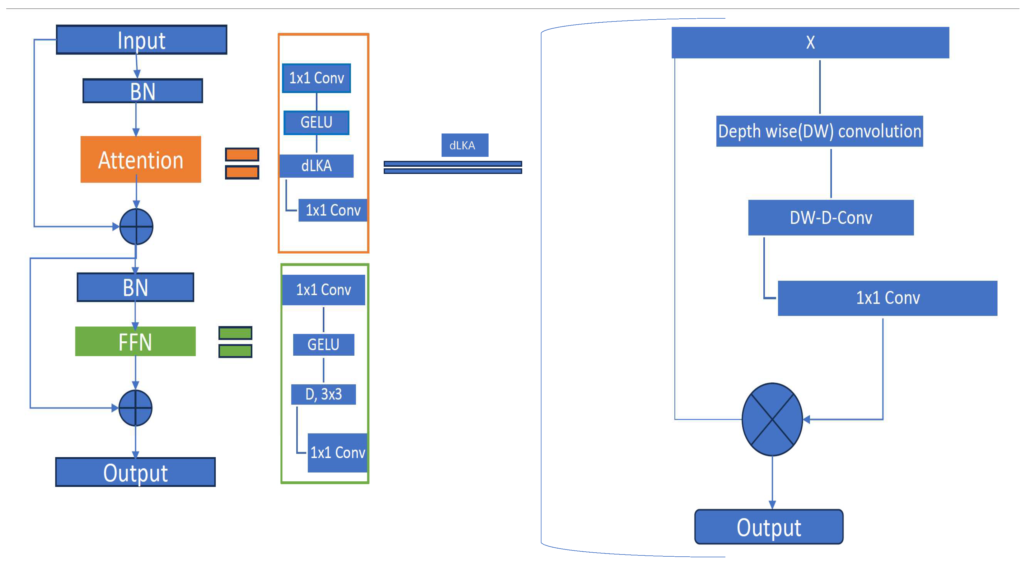
Feature extraction is the core of this method, and it was the main subject of research in domestic SED. Recent methods of frequency-dynamic convolution and multi-dimensional frequency-dynamic convolution achieved the main enhancement in results, while the rest of the SED systems had little modifications. Frequency-dynamic convolution cancels the shift-invariant nature of the convolution, while it can be considered an attention module. Attention is a hot concept in deep learning and a desired aspect of detection systems. Due to the short duration of sound events and the relatively small dataset, a global application of attention, such as the one provided by transformers, does not seem to be as efficient as local attention. In this rationale, the LKA module can be considered as a local attention module, especially when downsized to small kernel sizes. However, the enhancement in results is not so impressive, when adding LKA to frequency-dynamic convolution. Although two local attention modules in sequence may seem to have enough capacity to capture local interactions, more research can be conducted in local attention modules to be added to the effective spectrogram-specific frequency-dynamic convolution.

Another field of significant interest in domestic SED is the use of pre-trained embeddings due to the great number of AudioSet sound clips and the relatively small DESED dataset. Embeddings up to lately have relied on reconstruction loss and not discrete-level predictions. Discrete-level prediction self-supervised learning was easier to implement in music and in speech, but not in the sound events of very varying duration and frequency characteristics. BEATs embeddings achieved self-supervised with discrete-level prediction by starting the training with random discrete labels and iteratively adapting them to the encoding system, which was a transformer. The pre-trained BEATs embeddings significantly boosted the performance of various domestic SED systems when aggregated to the features extracted by CNNs and are adopted in this study. The key idea of self-supervised learning is training on discrete labels in the iterative scheme, proposed in [16] and thus extracting higher-level features semantically richer. It is probable that research in altering the ViT transformer with another encoder in BEATs training scheme may produce embeddings with more capacity for a specific task like domestic SED.

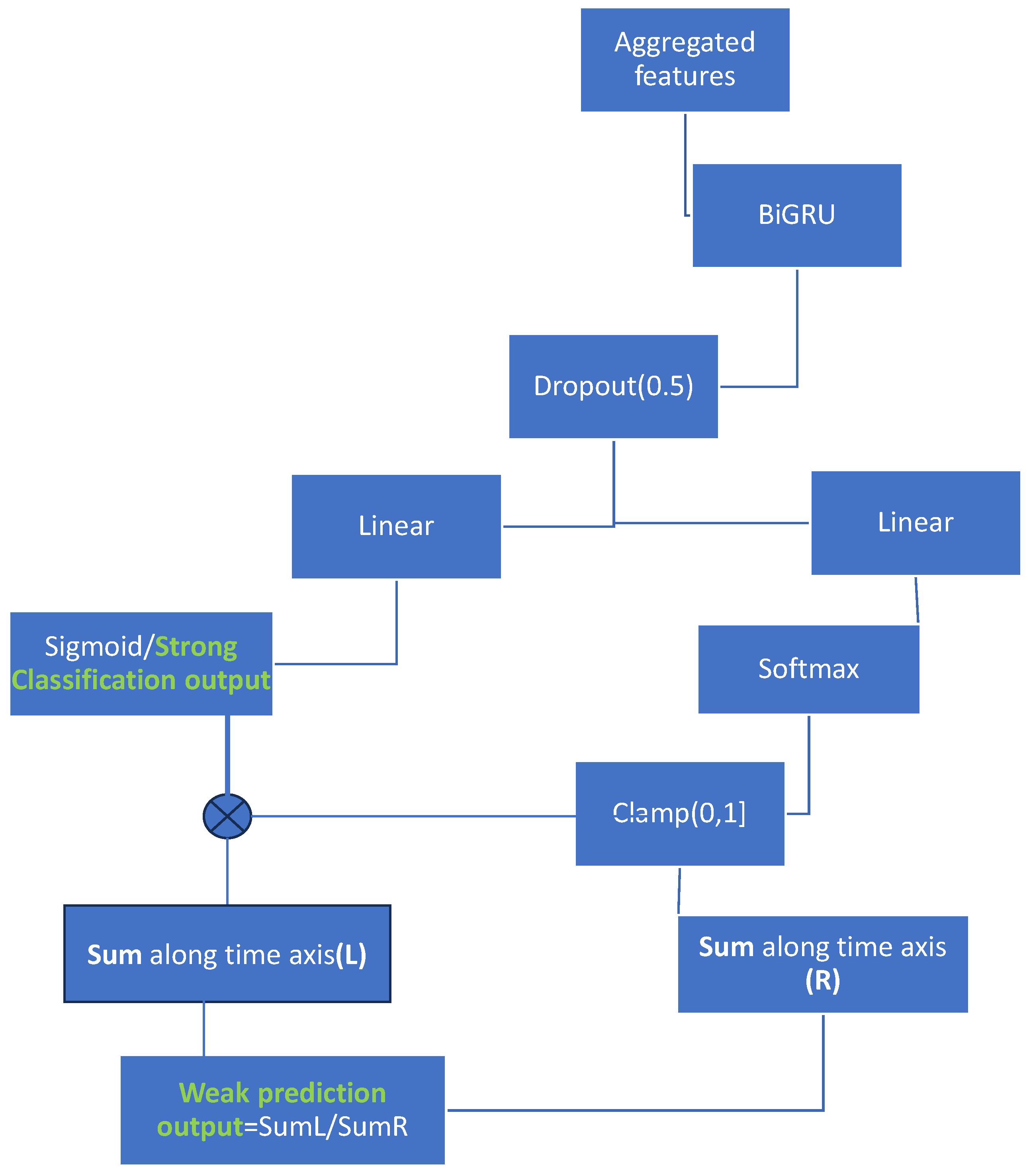
As stated before, global attention did not improve results in domestic SED. Specifically, several research efforts have proposed various transformers in place of BiGRU or other RCNN. However, BiGRU, which demands fewer computations and memory, is to the best of our knowledge, more efficient to this date. Recently, a technique called glance-and-focus [31] was published, which also uses the attention and transformer architectures. The aim is to locate an anomaly event in a long video sequence. In this approach, global attention is applied first and then local attention. This sequentially applied attention could also be applied in DESED. However, in DESED, there are 10 classes that may have any duration, and there is no notion of normality. The classification layer in the proposed method of this paper uses global attention to extract weak labels (Figure 3). In a sense, the proposed method first uses local attention with dLKA and then global attention in a reverse manner to [31].

Ensemble models have also proved efficient in various works. However, they demand many computational resources and many hours or days of training. This study focuses on finding an efficient single model, and this could be the basis of ensemble models that can be less than 50 models, as it is common in the winning systems of DCASE. Moreover, there is also concern about the environmental consequences of training large and complex systems.

The novelty of this method is the combination of state-of-the-art modules, which are adapted in a suitable way to perform the SED task. This combination is not encountered in the literature to the best of our knowledge. Several ablation tests were presented in the text that demonstrate that the proposed combination yields optimal performance.

6. Conclusions

A lightweight single-model method, which achieves better performance in the PSDS2 score and comparable performance in the PSDS2 score with state-of-the-art single models while using a significantly smaller number of parameters was presented. PSDS2 score performance is important for monitoring of domestic activities of the elderly because its goal is the detection/classification of long-lasting sound events with accurate predictions and avoidance of misclassifications. Performance in the PSDS1 score is comparable to state-of-the-art single models and also indicates the potential of the system to be used as an alarm.

References

1. Debes, C.; Merentitis, A.; Sukhanov, S.; Niessen, M.; Frangiadakis, N.S.; Bauer, A. Monitoring activities of daily living in smart homes: Understanding human behavior. IEEE Signal Process. Mag. 2016, 33, 81–94. [Google Scholar] [CrossRef]
2. Fleury, A.; Vacher, M.; Noury, N. SVM-based multimodal classification of activities of daily living in health smart homes: Sensors, algorithms, and first experimental results. IEEE Trans. Inform. Technol. Biomed. 2010, 14, 274–283. [Google Scholar] [CrossRef] [PubMed]
3. Popescu, M.; Li, Y.; Skubic, M.; Rantz, M. An acoustic fall detector system that uses sound height information to reduce the false alarm rate. In Proceedings of the 30th Annual International Conference of the IEEE Engineering in Medicine and Biology Society, Vancouver, BC, Canada, 20–25 August 2008; pp. 4628–4631. [Google Scholar]
4. Gemmeke, J.F.; Ellis, D.P.W.; Freedman, D.; Jansen, A.; Lawrence, W.; Moore, R.C.; Plakal, M.; Ritter, M. Audio Set: An ontology and human-labeled dataset for audio events. In Proceedings of the 2017 IEEE International Conference on Acoustics, Speech and Signal Processing (ICASSP), New Orleans, LA, USA, 5–9 March 2017; pp. 776–780. [Google Scholar] [CrossRef]
5. Serizel, R.; Turpault, N.; Shah, A.; Salamon, J. Sound event detection in synthetic domestic environments. In Proceedings of the ICASSP 2020–2020 IEEE International Conference on Acoustics, Speech and Signal Processing (ICASSP), Barcelona, Spain, 4–8 May 2020; pp. 86–90. [Google Scholar]
6. Nam, H.; Kim, S.H.; Park, Y.H. Filteraugment: An acoustic environmental data augmentation method. In Proceedings of the ICASSP 2022–2022 IEEE International Conference on Acoustics, Speech and Signal Processing (ICASSP), Singapore, 22–27 May 2022; pp. 4308–4312. [Google Scholar]
7. Nam, H.; Kim, S.H.; Ko, B.Y.; Park, Y.H. Frequency Dynamic Convolution: Frequency-Adaptive Pattern Recognition for Sound Event Detection. In Proceedings of the Interspeech 2022, Incheon, Republic of Korea, 18–22 September 2022; pp. 2763–2767. [Google Scholar]
8. Xiao, S.; Zhang, X.; Zhang, P. Multi-Dimensional Frequency Dynamic Convolution with Confident Mean Teacher for Sound Event Detection. In Proceedings of the ICASSP IEEE International Conference on Acoustics, Speech and Signal Processing (ICASSP), Rhodes Island, Greece, 4–10 June 2023; pp. 1–5. [Google Scholar]
9. Kim, J.W.; Son, S.W.; Song, Y.; Kim; Kook, H.; Song, I.H.; Lim, J.E. Semi-supervised learning-based sound event detection using frequency dynamic convolution with large kernel attention for DCASE challenge 2023 task 4. arXiv 2023, arXiv:2306.06461. [Google Scholar]
10. Shao, N.; Loweimi, E.; Li, X. RCT: Random Consistency Training for Semi-supervised Sound Event Detection. arXiv 2021, arXiv:2110.11144. [Google Scholar]
11. Koh, C.-Y.; Chen, Y.-S.; Liu, Y.-W.; Bai, M.R. Sound Event Detection by Consistency Training and Pseudo-Labeling with Feature-Pyramid Convolutional Recurrent Neural Networks. In Proceedings of the ICASSP 2021—2021 IEEE International Conference on Acoustics, Speech and Signal Processing (ICASSP), Toronto, ON, Canada, 6–11 June 2021; pp. 376–380. [Google Scholar] [CrossRef]
12. Kim, S.J.; Chung, Y.J. Multi-Scale Features for Transformer Model to Improve the Performance of Sound Event Detection. Appl. Sci. 2022, 12, 2626. [Google Scholar] [CrossRef]
13. Miyazaki, K.; Komatsu, T.; Hayashi, T.; Watanabe, S.; Toda, T.; Takeda, K. Conformer-based Sound event detection with semi-supervised learning and data augmentation. In Proceedings of the Detection and Classification of Acoustic Scenes and Events 2020, Tokyo, Japan, 2–3 November 2020. [Google Scholar]
14. Du, Q.; Luo, Y. You Only Look & Listen Once: Towards Fast and Accurate Visual Grounding. In Proceedings of the 2022 IEEE 42nd International Conference on Distributed Computing Systems Workshops (ICDCSW), Bologna, Italy, 10–13 July 2022; pp. 139–144. [Google Scholar]
15. Niizumi, D.; Takeuchi, D.; Ohishi, Y.; Harada, N.; Kashino, K. Byol for audio: Self-supervised learning for general-purpose audio representation. In Proceedings of the 2021 International Joint Conference on Neural Networks (IJCNN), Shenzhen, China, 18–22 July 2021; pp. 1–8. [Google Scholar]
16. Chen, S.; Wu, Y.; Wang, C.; Liu, S.; Tompkins, D.; Chen, Z.; Wei, F. BEATs: Audio Pre-Training with Acoustic Tokenizers. arXiv 2022, arXiv:2212.09058. [Google Scholar]
17. Cho, Κ.; Merriënboer, B.V.; Gulcehre, C.; Bahdanau, D.; Bougares, F.; Schwenk, H.; Bengio, Y. Learning phrase representations using RNN encoder-decoder for statistical machine translation. arXiv 2014, arXiv:1406.1078. [Google Scholar]
18. Ashish, V.; Shazeer, N.M.; Parmar, N.; Uszkoreit, J.; Jones, L.; Gomez, A.N.; Kaiser, L.; Polosukhin, I. Attention is All you Need. In Proceedings of the Conference on Neural Information Processing Systems (NeurIPS), Long Beach, CA, USA, 4–9 December 2017. [Google Scholar]
19. Tarvainen, A.; Valpola, H. Mean teachers are better role models: Weight-averaged consistency targets improve semi-supervised deep learning results. Adv. Neural Inf. Process. Syst. 2017, 2017, 1196–1205. [Google Scholar]
20. Duo, X.; Fang, W.; Li, J. Semi-Supervised Sound Event Detection System for DCASE 2023 Task4a. DCASE2023 Challenge. Technical Report June 2023. Available online: https://dcase.community/documents/challenge2023/technical_reports/DCASE2023_Wenxin_97_t4a.pdf (accessed on 28 September 2023).
21. Chen, K.; Du, X.; Zhu, B.; Ma, Z.; Berg-Kirkpatrick, T.; Dubnov, S. HTS-AT: A Hierarchical Token-Semantic Audio Transformer for Sound Classification and Detection. In Proceedings of the ICASSP 2022—2022 IEEE International Conference on Acoustics, Speech and Signal Processing (ICASSP), Singapore, 23–27 May 2022; pp. 646–650. [Google Scholar] [CrossRef]
22. Gulati, A.; Qin, J.; Chiu, C.-C.; Parmar, N.; Zhang, Y.; Yu, J.; Han, W.; Wang, S.; Zhang, Z.; Wu, Y.; et al. Conformer: Convolution-augmented transformer for speech recognition. arXiv 2020, arXiv:2005.08100. [Google Scholar]
23. Guo, M.H.; Lu, C.; Liu, Z.N.; Cheng, M.M.; Hu, S. Visual attention network. Comp. Visual Media 2023, 9, 733–752. [Google Scholar] [CrossRef]
24. Arnab, A.; Dehghani, M.; Heigold, G.; Sun, C.; Lucic, M.; Schmid, C. Vivit: A Video Vision Transformer. In Proceedings of the IEEE/CVF International Conference on Computer Vision (ICCV), Online, 11–17 October 2021. [Google Scholar]
25. Gong, Y.; Chung, Y.-A.; Glass, J. Psla: Improving audio tagging with pretraining, sampling, labeling, and aggregation. IEEE/ACM Trans. Audio Speech Lang. Process. 2021, 29, 3292–3306. [Google Scholar] [CrossRef]
26. Xiao, S.; Shen, J.; Hu, A.; Zhang, X.; Zhang, P.; Yan, P.Y. Sound Event Detection with Weak Prediction for DCASE 2023 Challenge Task4A, DCASE2023 Challenge. Technical Report, June 2023. Available online: https://dcase.community/documents/challenge2023/technical_reports/DCASE2023_Zhang_63_t4a.pdf (accessed on 28 September 2023).
27. Ebbers, J.; Haeb-Umbach, R.; Serizel, R. Post-Processing Independent Evaluation of Sound Event Detection Systems. arXiv 2023, arXiv:2306.15440. [Google Scholar]
28. Loshchilov, I.; Hutter, F. Decoupled Weight Decay Regularization. In Proceedings of the International Conference on Learning Representations, Toulon, France, 24–26 April 2017. [Google Scholar]
29. Bilen, C.; Ferroni, G.; Tuveri, F.; Azcarreta, J.; Krstulović, S. A Framework for the Robust Evaluation of Sound Event Detection. In Proceedings of the ICASSP 2020—2020 IEEE International Conference on Acoustics, Speech and Signal Processing (ICASSP), Barcelona, Spain, 4–8 May 2020; pp. 61–65. [Google Scholar]
30. Ebbers, J.; Serizel, R.; Haeb-Umbach, R. Threshold independent evaluation of sound event detection scores. In Proceedings of the ICASSP 2022—2022 IEEE International Conference on Acoustics, Speech and Signal Processing (ICASSP), Singapore, 23–27 May 2022; pp. 1021–1025. [Google Scholar]
31. Chen, Y.; Liu, Z.; Zhang, B.; Fok, W.; Qi, X.; Wu, Y.-C. MGFN: Magnitude-Contrastive Glance-and-Focus Network for Weakly-Supervised Video Anomaly Detection. Proc. AAAI Conf. Artif. Intell. 2023, 37, 387–395. [Google Scholar] [CrossRef]
Figure 1. A flowchart of the proposed model (including feature extraction). The blocks with trainable parameters are depicted in orange color. Two such models are used (student and teacher). The two models are identical. Only the student model is trained on data. The teacher model acquires its weights from a moving average of the student’s weights.
Information 14 00534 g001
Figure 2. The dLKA module that is used (its flowchart is on the left) takes its name from the submodule on the right. In the orange and the green boxes, the submodules attention and FFN are presented in detail. The submodule dLKA is actually the main part of the attention module (orange box).
Information 14 00534 g002
Figure 3. A flowchart of the sequence modeling of aggregated features (CNN features and BEATs embeddings) and classification layer for strong and weak predictions.
Information 14 00534 g003