Abstract
Despite the efforts of the World Health Organization, blood transfusions and delivery are still the crucial challenges in blood supply chain management, especially when there is a high demand and not enough blood inventory. Consequently, reducing uncertainty in blood demand, waste, and shortages has become a primary goal. In this paper, we propose a smart platform-oriented approach that will create a robust blood demand and supply chain able to achieve the goals of reducing uncertainty in blood demand by forecasting blood collection/demand, and reducing blood wastage and shortage by balancing blood collection and distribution based on an effective blood inventory management. We use machine learning and time series forecasting models to develop an AI/ML decision support system. It is an effective tool with three main modules that directly and indirectly impact all phases of the blood supply chain: (i) the blood demand forecasting module is designed to forecast blood demand; (ii) blood donor classification helps predict daily unbooked donors thereby enhancing the ability to control the volume of blood collected based on the results of blood demand forecasting; and (iii) scheduling blood donation appointments according to the expected number and type of blood donations, thus improving the quantity of blood by reducing the number of canceled appointments, and indirectly improving the quality and quantity of blood supply by decreasing the number of unqualified donors, thereby reducing the amount of invalid blood after and before preparation. As a result of the system’s improvements, blood shortages and waste can be reduced. The proposed solution provides robust and accurate predictions and identifies important clinical predictors for blood demand forecasting. Compared with the past year’s historical data, our integrated proposed system increased collected blood volume by 11%, decreased inventory wastage by 20%, and had a low incidence of shortages.
1. Introduction
Improving supply chain performance is a critical challenge for global healthcare systems. Because it is closely related to human health, compared to other industries, the health sector has the most complex supply chains. However, in recent years, the emphasis in the health care community has been on strengthening supply networks [1,2]. One of the main reasons for this attention is to cut healthcare spending and waste, while preserving standards of customer service, reducing risks [1]. According to Privett and Gonsalvez [2], the key challenges in the health supply chain include demand uncertainty, inventory management, expiration, and a shortage of resources. Furthermore, because significant amounts of blood are wasted, it is very difficult to manage the supply chain of sensitive blood products, such as platelets, in the best way [3]. This is particularly necessary if the product has a short shelf life. Furthermore, health workers who estimate demand and make ordering estimations are usually inexperienced in complex statistical analysis and economic approaches, but rather are medical staff or have a tremendous workload in the case of trained personnel and lack of time to adopt new methodologies or put the new techniques into practice, as well as time-consuming analytics [2]. This indicates that the statistical methods used for prediction and scheduling should be straightforward to understand and implement for the typical practitioner, requiring more investment in the new advanced tools.
Addis et al. [4] emphasize the need to consider a solution’s resilience, efficacy, cost, and simplicity of application before implementing a technique that involves a specialist’s expertise. Effective forecasts of blood demand are one of the most critical inputs for making effective decisions related to the facilitation and control of blood stocks. It is also important to collect data over several years to estimate future daily and monthly seasonal demand and discover accurate information about the characteristics and types of demand [5,6,7].
The main focus of this work’s proposed solution was on the analysis and optimization of the collection stage of the blood supply chain literature review studies [8,9,10,11]. Baş Güre et al. [8] provides the most specific taxonomy, discusses current literature on the collection process, and identifies research gaps, focusing on the blood collection echelon. It includes all existing research on blood collection that considers an OR approach, including interdisciplinary research, and provides an up-to-date analysis of the surrounding literature due to a recent increase in publications in this field.
Baş Güre et al. [8] identified the most important areas requiring additional research, which correspond to the most important goals of the proposed solution in this work, which are as follows:
- Appointments give clinics some control over lines and donor arrivals, but research on optimizing the blood collection process is lacking. Existing research focuses on one aspect of appointment scheduling, such as blood types, apheresis donations, or scheduling appointments to coincide with unit transport. Appointment scheduling allows clinics to manage donor flow by analyzing appointment frequency and controlling blood volume and type.
- Staffing and appointment scheduling affect clinic efficiency and donor satisfaction. Due to most donors being volunteers and unpaid, it is important to minimize queues, provide efficient service, and offer a convenient location and appointment time. Future research in this field should prioritize donor satisfaction, as blood supply chains rely on generous donors worldwide.
- Any supply chain’s goal is to match supply and demand, but doing so in the blood supply chain could have dire consequences. Blood supply and demand are often overlooked or considered indirectly. Over-collecting blood, which wastes valuable products, is poorly researched.
The main contributions of this paper are as follows:
- 1
- We developed an information system to manage the blood supply, from donation to use. This platform would improve coordination between blood banks, health institutions, and donors by using a centralized database that further focuses on providing sufficient data to make the best decisions in the management of the blood supply.
- 2
- We constructed and solved the problem of reducing uncertainty in blood demand using machine learning and a time series forecasting model to forecast future blood demand. Based on the results of each model’s performance, the best model for the given case study is chosen, including Autoregressive Moving Average (ARMA), Auto Regressive Moving Average (ARIMA), and AutoReg model; for machine learning models, we chose Artificial Neural Networks (ANN), Linear Regression (LR), and Support Vector Regression (SVR).
- 3
- We proposed a blood donor classifier that helps predict daily non-booked donors, predict blood donor behavior, and identify return donors using classical machine learning (Artificial Neural Network ANN, Linear Regression LR, Support Vector Machine SVM, Decision Tree, Naive Bayes, and Random Forest).
- 4
- We proposed a strategy based on scheduling blood based on the results of predicting blood demand from (2) and the results of donor classification from (3) to control the quantities and quality of blood collected sequentially in order to reduce blood wastage and shortage.
The structure of the paper is as follows: in Section 2, the phases of the blood donation system are described. Section 3 then provides a literature review of studies that have applied time series forecasting methods and machine learning algorithms to different phases of blood donation systems. In Section 4, we presented details of blood management in developing countries, using Algeria as a case study. In Section 5, the proposed architecture of the platform is described in detail. In Section 6, the data and models used to develop the proposed solution are discussed, along with a brief summary. Then, we explored some econometric analysis and the underlying assumptions used to calculate the data’s stationarity and normality. In the last sections of the paper, we present and discuss the results of the robustness of the models and the effect of the proposed solution on the case study’s findings.
2. Phases of Blood Donation System
As mentioned previously, the blood supply chain consists of four echelons: blood collection and production, inventory, and distribution [11]. The blood collection process begins with donors being screened to determine their eligibility; after the blood is collected, tests are performed individually on each individual’s blood to prevent contagious infections (the screening process); the blood is then transported and stored; and finally, components are delivered to hospitals in accordance with their inventory requirements.
2.1. Collection
This is the initial step in the blood supply chain, which may consist of either fixed or mobile blood donation facilities, or both. Apheresis can be used to obtain individual blood components or whole blood, which is the most common type of donation. When a donor enters the system for the first time, personal (e.g., name, address, age, gender) and medical/health (e.g., diagnosis, lab results, treatments, last donation) data are collected digitally (Figure 1). Because there are several limits on who can give blood, eligibility screening is required [12]. All blood donation units are transported to a blood processing center upon completion.

Figure 1.
Typical path of a donor at a donation clinic.
2.2. Production
Scientific advances have made it possible to adapt and create new techniques that reduce the risk for the recipient and the bad effects of transfusions (leukocytation, viroattenuation, etc.). The whole blood is centrifuged in order to obtain the different layers of blood constituents (red blood cells, plasma, and platelets if leukocyte removal has not been performed before). After centrifugation, bags of whole blood are squeezed in order to keep exclusively the red blood cells at the bottom of the bag, and thus obtain Red Blood Cell Concentrates (RBCs). The other constituents are recovered in the other bags of the collection kit to make, optionally, mixtures of Platelet Concentrate and plasma. Before any treatment is performed on blood products from donations, the constituents of the blood (red blood cells, platelets, and plasma) will be separated. This separation can be either carried out by the preparation service from whole blood donations, or carried out at the time of collection during blood collections by apheresis machines. These aphereses separate the constituents during the donation. The negative side is that the sample time is lengthened. Apheresis samples are mainly used for platelet or plasma donations.
2.3. Inventory
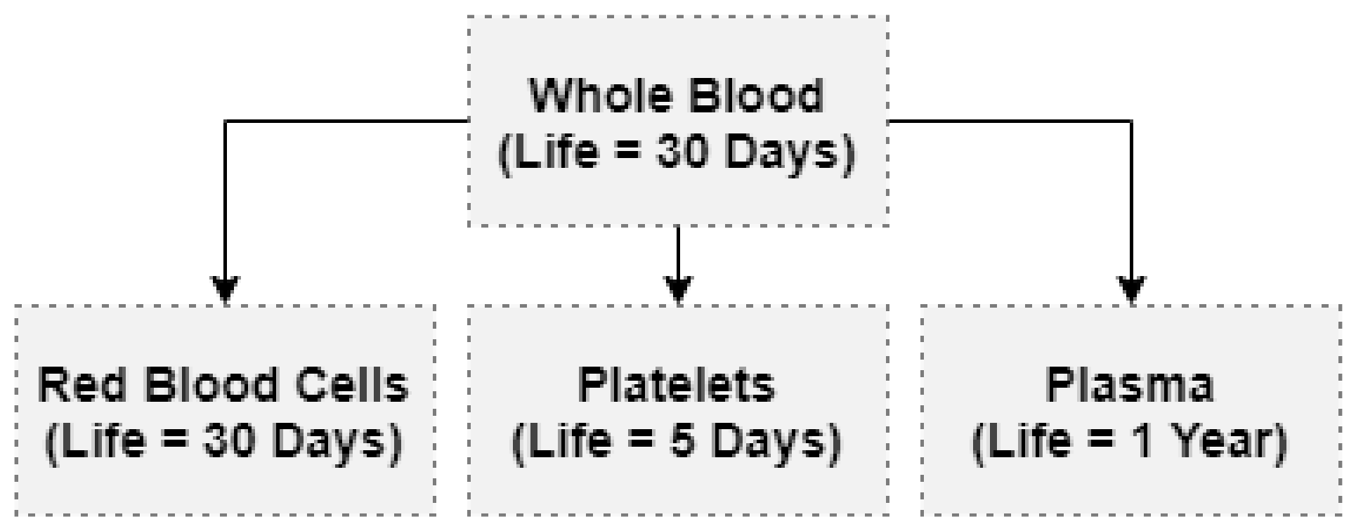
Either a blood processing center or a stockholding facility stores blood products. Platelets must be agitated at a moderate temperature for no more than five days. Blood that will be stored as whole blood is collected in single bags [13]. Blood is collected for componentization based on the number of components required. After componentization, Red Blood Cells (RBCs), Platelets, and Plasma are the three primary components of whole blood (Figure 2). Some blood banks separate from plasma fractionation a fourth component known as cryoprecipitate, which contains a high concentration of clotting factors and is vital for patients with bleeding disorders such as Hemophilia [14].

Figure 2.
Componentizing of whole blood.
2.4. Distribution
This echelon is responsible for the processing of blood product orders as well as the transportation of such orders to the hospitals. Due to blood compatibility and possible restricted inventory, decisions about dates and blood types of delivered components are manufactured. In general, distributing blood between hospitals is essential in order to avoid out dating. In the case that a hospital has a critical need for a specific blood type, they may use blood from a different facility with the earliest date of decay to minimize wastage of blood units.
3. Literature Review
There have been a few studies that have applied time series forecasting methods and machine learning algorithms to predict blood demand at blood bank centers and healthcare facilities. Fortsch et al. [15] evaluated demand forecasting of blood supplies at the New York City Blood Center in 2016, and the best approach for prediction was identified using several forecasting models. The study relied on daily demand data from a blood center from 2006 to 2012. The results indicated that the Autoregressive Moving Average (ARMA) models were more accurate compared to the VARMA models. For the prediction of blood donor arrivals, Lowalekar et al. [16] used an approach based on a theory of constraints TOC. The response to planned donation appointments is the dependent variable, and numerous explanatory variables are used. Among the 18 explanatory variables, they found that several parameters, such as the donor’s age and the number of prior contributions, had an effect on the arrival of donors.
Another study looked at the ability to estimate future blood demand using a neural network (ANN). Fanoodi et al. [17] compared the accuracy of predicting platelet demand based on artificial neural networks (ANN) and ARIMA models. Khaldi et al. [18] presented a case study of using Artificial Neural Networks (ANNs) to forecast future demand for multiple blood components: RBC, plasma, and platelets. Shi Rajendran [19] proposed a model based on time series and machine learning algorithms for anticipating the availability of blood components at blood centers to assist healthcare management in more efficiently managing blood inventory control, thereby minimizing blood shortages and wastage. When the authors compared various strategies, they discovered that time series prediction methods outperformed machine learning algorithms. The Exponential Smoothing Models (ESM) and Autoregressive Integrated Moving Average models (ARIMA), in particular, had the lowest error measures. Incorporating a hybrid demand forecasting model based on statistical time-series modeling, machine learning, and operations research into the development of a demand decision strategy for RBCs, Li et al. [7] proposed a decision integration technique for short-term demand forecasting. The results demonstrated that the proposed strategy can reduce inventory levels by 40% and order frequency by 60%, which may effectively minimize shortages and expiration-related waste.
According to Twumasi and Twumas [20], the effect of data cleansing on the predictive power of models may make time series prediction difficult. Therefore, it has been suggested to use machine learning models such as K-Nearest Neighbor (KNN) regression, General Regression Neural Network (GRNN), and Automatic Regression Neural Network (NNAR) to predict blood demand from a Ghana government hospital with missing values and outliers.
Salazar-Concha and Ramrez-Correa [21] concentrated on forecasting supply by determining the intentions of existing donors regarding future contributions. Under the COVID-19 pandemic’s constrained social interaction framework, Shokouhifar and Ranjbarimesan [22] propose a multivariate time-series deep learning model based on long short-term memory to estimate blood donation and demand and handle the uncertainties occurring during the COVID-19 pandemic. Moreover, new machine learning models based on soft decision-making, such as FPFS-CMC and FPFS-AC, can be used to predict blood demand [23,24].
3.1. Systems Review and Example
A number of blood bank management software programs have been developed in various countries.
3.1.1. Online Blood Donation Reservation and Management System (Saudi Arabia)
Hashim et al. [25] propose a blood-donation management system. The system targets blood donors, blood recipients, and hospitals that act as intermediaries between donors and recipients. The proposed solution allows users to easily access blood bank information (blood type and blood distribution in different hospitals in Jeddah according to the needs of the hospital). The system improves blood bank operations by reducing human error and making hospital-specific distribution easier.
3.1.2. BBIS: Blood Bank Information System Based on Cloud Computing (Indonesia)
Ramadhan et al. [26] proposed a linking system that integrates Indonesian society who can be personal donors as a solution to ensure blood supply availability. By using a web-based and mobile application with cloud computing technology, they suggested a connecting system that integrates Indonesian society, where individuals can be personal donors to keep blood supplies available. The system’s purpose is to make it simpler to find persons who may be donors without consideration to whether the patient is in an emergency condition or not. BBIS offers a bunch of features to facilitate the management of donations (requesting blood applications, managing data on medical histories, donor registration, etc.).
3.1.3. BBMS: Blood Bank Management System (Malaysia)
BBMS is a web-based system that helps blood banks manage blood bags. It was designed for Sultanah Nur Zahirah Hospital in Malaysia (HSNZ) [27]. Each bag’s blood test results can be entered. Based on Inception, Elaboration, Construction, and Transition, test results indicate whether the blood bag can be delivered to the patient. BBMS provides reports such as the blood stock report, donor information, and total blood donation to make blood bank stock more systematic and manageable. When a donor makes a donation, the system may also provide information about the donor’s blood test results.
3.1.4. Blood System in Australia: National Blood Authority (Australia)
In order to provide a safe blood supply to all Australians, the National Blood Authority (NBA) operates a range of information and communication technology (ICT) software programs: the Australian Bleeding Disorders Registry ABDR, BloodPortal, BloodNet, Jurisdictional Reports, MyABDR, and BloodSTAR. It is available 24 hours a day, seven days a week, from the Health Provider Engagement team. These software products provide data to the NBA at various points in the supply chain, from donor management (not directly accessible to the NBA) to inventory, emissions, orders, authorization, product output, results, costs, contract performance, and overall NBA performance [28].
4. Blood Donation and Transfusion Service in Developing Countries: A Case Study of Algeria
4.1. Blood Management Structures
In general, public health facilities collect blood in accordance with the required standards for transfusion activity. These structures are responsible for collecting, separating, controlling, preserving, and distributing blood and its derivatives. For example, in Algeria, there is a coordinated and centralized system with the National Blood Agency, which includes 23 blood transfusion centers in various cities and 217 blood transfusion stations. The agency has a scientific advisory council that is in charge of ensuring a public service mission in terms of monitoring and implementing the national blood policy, as well as promoting blood donation and adhering to good blood-use practices [29].
4.2. Ethical Aspects Related to the Rights of Blood Donors
In the section on the rights of blood donors, the Algerian code of bioethics says:
- A medical interview with the donor must come before the blood donation, as required by medical rules. The donor must also be informed about the blood donation before and during the blood collection.
- The blood donor must be eighteen (18) years old, at least, and sixty-five (65) years old, at the most. However, blood samples can be taken at any age for therapeutic or diagnostic reasons.
4.3. Blood Donor Testing
4.3.1. Blood Screening Tests
Blood donations are systematically tested for HBs, HCV, HIV, and syphilis [29]. The most widely used technology is an enzyme immunoassay (ELISA). For HCV and HIV1, as well as two combinations, antibody and antigen detection kits were used [30].
4.3.2. Screening for Immuno-Hematologic Markers
The ABO-D grouping is performed on all blood donations, and if necessary, the Rhesus Kell phenotype is identified. The search for irregular agglutinins is conducted in all transfusion centers using locally produced and imported erythrocyte panels.
4.4. Component Preparation
Plastic bags are widely used in basically all facilities. CPD-A and SAG-Mannitol bags are both utilized. In practice, nearly all the blood bags collected are sorted into a labile blood product. Platelet apheresis account for 2%, 1%, and <1% of total donations. RBC filtration is performed prior to storage on forty percent of all collected samples [31].
4.5. Transfusion and Transfusion Safety
The establishment, suspension, and modification of blood transfusion facilities, blood transfusion stations, and blood banks may only be decided by the Algerian Ministry of Health and Population on the basis of a proposal from the National Blood Agency [29]. The 24 May 1998 ordinance ensures the safety of distributed blood products:
- After confirming the ABO–RhD blood group compatibility, the phenotype of units to be transfused, and the recipient, a compatibility test must be performed prior to the distribution of whole blood or Red Cell Concentrates (RCC).
- The transfer of blood and perishable products within and beyond the structure responsible for blood transfusion is governed by prescribed procedures: the mode of transport must be chosen based on compliance with safety standards, conservation conditions, and timeliness.
- Blood products must be administered to the intended patients within one hour; otherwise, they must be stored in accordance with storage conditions [29].
4.6. Clinical Uses of Blood Components
Blood transfusion is a medical treatment that must be performed under the supervision of the prescribing physician. Pre-transfusion testing is required. Whether a compatibility test has been performed in the laboratory or not, it must be done in a methodical manner. Primary cross-compatibility tests in indirect combs are routinely performed for many transfusions. Any transfusion-related adverse effects should be notified to the delivery structure [29].
5. Smart Platform for Data Blood Bank Management
The goal is to design and build a smart blood bank information system that will improve supply chain performance and deal with uncertain demand using machine learning.
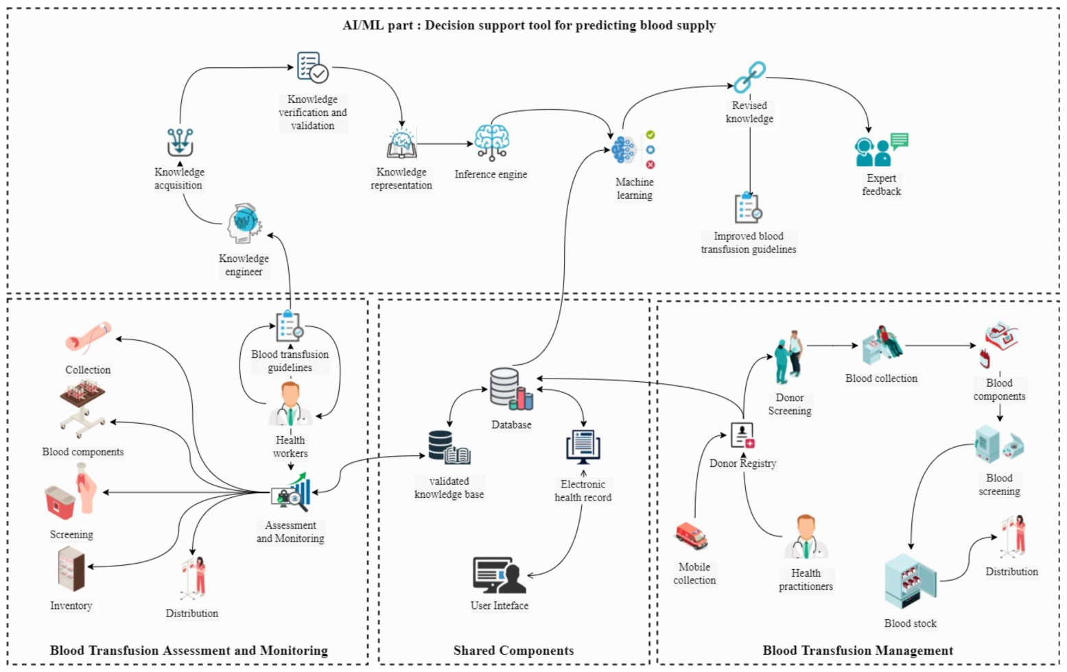
As shown in Figure 3, the framework consists of four subsystems: (1) Managing blood transfusions from fixed and mobile blood collection centers, including the registration of donor information, tests, and all the information required to trace the blood supply chain from collection to distribution and exploitation. (2) The Blood Transfusion Evaluation and Monitoring Subsystem, whose purpose is to facilitate the monitoring of the most crucial stages of blood management due to the vast amount of data collected during each transfusion. (3) An AI-ML decision support tool for forecasting blood demand, predicting blood donor behavior, and identifying return donors, which includes a system for acquiring knowledge after its validation by experts in the field of health and a knowledge engineer who collects and represents the information to be exploited later by the adaptive learning system. All bases discovered by machine learning techniques using previously collected blood chain supply information in the database are then evaluated by experts so that their input and consent can be used to improve the validated knowledge base.
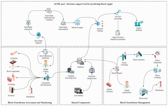
Figure 3.
System architecture.
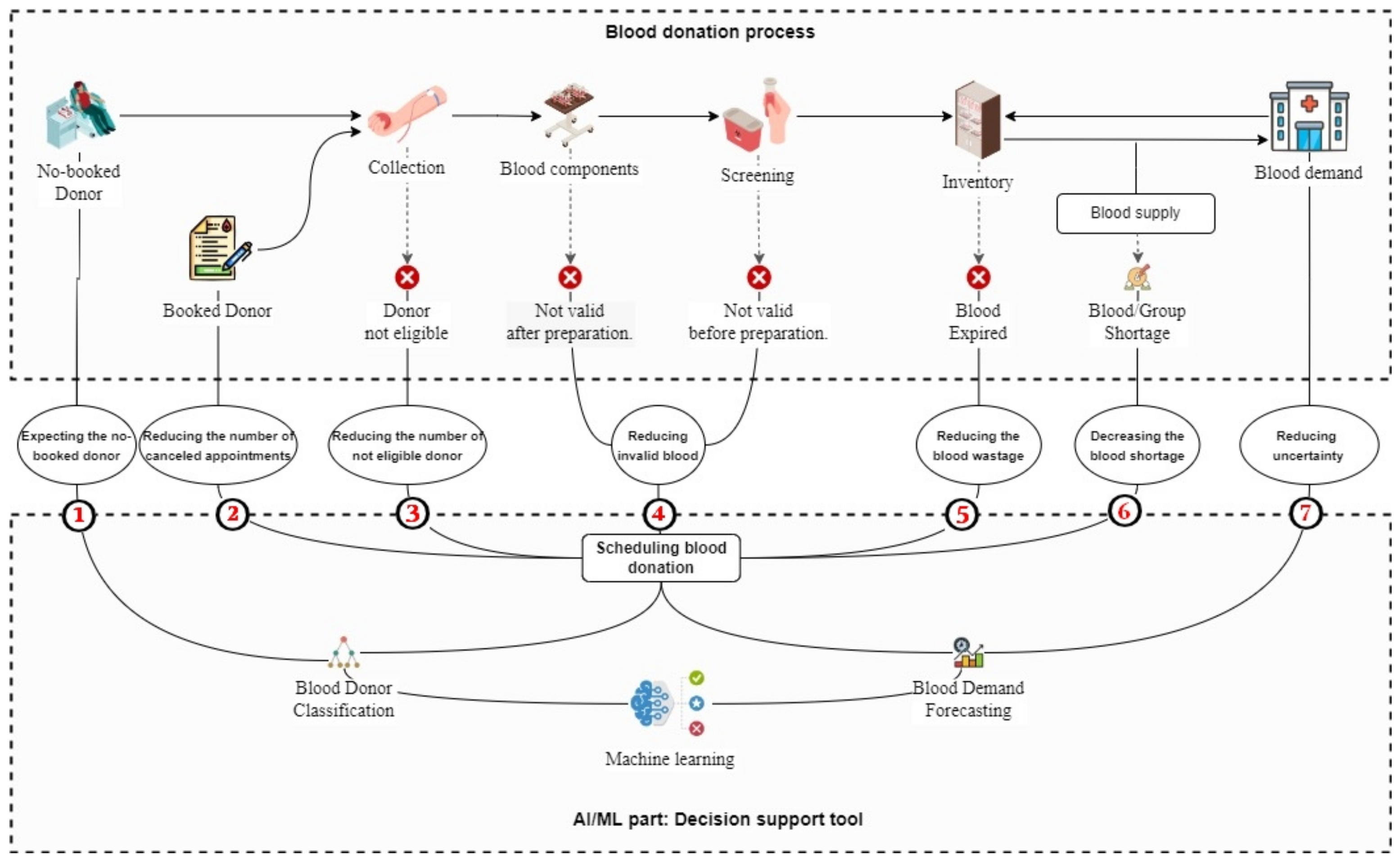
The system directly and indirectly improves all stages of blood supply (see Figure 4), classifying blood donor aids in the prediction of daily unbooked donors, which helps control the amount of blood collected while also improving working conditions for health workers and reducing long donation lines (1). Scheduling blood donations with consideration of the predicted number/type of blood required and selecting suitable donors will help improve blood volumes by reducing the number of canceled appointments (2) by blood donor classifiers and improving quality by carefully scheduling donors, which will help reduce the number of unqualified donors (3) and indirectly reduce invalid blood after and before preparation (4). Balancing blood collection and demand may help to reduce uncertainty (7). As a result of the aforementioned enhancements, both the quantity of blood wasted (5) and the blood shortage can be reduced (6).
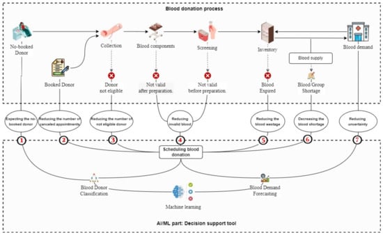
Figure 4.
Flow diagram of the proposed system.
6. Materials and Methods
As mentioned earlier, the aim of the work is to create effective prediction methods for whole blood demand forecasting using time series prediction methods and machine learning algorithms, and to predict blood donor behavior to identify return donors. In this section, we describe some database characteristics used in this work as well as discuss the various models used to develop the proposed solution, along with a brief summary. Then we explore some econometric analyses and the underlying assumptions used to calculate the stationarity and normality of the data.
6.1. Data Collection
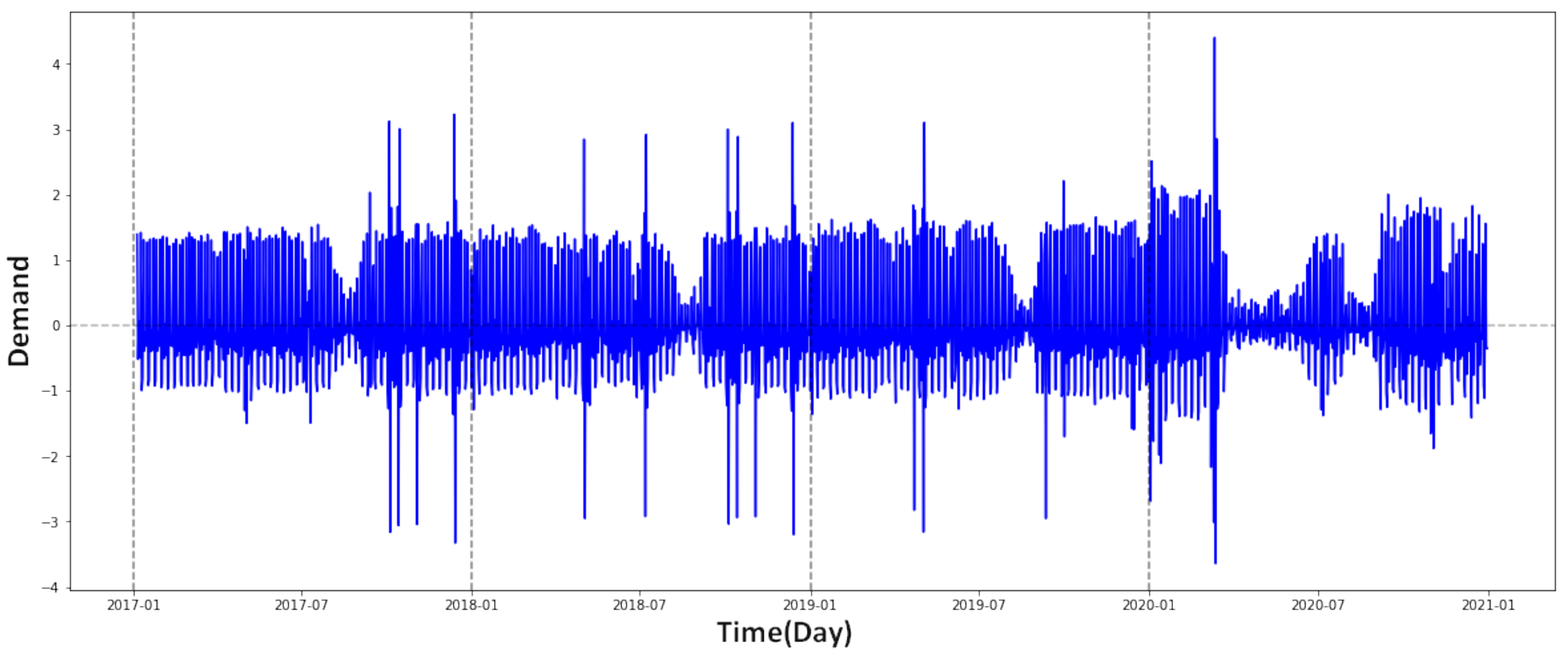
The data used in this work were obtained from the National Blood Agency in Algeria. We used data on the total blood demand of hospitals and health services in Algiers Province, Algeria, due to two factors: first, the capital city has a large blood supply chain. Second, data was lacking in other places, and some blood facilities did not have data for the study’s time period. Health records were used to collect historical supply data for the four-year period from 2017 to 2021. The data were analyzed using Python data science libraries to extract daily blood supply (Figure 5 and Table 1) and donor information during the previously mentioned time period (1461 consecutive days).
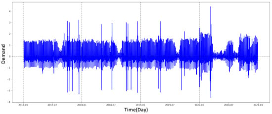
Figure 5.
Daily whole blood donations, 2017–2021 (normalized data).

Table 1.
The 2017–2020 weekly blood supply statistics.
Table 1 shows that for each year, the average weekday blood supply remains almost constant, with a marked decrease over the last two years. This is due to the COVID-19 pandemic. However, we can see that the blood supply is very high on Monday, Tuesday, and Wednesday, and is relatively high on Thursday and Sunday. Friday and Saturday supplies are significantly lower, due to the weekend days in Algeria.
The data on blood donors includes the date of each donor’s first donation and the dates of all subsequent donations during the study period. Table 2 presents the dataset attribute descriptions. However, donors who donated once for the first time in 2021 were excluded from the analysis to ensure that all first-time donors had at least one year to make a second donation. The selection of a 1-year follow-up period is based on the fact that first-time donors returned, on average, after 14 months. Among the remaining 2565 donors, 1014 donors were return-donors and 1551 were non-return donors. Table 3 summarizes some statistics of the blood donors dataset by blood group type , such as the number of donors by gender and class (return donors, non-return donors). The table also shows the average of the following statistics: months since last donation (Recency), total number of donations (Frequency), amount of blood donated (Monetary), months since first donation (Time), and total number of rejected donations (Rejected).

Table 2.
Dataset attributes of blood donor.

Table 3.
Descriptive statistics of the blood donors data.
6.2. Time Series Forecasting Models
This section describes the different time series forecasting models used in this work, including the AutorRgressive model, ARMA model, ARIMA model, Seasonal ARIMA model, Seasonal Exponential Smoothing model, and the Multiplicative Holt–Winters model.
6.2.1. Autoregressive (AutoReg) Model
The AutorRgressive method predicts linear regression models for data with errors that are automatically associated or heterogeneous. It is a valuable tool for forecasting, since it generates anticipated values by combining the time series and systematic parts of the model. In creating predictions, the autoregressive error model considers recent deviations from the trend. Following that, the AutoReg model regresses the series value from time t on the series values at times . The mathematical formula is expressed as follows [32]:
where is the forecasting value at time t, are the linear regression coefficients, and is the random error variable (It is commonly assumed that the distribution is normal, with a mean of zero and variance ).
6.2.2. Autoregressive Moving Average (ARMA) Models
The most common time series models in statistics are ARMA models (Autoreg Ressive Moving Average). Given a time series , the ARMA model is a method to forecasts the future values of this series. The model is composed of two parts: AR and MA, autoregressive and a moving average, respectively. The model is generally denoted ARMA (p,q), where p is the order of the AR part and q is the order of the MA part. An autoregressive model of order p, abbreviated AR (p), is written:
where are the model parameters, c is a constant, and is white noise. The constant is often omitted in the literature, with the process then being said to be centered.
Additional constraints on the parameters are necessary to guarantee stationarity. For example, for AR (1) model, processes such as are not stationary.
An autoregressive moving-average model of orders (p,q) is a discrete temporal process verifying:
where the and are the model parameters and the error terms .
6.2.3. Autoregressive Integrated Moving Average (ARIMA) Model
The ARIMA model is made popular by Box–Jenkins models [18].
The “I” in the ARIMA model stands for “integrated” for integration. By differentiating the time series, it is possible to remove the trends they present in order to stationarize them.
The correction of a non-stationarity in terms of variance can be carried out by transformations of the logarithmic type (if the variance increases with time) or conversely exponential. These transformations must be carried out before differentiation. The fundamental process that creates the time series model is as follows:
t represent the index of time, the time series , and C is the backward shift operator.
The ARIMA model is therefore a combination of this differentiation process and the classical ARMA process.
6.2.4. Seasonal ARIMA Model (SARIMA)
So far, we have focused on non-seasonal data and non-seasonal ARIMA models. ARIMA models, on the other hand, can model a wide range of seasonal data. A seasonal ARIMA model is formed by including additional seasonal terms in ARIMA models. It is written as follows:
where s is the duration of the seasonal cycle, D is the order of the seasonal differencing, and Q is the order of the seasonal moving average process. Uppercase notation is used for seasonal parts of the model, and lowercase notation is used for non-seasonal elements of the model. The seasonal component of the model consists of words that are comparable to the non-seasonal components of the model but include seasonal period backshifts.
is dependent to time series at time t, with mathematical formula:
where is the constant mean, is the seasonal backward shift operator, is the seasonal moving-average component, and is the seasonal autoregressive component.
For quarterly data , an model (without a constant) can be written as:
The additional seasonal terms are multiplied by the non-seasonal terms.
6.2.5. Seasonal Exponential Smoothing Model (SESM)
The following equation gives the predicted value at time :
The smoothing equations and are as follows:
where is a given observation at time t, and are the level and seasonal smoothing parameters, respectively, is the estimated level component at time t, and the times after which the seasonal cycle denoted by p.
6.2.6. Multiplicative Holt–Winters Model
Holt (1957) and Winters (1960) extended Holt’s method to capture seasonality. Winter extended Holt’s method by using exponential smoothing to update seasonality indices.
The Holt–Winters model, commonly known as triple exponential smoothing, smoothes time series data using three forms of exponential smoothing: value, trend, and seasonality. The following Equation (10) provides the forecast at time for a time series with a trend T, level estimates , and a constant seasonal component using the Holt–Winters model:
The forecast at time for a time series with a trend T is provided by the following equation:
The smoothing equations are obtained using the following formula:
and represent the level and trend, respectively; the seasonal corresponding constants c, is the estimated level at time t, and is a given observation at time t.
6.3. Machine Learning Algorithms
This section discusses the most important machine learning algorithms that adapt to the time series employed in this work, which are as follows: Artificial Neural Networks (ANN), Recurrent Neural Networks (RNN), Linear Regression (LR), and Support Vector Regression (SVR). Table 4 compares the characteristics of various learning techniques according to seven criteria, which are as follows: (1) accuracy in general, (2) learning speed, (3) speed of classification, (4) tolerance to highly interdependent attributes, (5) tolerance to noise, (6) dealing with the danger of overfitting, and (7) model parameter handling.

Table 4.
Comparing machine learning algorithms (**** stars represent the best performance and * stars represent the worst).
6.3.1. Artificial Neural Networks (ANN)
It is a non-hypothetical, data-driven technique, and neural networks have proven to be a contemporary and reliable solution to the prediction of complex functions. An artificial neural network (ANN) consists of a network of limited processing elements called neurons. The neuron’s role is to receive inputs, process them, and give output signals. A network is composed of a row of neurons from a layer, as well as multiple layers connected together.
To build an artificial neural network, we must first define a set of input variables before using trial and error to find the best-predicted network design. A multi-layer perceptron neural network is employed in this work, where p represents the number of inputs, n defines the number of neurons in each layer, f represents the activation function, a denotes the output of each layer, the bias is b, and w represents the vectors of weights.
6.3.2. Recurrent Neural Network (RNN)
A basic RNN is made up of three layers: the input layer, a hidden layer with frequent connections (context layer), and the output layer. RNN can be described using deterministic transitions between states (from the past to the current hidden state ):
An RNN can presented by the following equation:
where f ∈ {sigm, tanh}.
6.3.3. Linear Regression (LR)
A linear regression model is a regression model that attempts to create a linear relationship between an explained variable and one or more explanatory factors. The linear regression model, in general, indicates a model in which the conditional expectation of y a given x is an affine function of the parameters. However, we can also examine models in which it is the conditional median of y knowing x or any quantile of the y knowing the x distribution that is an affine function of the parameters.
We consider the model for a single i. For each individual, the explained variable is written as a linear function of the explanatory variables:
where and are constants and represents the error.
A simple linear model is a linear regression model with one explained variable. This model is often presented in statistical academic books, under the title of fine-tuning. As a result, we have two random variables, an explained variable Y (a scalar), and an explanatory variable X (also a scalar). There are n realizations for these variables.
6.3.4. Support Vector Regression (SVR)
Machine learning is well known for its ability to handle high-dimensional data. SVR is founded on the framework of statistical learning theory, and as a result of this mathematical foundation, it provides a rational solution to machine learning challenges. Assuming that a set of m training samples , where represent the input example and is the forecasting value for . is the vector of observed values.
The goal of SVR is to approximate the regression function :
where w is the regression vector and b is a scalar value.
6.4. Evaluating Forecasting Models
We apply three distinct forecast error measures to evaluate model performance and method accuracy: Mean Absolute Error (MAE), Mean Squared Error (MSE), Mean Absolute Percentage Error (MAPE).
If we suppose that , represents historical data and are the data we aim to forecast, and then n values of forecast errors, , where . Table 5 summarizes the three evaluation methods of forecasting models performed in this work.

Table 5.
The three evaluation methods of forecasting models performed used.
6.5. Econometric Analysis and Assumptions
This section discusses some econometric analyses and the normality of the data. It goes through a data stationary test as well as one of the Box–Jenkins methodology hypotheses for data normality. Table 6 summarizes several of the common economic tests and procedures used in this work. We use the table because it is easy to understand and describes each test in a clear way.

Table 6.
Econometric tests and procedures.
6.5.1. Stationarity of the Data
As previously noted in Table 1, the demand for blood differs by day of the week, with demand being highest on Monday, Wednesday, and Tuesday and lowest on other days, as expected. Daily demand statistics may occasionally reveal an unstable pattern due to the variation of blood that is not consistent on each day of the week. This pattern of week-to-week unpredictability affects forecasting. Furthermore, analysis reveals that weekly demand data includes several auto-correlated periods, increasing the non-stationarity of demand even further and making it unpredictable to estimate blood needs over a longer time horizon. The issue of non-stationarity must be addressed before applying forecasting models. However, for high prediction accuracy, this is required. The ARMA model is based on the assumption that the variability pattern in the data is reasonably consistent (i.e., stationarity), to reduce prediction errors, it employs an adaptive technique to construct a forecasting model based on random demand patterns.
ACF and PACF charts were utilized to examine reversibility and identify the type and order of the model for time series data. As depicted in Figure 6, the ACF and PACF charts exhibit an exponential or oscillating trend that converges to zero. This suggests that the series is reversible and the predicted values are credible.

Figure 6.
The ACF and PACF plots for total blood demand data.
We examined numerous combinations of MA and AR lags to determine whether or not this assertion was accurate. The graphs (Figure 6) indicate that the lags considered for the TBD exhibit a decreasing trend from 12 to 8 lags. The Augmented Dickey–Fuller test (see Table 6 and Table 7) for data stationarity validated the results.

Table 7.
Augmented Dickey–Fuller test for Total Blood Demand. Decision: (T-statistics > Critical values).
6.5.2. Normality of the Data
Data normality is another assumption of the Box–Jenkins method. To determine whether a probability distribution corresponds to a normal distribution (see Table 6), the total blood demand was subjected to the Jarque–Bera test, which analyzes skewness and kurtosis values. The Jarque-Bera test results are shown in Table 8. The test statistic is 41.54 and the corresponding p-value is 9.51, as can be seen. Since this p-value is greater than 0.05, the null hypothesis is not rejected. We have sufficient evidence to conclude that the skewness and kurtosis of these data are consistent with a normal distribution.

Table 8.
Jarque–Bera test for normality of data.
7. Results and Experimentation
In this section, we present the results obtained for both blood demand forecasting using time series models and machine learning algorithms for case study data and prediction of blood donor behavior by identifying return donors using machine learning models such as: Artificial Neural Network, Logistic Regression, Support Vector Machines, Decision Trees, Random Forest, and Naive Bayes.
Table 9 displays the accuracy measures for the six time series models discussed in Section 6.2. AutoREG model, ARMA model, and ARIMA model generate minimal error measures through their results. We conclude that these three time series models provide the most accurate blood supply prediction. The performance of the machine learning algorithms discussed in Section 6.3 are summarized in Table 10. We notice that ANN, LR, and SVR models generate the lowest error measures. We conclude that these three machine learning models offer the most accurate blood supply prediction.

Table 9.
Error measures obtained under the six time series models.

Table 10.
Performance of machine learning algorithms (statistics of fit).
For the classification task aimed at predicting donor return, implementation was carried with the six classifiers were generated: Artificial Neural Network, Logistic Regression, Support Vector Machines, Decision Trees, Random Forest and Naive Bayes, and K-Nearest Neighbor.
The test results for the six models are presented in Table 11. Low recall of Naive Bayes, logistic regression, and support vector machines (65%) indicated that the models were suffering from an unrecognized positive category; that is, many returning donors were predicted as non-returning donors. On the other hand, calling ANN (95%) and Random Forest (94%) was higher, indicating that two models were better than LR (65%), SVM (64%), DT (62%), and Naive Bayes (62%) in correctly predicting the minority positive category (returning donor).

Table 11.
Test results for the six classifiers for prediction of donors return.
Table 12 represents experimental results of blood supply forecasting using the best-performing models from machine learning (ANN, LR, and SVR) and time series methods (AutoREG, ARMA model, and the ARIMA model).

Table 12.
Blood supply predictions using the best performing methods (time series and machine learning models).
8. Discussion
As mentioned in the previous section, the results in Table 9 and Table 10 showed that six models provided the best and most accurate results in terms of learning accuracy and predictive efficacy, three of these models are AUTOREG, ARMA, and ARIMA, which represent time series methods, and three models are ANN, LR, and SVR, which represent artificial intelligence methods. Although autoregressive approaches are linear, they outperformed machine learning models in the first two months, as shown in Table 12. Thereafter, the accuracy of the time series models declined, while the prediction accuracy of the machine learning models, particularly the ANN model and SVR model, improved gradually.
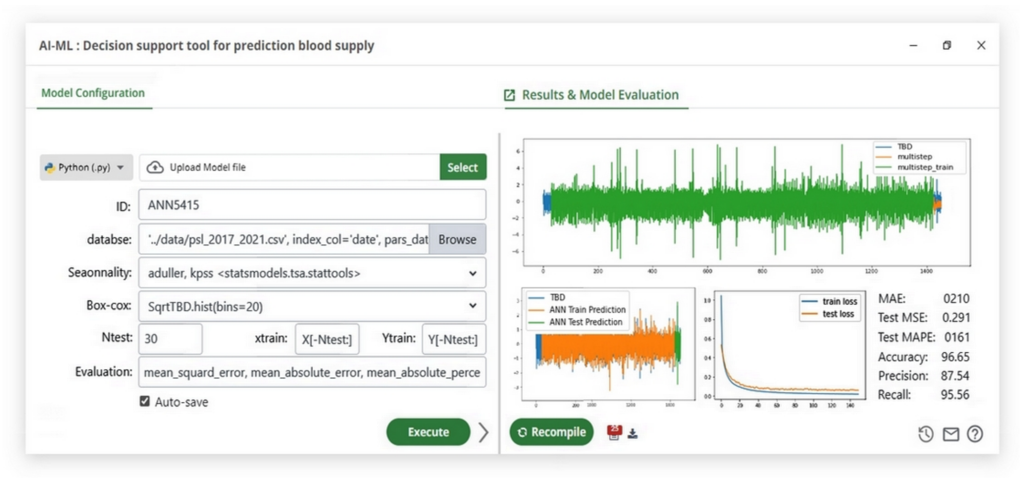
In fact, one of the primary reasons that machine learning approaches provide more accurate predictions than linear models is that artificial neural networks and SVR can simulate the dynamic interaction with many variables in the same period, thereby limiting the ability to be directly affected by previous data trends. When the prediction results of the proposed solution models are compared to the classical statistical methods used in traditional blood bank management systems, it is obvious that there is a significant difference in prediction accuracy of more than 30% (Table 12), making the proposed blood donation management platform (see Figure 7) more effective compared to the classic methods used before.

Figure 7.
AI/ML module configuration overview and run results execution.
9. The Impact of the Proposed Solution on the Results of the Case Study
We put a test version of the proposed system into place at one of the largest blood donation centers in Algiers so we could see how well it worked.
During about a year (from March to December 2021) of experimental work, no serious technical problems were encountered; if we exclude the monthly support request, technical support and service requests can be categorized as follows: (1) technical training and guidance, (2) abnormal data or inconsistent information, and (3) archive and migration of the previous data to review it in the system. Most of which were obviously related to the nature of the user and the lack of training in the use of information technologies.
In this section, we present several graphs and reports gathered during the evaluation period to determine the impact of the proposed system on the blood bank’s management. The following phases of the blood supply system are presented: blood collection, testing, blood processing, and distribution.
The difference between the test year and the previous year is not taken into account in the comparative analysis of the results because the previous year’s blood product statistics were significantly impacted by the COVID-19 pandemic [22,36]. Therefore, in this study, we suggest comparing the results of 2021, which represents the experimental period, with the average of the previous five years (2015–2020).
9.1. Blood Collection Reports
In this section, we display more details and statistics about the total number of blood bags collected (whole blood and apheresis) within a specified period of time and over a specified number of years. This result is useful for administrators to know the number of blood bags collected and the types of collections, which they can then compare to previous years’ results to study the impact of the proposed system on increasing the quantity and quality of blood collection; see Figure 8 and Figure 9.
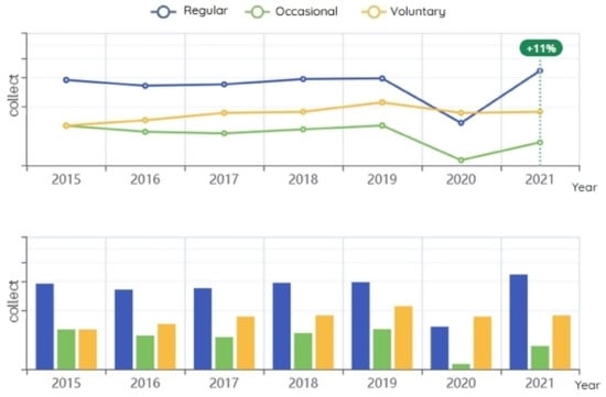
Figure 8.
Blood collected per year (whole blood and apheresis).
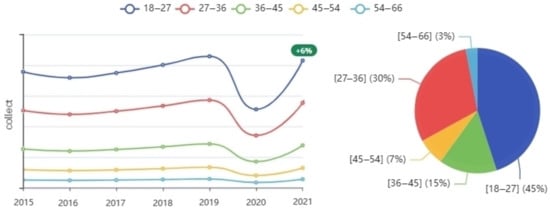
Figure 9.
Number of donations by age group per year.
Figure 8 displays the total number of blood bags collected by donor type: regular, occasional, and voluntary donors. A regular donor is a donor registered in the database as a periodic donor, meaning that they donated more than once according to the specified period since their last donation; most of the time, they are in good health and able to donate on a regular basis. Occasional donors regularly donate at blood collection and awareness events (places of worship, universities, etc.) and are mostly collected through mobile blood collection sites. Voluntary donors donate to help a specific patient or patients; most of the time, they are family members of the patient. The results show that the use of the proposed system improved collected blood volumes by 11% compared to the average of the previous five years. The highest improvement was in the amount of blood collected from regular donors (Figure 8). This is expected, because the decision support tool was designed to study the behavior of donors based on the data of previous donors, who are often regular donors.
The following graph (Figure 9), represents blood donations by age group in each year. As we note, most of the donors are of a young age group (between 18 and 36 years old). We notice an increase of seven percent in the number of donors obtained from donors aged 18 to 36 years, with a slight decline for the rest of the ages, and this is directly due to the quality of the stored data as well as the specific goals during donor scheduling so that the system proposes an appointment schedule aiming to increase the number of donors by reducing the number of cancellations and at the same time improving blood quality through targeted selection of donors during the scheduling of appointments. The information extracted may greatly help health specialists determine the best target age group. The reason is also that young people are more likely to be healthy in general and, therefore, to donate blood well. Since the system is primarily based on scheduling donation appointments in fixed blood centers based on previous donor data, the graph demonstrates a significant increase of more than 15% in the amounts of blood collected at the level of the fixed blood center, which is directly correlated with the improvement goals.
9.2. Blood Component Reports
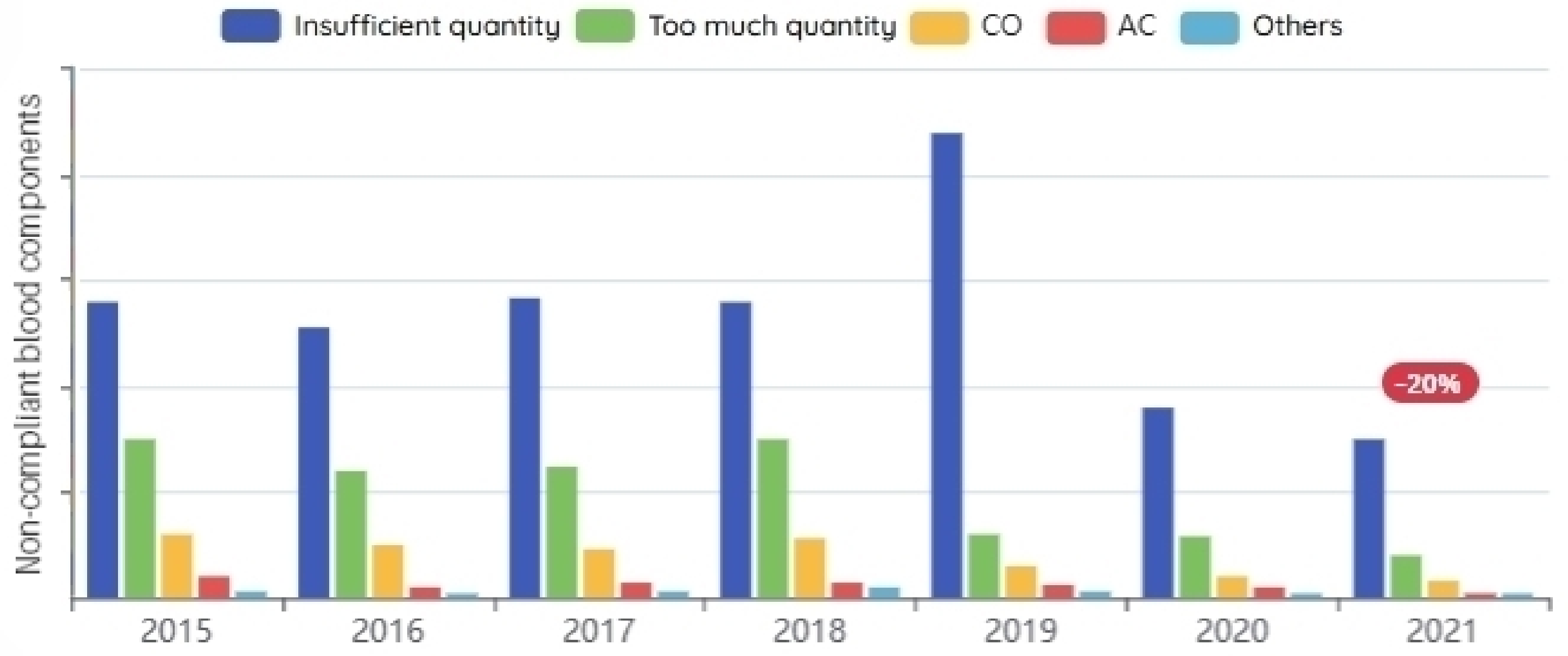
The preparation of blood components necessitates adherence to a strict health standard, and the quantities of components extracted from the blood must meet specific requirements both after and before the preparation. A series of tests and treatments are performed on blood components to reduce the risk of pathogen transmission during the blood transfusion. Blood components that did not meet the required standards before or after blood preparation are depicted in Figure 10.
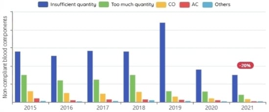
Figure 10.
Non-compliant blood components before/after preparation per year.
Any blood donation center must expand the categories of blood donors in order to ensure production continuity and increase quantity. It receives new donors on a daily basis, which helps improve the database. We observed that concentrating on increasing the number of regular donors had a positive effect on the percentages of unusable blood, because the less the reliance on the cause of occasional donors, the less non-compliant blood components before/after preparation. This significantly improves the efficiency of blood bank management by lowering the proportions of unusable blood, as shown in Figure 10.
9.3. Blood Testing Reports
The screening tests carried out in the biological qualification laboratories for the donation include serological tests (search for specific antibodies directed against an infectious agent or search for antigen) and screening tests for viral genomes.
A serological test detects the syphilis causative agent (Treponema pallidum) on each donation. A donation is compliant as long as all the screening tests are negative. The results of the tests in Figure 11 show a significant decrease in the number of positive cases, and it was for the same reasons as we mentioned earlier: the more we rely on blood donations from healthy regular donors, the more we reduce the number of positive cases of blood-borne diseases.
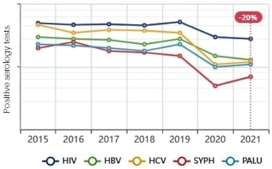
Figure 11.
Positive infectious serology.
9.4. Inventory and Distribution Reports
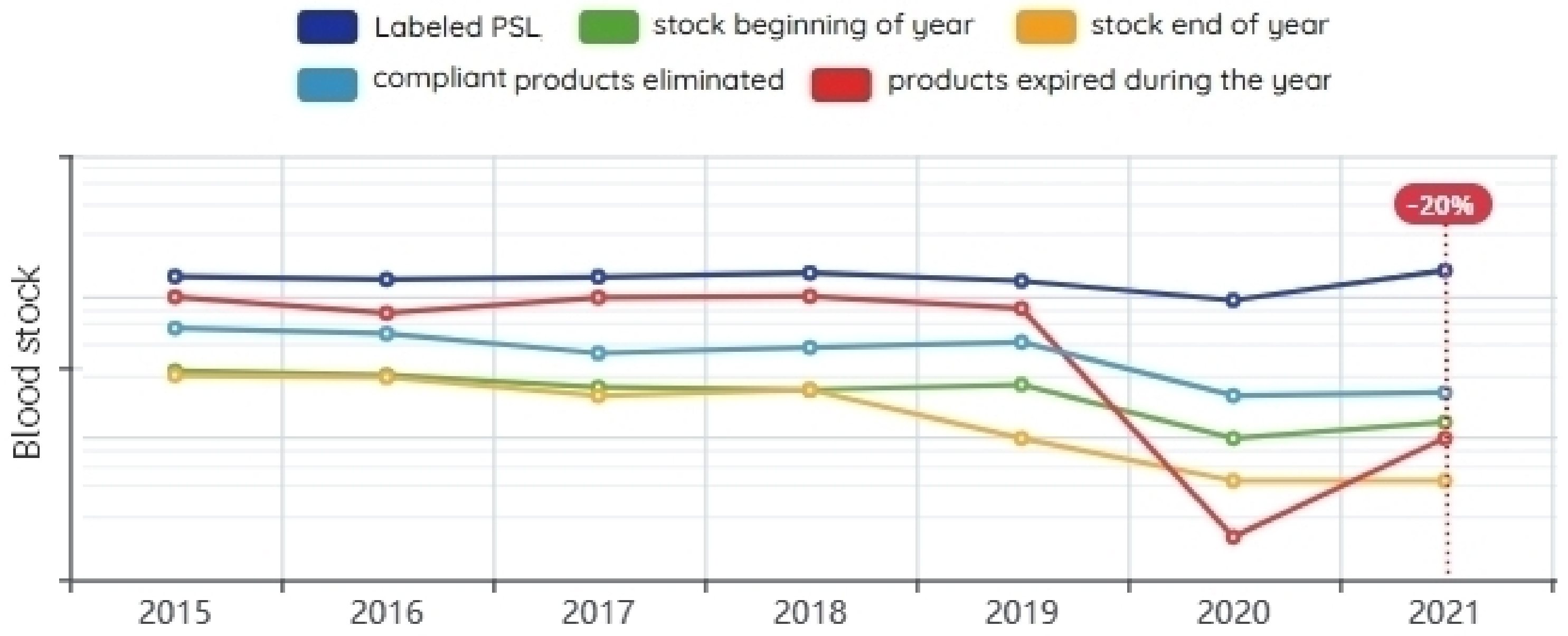
In this section, we present a graphical representation of the amount of blood available in the blood store by the type of component required. It is also possible through the blood transfusion assessment and monitoring module to show the rest of the blood stock from last year, statistics comparing the amount of blood that was stored with the amount of blood distributed, display the percentage of expired blood, and calculate the wastage of blood (Figure 12).
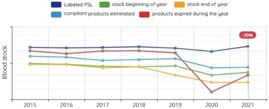
Figure 12.
Blood inventory statistics.
The results of previous years showed that the more blood collected, the more blood was wasted. The lower the proportions of collected blood quantities, on the other hand, the greater the blood shortage. In the experimental period of the proposed system, we observed an increase in the quantity and quality of collected blood, and the percentage of wasted blood decreased by 20%. Unfortunately, we were not able to extract enough information to calculate the percentage of blood shortage.
10. Conclusions
In this paper, we propose a smart platform for data-driven blood bank management that can reduce blood demand uncertainty by forecasting blood collection and demand, as well as reduce blood wastage and shortage by balancing blood collection and distribution based on effective blood inventory management. This leads to a significant improvement in the quality and quantity of blood collected, with results showing an 11% increase in the percentage of blood collected and a 20% reduction in blood waste. It can potentially reduce the inventory level shortage by balancing blood collection and distribution based on effective blood inventory management and by effectively scheduling blood donation appointments that reduce the number of canceled appointments. The proposed solution has the potential to improve the blood supply chain by foreseeing demand and reducing uncertainty, which in turn, may reduce blood loss and shortages, which may save lives because people die or suffer as a result of a lack of blood products or safe blood transfusions in the world. Among the challenges posed by the proposed system is its direct impact on the quality and quantity of data; consequently, the dataset must be updated whenever new and dependable information becomes available, and forecasting accuracy must be continuously monitored. Therefore, one of the most important things that we focus on in our future work is supporting the system with a module to clean the new data in a way that does not require the presence of a data science expert. In the future, we propose using bio-inspired algorithms, such as genetic algorithms and evolutionary strategies, to optimize the scheduling of blood donation appointments that are convenient for both the bank and the donor.
Author Contributions
Conceptualization, W.B.E., A.H. and B.S.; methodology, W.B.E., A.H. and B.S.; software, W.B.E.; validation, W.B.E. and B.S.; formal analysis W.B.E., A.H. and B.S.; investigation, W.B.E. and B.S.; data curation, W.B.E. and B.S.; writing—original draft preparation, W.B.E., A.H. and B.S.; writing—review and editing, W.B.E. and B.S.; visualization, W.B.E.; supervision, B.S.; project administration, A.H. and B.S. All authors have read and agreed to the published version of the manuscript.
Funding
This research received no external funding.
Data Availability Statement
Some primary data for the study is available on http://www.ans.dz/.
Conflicts of Interest
The authors declare no conflict of interest.
References
- Uthayakumar, R.; Priyan, S. Pharmaceutical supply chain and inventory management strategies: Optimization for a pharmaceutical company and a hospital. Oper. Res. Health Care 2013, 2, 52–64. [Google Scholar] [CrossRef]
- Privett, N.; Gonsalvez, D. The top ten global health supply chain issues: Perspectives from the field. Oper. Res. Health Care 2014, 3, 226–230. [Google Scholar] [CrossRef]
- Fattahi, M.; Mahootchi, M.; Husseini, S. Integrated strategic and tactical supply chain planning with price-sensitive demands. Ann. Oper. Res. 2016, 242, 423–456. [Google Scholar] [CrossRef]
- Addis, B.; Carello, G.; Grosso, A.; Lanzarone, E.; Mattia, S.; Tànfani, E. Handling uncertainty in health care management using the cardinality-constrained approach: Advantages and remarks. Oper. Res. Health Care 2015, 4, 1–4. [Google Scholar] [CrossRef]
- Pierskalla, W. Supply chain management of blood banks. In Operations Research And Health Care; Springer: Boston, MA, USA, 2005; pp. 103–145. [Google Scholar]
- Rajendran, S.; Ravindran, A. Inventory management of platelets along blood supply chain to minimize wastage and shortage. Comput. Ind. Eng. 2019, 130, 714–730. [Google Scholar] [CrossRef]
- Li, N.; Chiang, F.; Down, D.; Heddle, N. A decision integration strategy for short-term demand forecasting and ordering for red blood cell components. Oper. Res. Health Care 2021, 29, 100290. [Google Scholar] [CrossRef]
- Williams, E.; Harper, P.; Gartner, D. Modeling of the collections process in the blood supply chain: A literature review. IISE Trans. Healthc. Syst. Eng. 2020, 10, 200–211. [Google Scholar] [CrossRef]
- Baş Güre, S.; Carello, G.; Lanzarone, E.; Yalçındağ, S. Unaddressed problems and research perspectives in scheduling blood collection from donors. Prod. Plan. Control 2018, 29, 84–90. [Google Scholar] [CrossRef]
- Baş, S.; Carello, G.; Lanzarone, G.; Ocak, Z.; Yalçındağ, S. Management of blood donation system: Literature review and research perspectives. Health Care Syst. Eng. Sci. Pract. 2016, 169, 121–132. [Google Scholar]
- Osorio, A.; Brailsford, S.; Smith, H. A structured review of quantitative models in the blood supply chain: A taxonomic framework for decision-making. Int. J. Prod. Res. 2015, 53, 7191–7212. [Google Scholar] [CrossRef]
- Radcliffe, R.; Bookbinder, L.; Liu, S.; Tomlinson, J.; Cook, V.; Hurcombe, S.; Divers, T. Collection and administration of blood products in horses: Transfusion indications, materials, methods, complications, donor selection, and blood testing. J. Vet. Emerg. Crit. Care 2022, 32, 108–122. [Google Scholar] [CrossRef]
- Gammon, R.; Coberly, E.; Dubey, R.; Jindal, A.; Nalezinski, S.; Varisco, J. Patient Blood Management—It Is about Transfusing Blood Appropriately. Ann. Blood 2022, 7. Available online: https://aob.amegroups.com/article/view/6877 (accessed on 10 October 2022). [CrossRef]
- Standards for Blood Banks and Transfusion Services. Standards for Blood Banks and Transfusion Services; Committee on Standards: Brussels, Belgium; American Association of Blood Banks: Bethesda, MD, USA, 2020.
- Fortsch, S.; Khapalova, E. Reducing uncertainty in demand for blood. Oper. Res. Health Care 2016, 9, 16–28. [Google Scholar] [CrossRef]
- Lowalekar, H.; Ravi, R. Revolutionizing blood bank inventory management using the TOC thinking process: An Indian case study. Int. J. Prod. Econ. 2017, 186, 89–122. [Google Scholar] [CrossRef]
- Fanoodi, B.; Malmir, B.; Jahantigh, F. Reducing demand uncertainty in the platelet supply chain through artificial neural networks and ARIMA models. Comput. Biol. Med. 2019, 113, 103415. [Google Scholar] [CrossRef]
- Khaldi, R.; El Afia, A.; Chiheb, R.; Faizi, R. Artificial neural network based approach for blood demand forecasting: Fez transfusion blood center case study. In Proceedings of the 2nd International Conference on Big Data, Cloud and Applications, Tetouan, Morocco, 29–30 March 2017; pp. 1–6. [Google Scholar]
- Shih, H.; Rajendran, S. Comparison of time series methods and machine learning algorithms for forecasting Taiwan Blood Services Foundation’s blood supply. J. Healthc. Eng. 2019, 2019, 6123745. [Google Scholar] [CrossRef]
- Twumasi, C.; Twumasi, J. Machine learning algorithms for forecasting and backcasting blood demand data with missing values and outliers: A study of Tema General Hospital of Ghana. Int. J. Forecast. 2022, 38, 1258–1277. [Google Scholar] [CrossRef]
- Salazar-Concha, C.; Ramírez-Correa, P. Predicting the Intention to Donate Blood among Blood Donors Using a Decision Tree Algorithm. Symmetry 2021, 13, 1460. [Google Scholar] [CrossRef]
- Shokouhifar, M.; Ranjbarimesan, M. Multivariate time-series blood donation/demand forecasting for resilient supply chain management during COVID-19 pandemic. Clean. Logist. Supply Chain. 2022, 5, 100078. [Google Scholar] [CrossRef]
- Memiş, S.; Enginoğlu, S.; Erkan, U. A classification method in machine learning based on soft decision-making via fuzzy parameterized fuzzy soft matrices. Soft Comput. 2022, 26, 1165–1180. [Google Scholar] [CrossRef]
- Memiş, S.; Enginoğlu, S.; Erkan, U. A new classification method using soft decision-making based on an aggregationoperator of fuzzy parameterized fuzzy soft matrices. Turk. J. Electr. Eng. Comput. Sci. 2022, 30, 871–890. [Google Scholar] [CrossRef]
- Hashim, S.; Al-Madani, A.; Al-Amri, S.; Al-Ghamdi, A.; Nahla, B. Online Blood Donation Reservation And Managementsystem In Jeddah. Life Sci. J. 2014, 11, 60–65. [Google Scholar]
- Ramadhan, M.; Amyus, A.; Fajar, A.; Sfenrianto, S.; Kanz, A.; Mufaqih, M. Blood Bank Information System Based on Cloud Computing In Indonesia. J. Phys. Conf. Ser. 2019, 1179, 12028. [Google Scholar] [CrossRef]
- Sulaiman, S.; Hamid, A.; Yusri, N. Development of a blood bank management system. Procedia-Soc. Behav. Sci. 2015, 195, 2008–2013. [Google Scholar] [CrossRef][Green Version]
- NBA National Blood Authority. Overview: Blood Systems. 2022. Available online: https://www.blood.gov.au/blood-systems (accessed on 10 October 2022).
- People’s Democratic Republic of Algeria. Ministry of Population Health and Hospital Reform. Order of 9 November 1998 establishing, regulating, creating and allocating blood transfusion structures. 2009. Available online: https://ghdx.healthdata.org/organizations/ministry-health-population-and-hospital-reform-algeria (accessed on 10 October 2022).
- Hmida, S.; Boukef, K. Transfusion safety in the Maghreb region. Transfus. Clin. Biol. 2021, 28, 137–142. [Google Scholar] [CrossRef]
- Haddad, A.; Elgemmezi, T.; Chaïb, M.; Bou Assi, T.; Abu Helu, R.; Hmida, S.; Benajiba, M.; Ba, K.; Alqudah, M.; Abi Hanna, P. Others Quality and safety measures in transfusion practice: The experience of eight southern/eastern Mediterranean countries. Vox Sang. 2020, 115, 405–423. [Google Scholar] [CrossRef]
- Mishra, P. Explainability for Time Series Models. In Practical Explainable AI Using Python; Springer: Boston, MA, USA, 2022; pp. 169–192. [Google Scholar]
- Madsen, H. Time Series Analysis; Chapman: Orange, CA, USA, 2007. [Google Scholar]
- Brooks, W.I. Introductory; Columbia University Press: New York, NY, USA, 1899. [Google Scholar]
- Dickey, D.; Fuller, W. Distribution of the estimators for autoregressive time series with a unit root. J. Am. Stat. Assoc. 1979, 74, 427–431. [Google Scholar]
- Baron, D.; Franchini, M.; Goobie, S.; Javidroozi, M.; Klein, A.; Lasocki, S.; Liumbruno, G.; Muñoz, M.; Shander, A.; Spahn, D. Others Patient blood management during the COVID-19 pandemic: A narrative review. Anaesthesia 2020, 75, 1105–1113. [Google Scholar] [CrossRef]
Disclaimer/Publisher’s Note: The statements, opinions and data contained in all publications are solely those of the individual author(s) and contributor(s) and not of MDPI and/or the editor(s). MDPI and/or the editor(s) disclaim responsibility for any injury to people or property resulting from any ideas, methods, instructions or products referred to in the content. |
© 2023 by the authors. Licensee MDPI, Basel, Switzerland. This article is an open access article distributed under the terms and conditions of the Creative Commons Attribution (CC BY) license (https://creativecommons.org/licenses/by/4.0/).


