


OptiNET—Automatic Network Topology Optimization


Abstract
:1. Introduction
- The number of hidden neurons should be between the size of the input layer and the size of the output layer;
- The number of hidden neurons should be 2/3 the size of the input layer, plus the size of the output layer;
- The number of hidden neurons should be less than twice the size of the input layer.
- 1.
- Structure: The pruning of individual parameters is followed by some methods, and is called unstructured pruning. Following this method, a sparse neural network is produced, which although smaller in terms of parameter-count, may not be optimally arranged in a fashion conducive to speedups using modern libraries and hardware. Another popular method considers parameters in groups, removing entire neurons, filters, or even channels, exploiting hardware and software optimised for dense computation. This method is called structured pruning [11];
- 2.
- Scoring: One common method is scoring the parameters based on their absolute values, trained importance coefficients, or even contributions to network activations or gradients. One way to achieve this is to score locally, pruning a fraction of the parameters with the lowest scores within each structural sub-component of the network [9], while the other views scores globally, comparing scores to one another irrespective of the part of the network in which each parameter resides [10,12];
- 3.
- Scheduling: When considering the timing of each pruning algorithm, there are two schools of thought. Some pruning methods prune all targeted weights at once in a single step [13], while others prune a fixed fraction of the network iteratively over several steps [14] or vary the rate of pruning, according to a more complex function [15];
- 4.
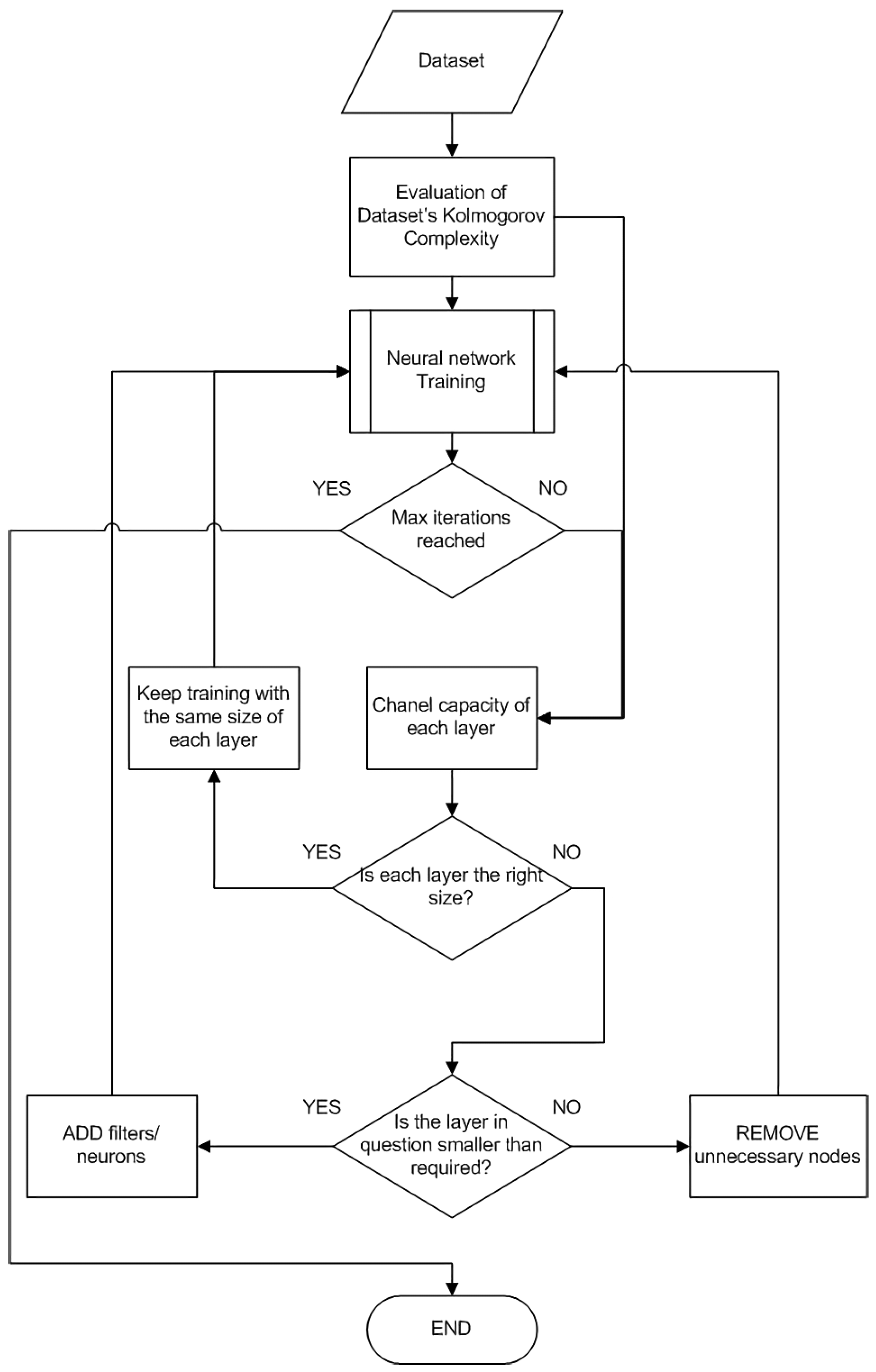
2. Outline of the Proposed Algorithm
- 1.
- At first, the complexity of the dataset is evaluated, using the average entropy, multiplied by the bits needed to depict each class (i.e., 3 bits for 8 classes).
- 2.
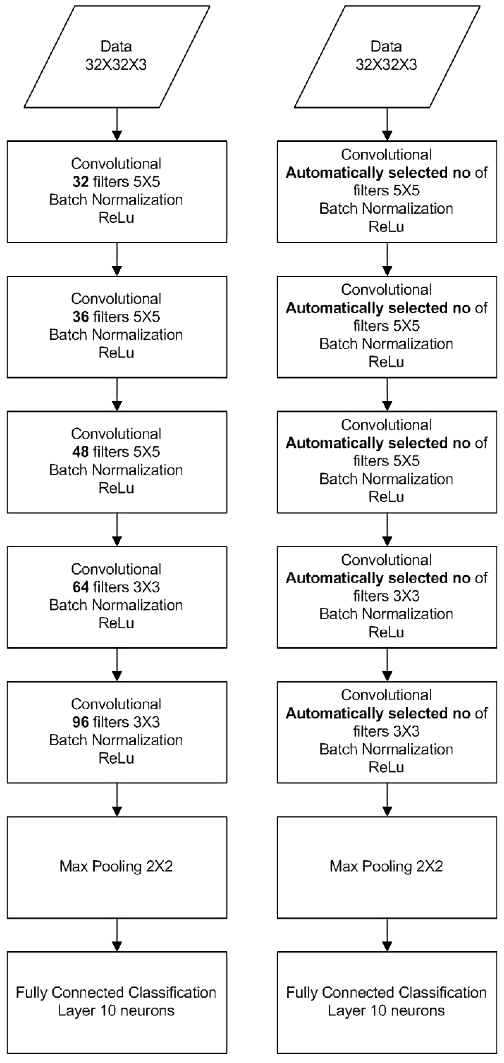
- The initial network topology is a common topology, i.e., a network topology used in the literature for similar datasets. The network is trained for a fixed number of epochs (e.g., 10), drifting from the random initialisation stage, in order to start encoding useful information in its layers.
- 3.
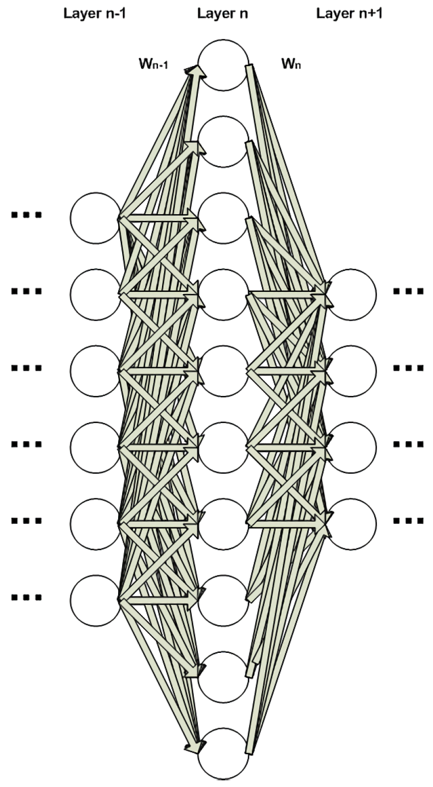
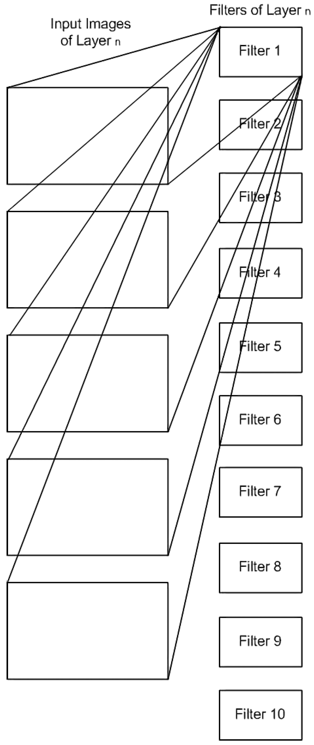
- After a number of epochs, the capacity of each layer is evaluated. Each layer is considered an information channel and the weight matrix can be viewed as a channel transition matrix (see (5)). We can then use a modified and optimized Blahut–Arimoto algorithm to estimate the information capacity of each layer. Based on the capacity of each layer and the given dataset complexity, extra filters are added with minimal weights (median 0, max 0.04 and min −0.04), so as not to undermine the training attained so far. In the case that the layer is found unable to contain the required information, we increase the width of those layers that are found to be too coarse, by adding new nodes with minimal weights. If a layer is found too wide, the nodes with the lowest entropy in their connections are removed. If the information capacity is found to lay within certain limits, no further action is taken. If there is no change of width of any layer for two consecutive iterations, the size of that layer freezes, and no computation takes place again for this specific part of the network.
- 4.
- The method terminates after a predefined number of epochs passes, or in the case that every layer size does not update.
3. Dataset Complexity Estimation
| Algorithm 1 Dataset complexity estimation |
|
4. Neural Network as an Information Channel—Capacity Estimation
4.1. The Blahut–Arimoto Algorithm
- 1.
- Start with an arbitrary
- 2.
- , where is the Kullback–Leibler divergence between the distributions of and .
- 3.
- Iterate 2, until convergence.
| Algorithm 2 The modified Blahut–Arimoto algorithm |
|
4.2. The Mutual Information Algorithm
| Algorithm 3 The mutual information algorithm |
|
5. Automated Neural Network Topology Optimization
5.1. Proposed Method Description
5.2. Method Application and Validation on the MNIST Dataset
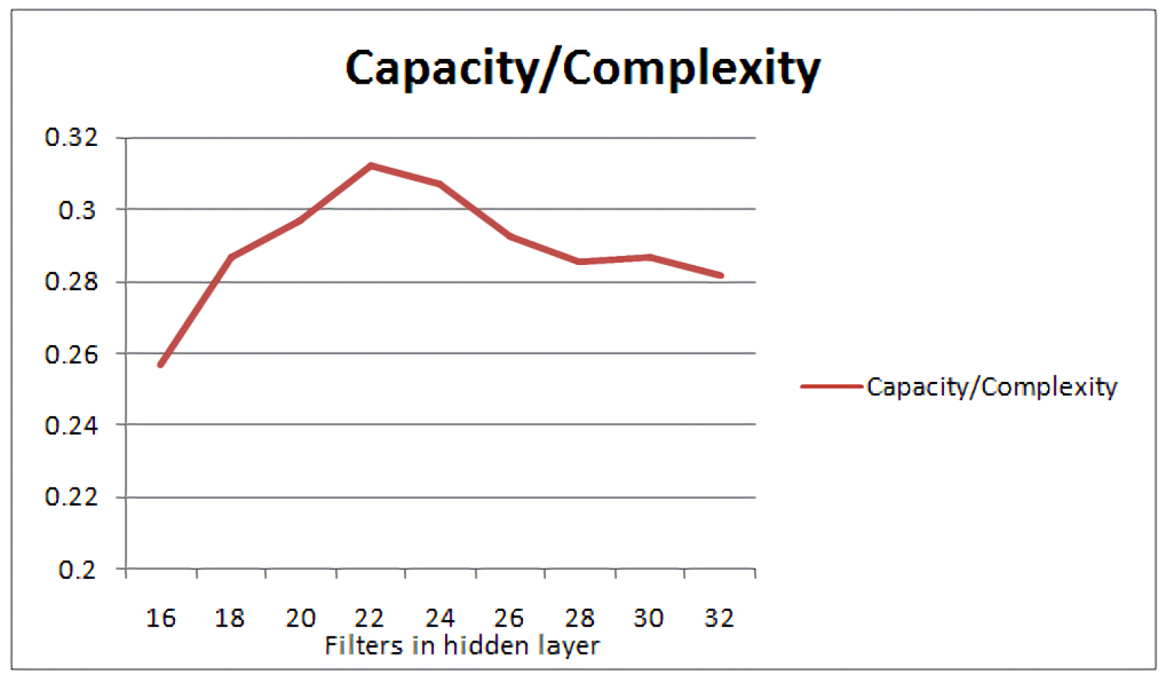
5.2.1. Optimal Layer Size Estimation
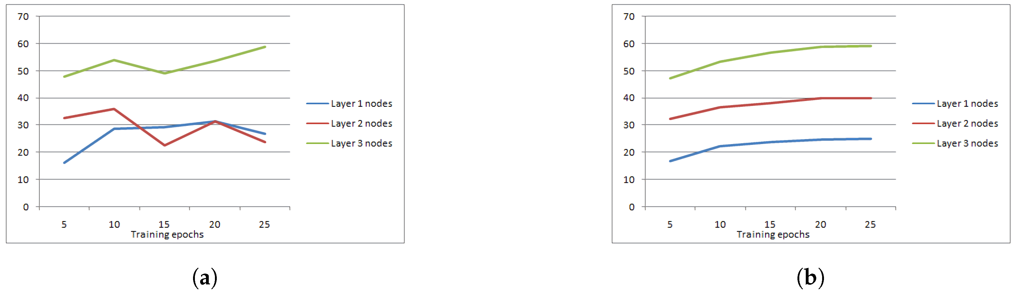
5.2.2. Information Capacity Evolution over More Layers and Network Adjustment
- Determine the complexity of the dataset;
- Set the desired capacity of the last layer equal to the dataset complexity;
- Set the desired capacity of each layer, according to (9);
- Begin training and, after a number of epochs, examine each layer independently;
- if the information capacity of the layer is larger than 1.05 of the desired capacity of the layer, remove nodes, according to (10);
- if the information capacity of the layer is smaller than 0.95 of the desired capacity of the layer, add nodes, according to (10);
- in all other cases, the layer stays the same;
- Go to 4 and continue the procedure, until the network is not updating or the accuracy is not improving.
5.2.3. Comparison between Blahut–Arimoto and Mutual Information for Layer Capacity Estimation
6. Experimental Results
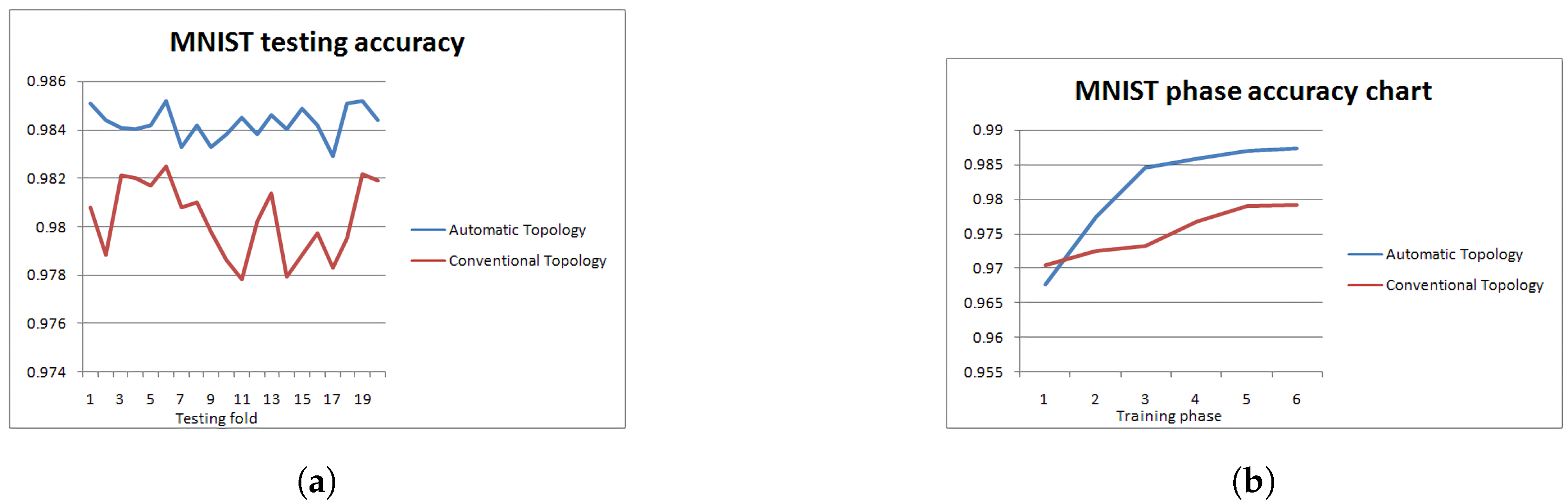
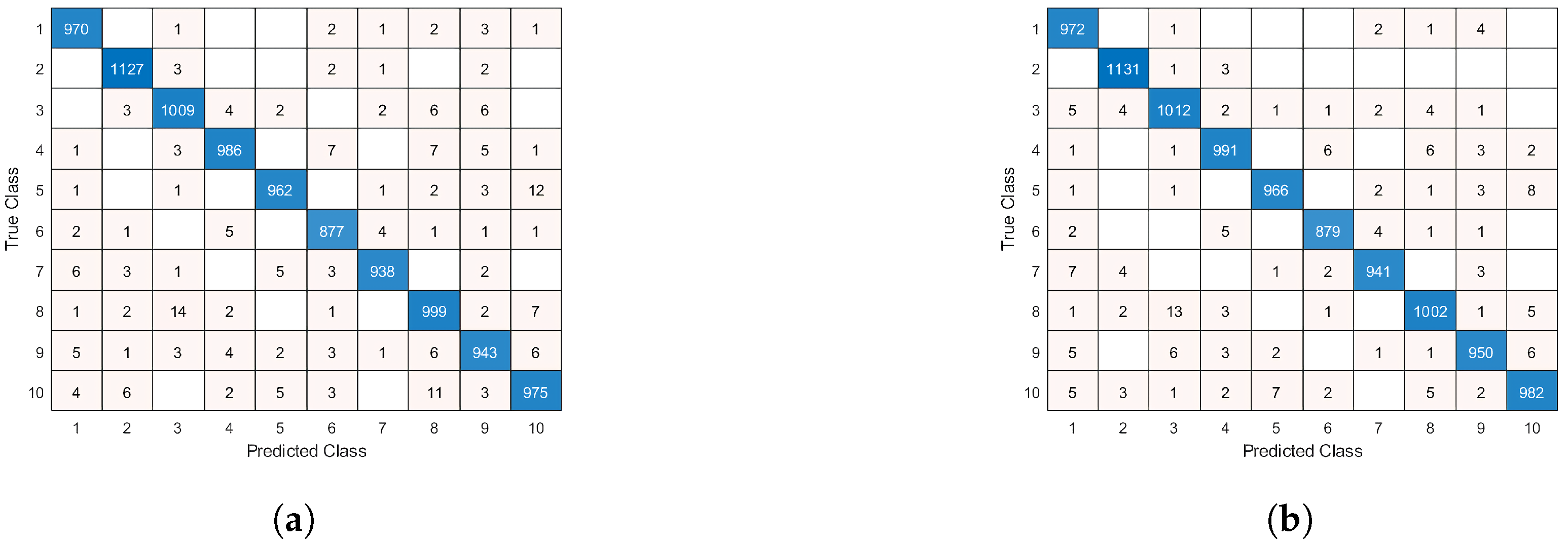
6.1. MNIST
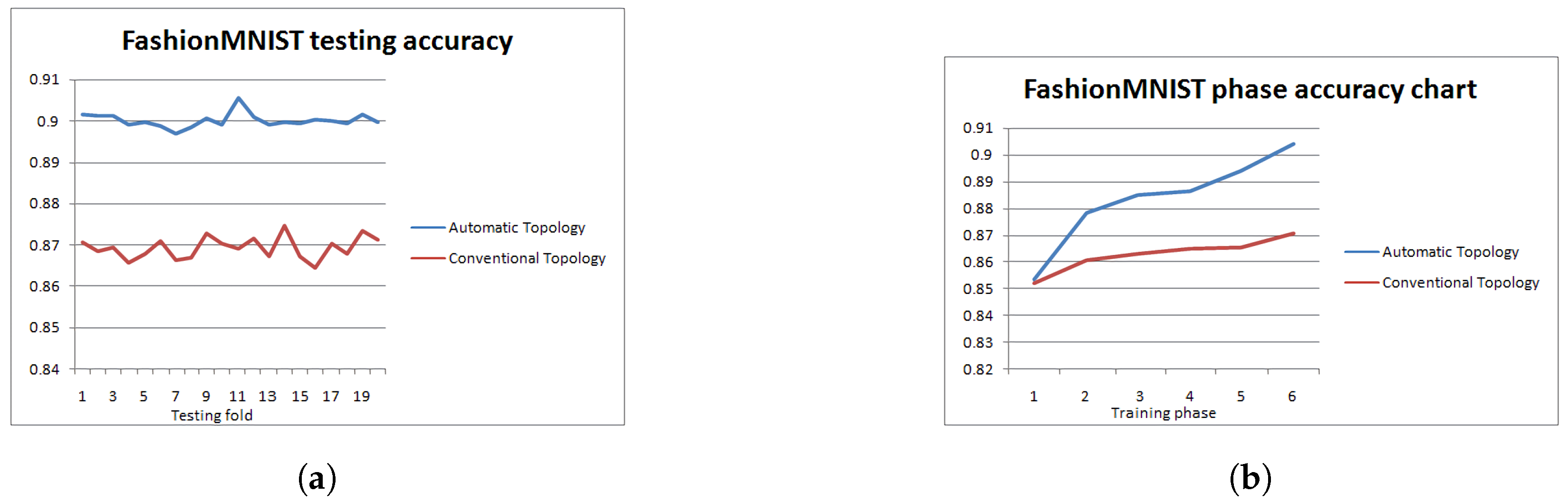
6.2. Fashion MNIST
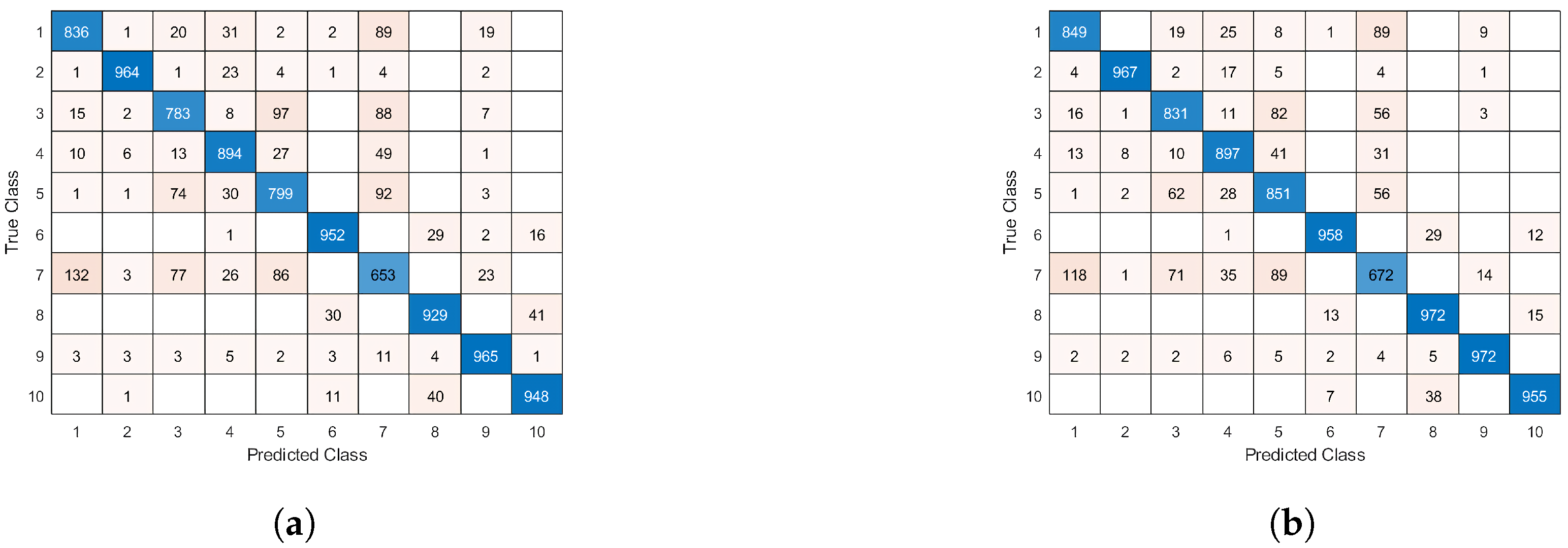
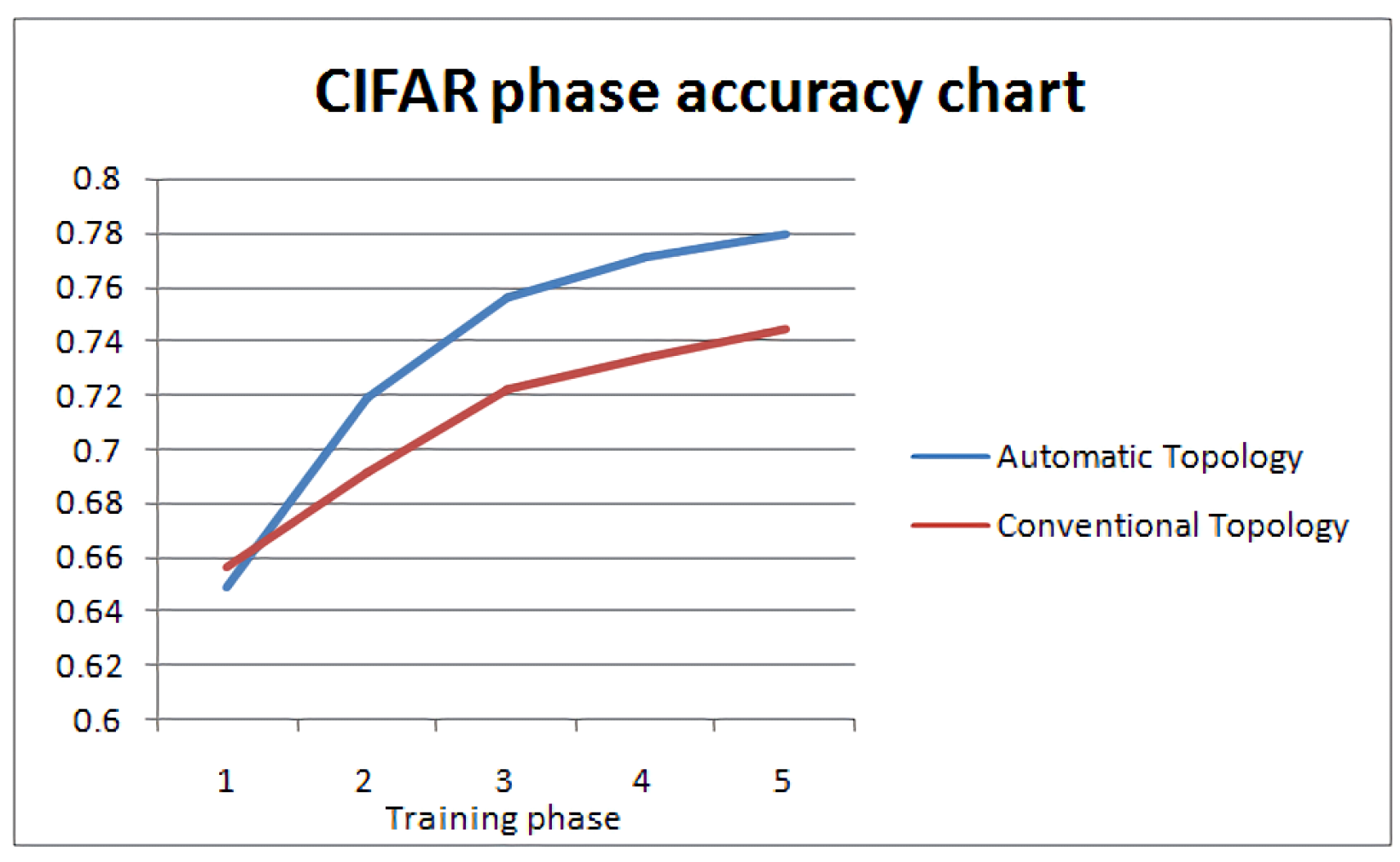
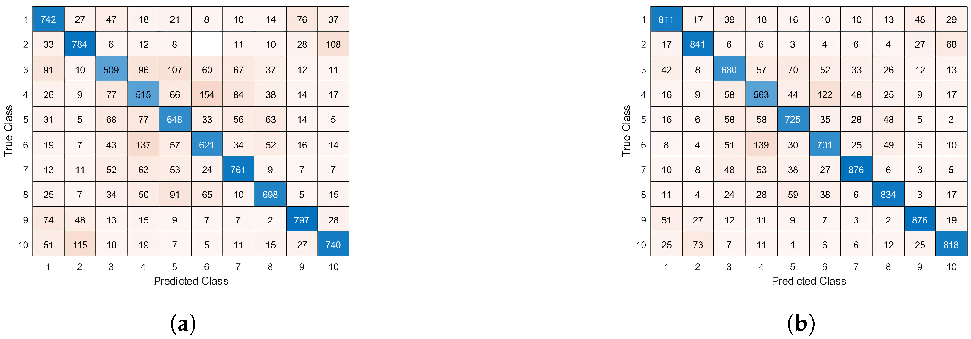
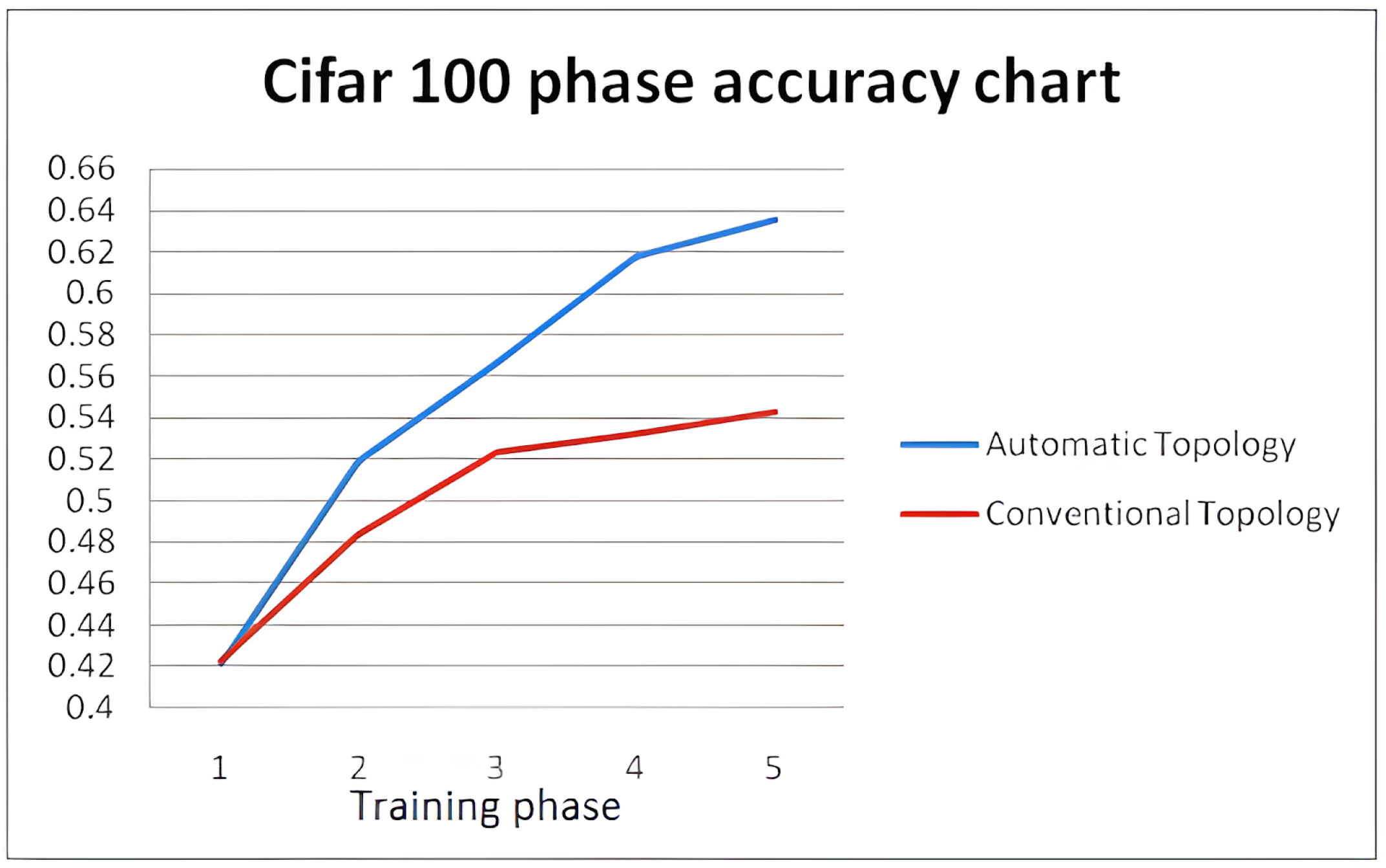
6.3. CIFAR-10 and CIFAR-100 Dataset
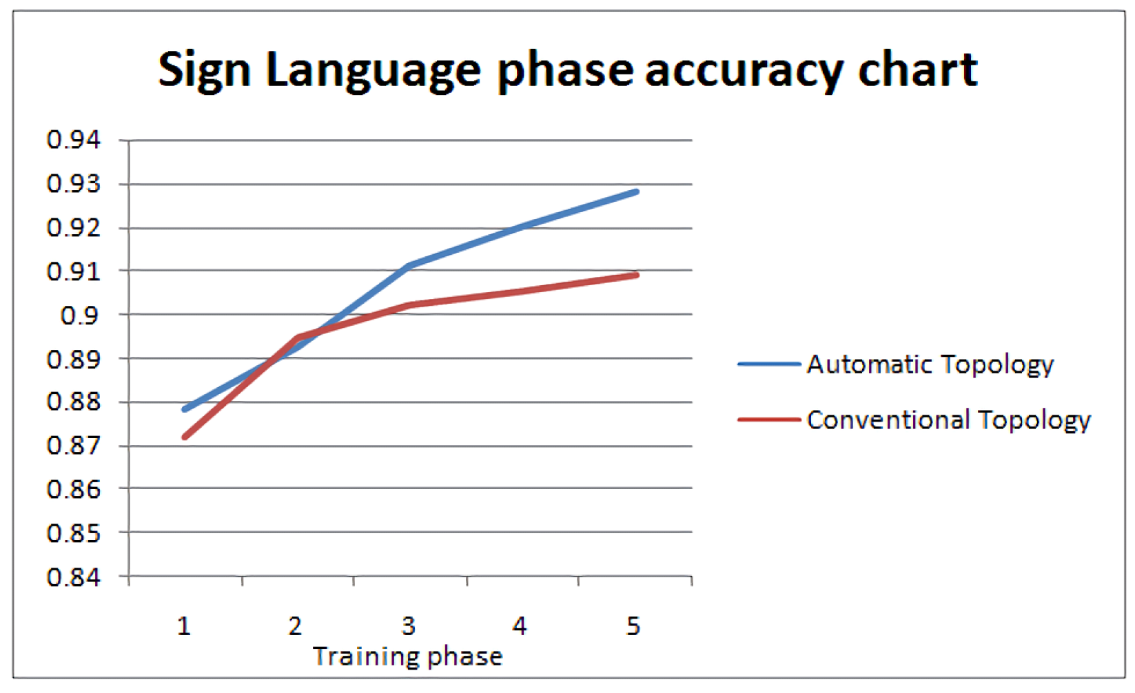
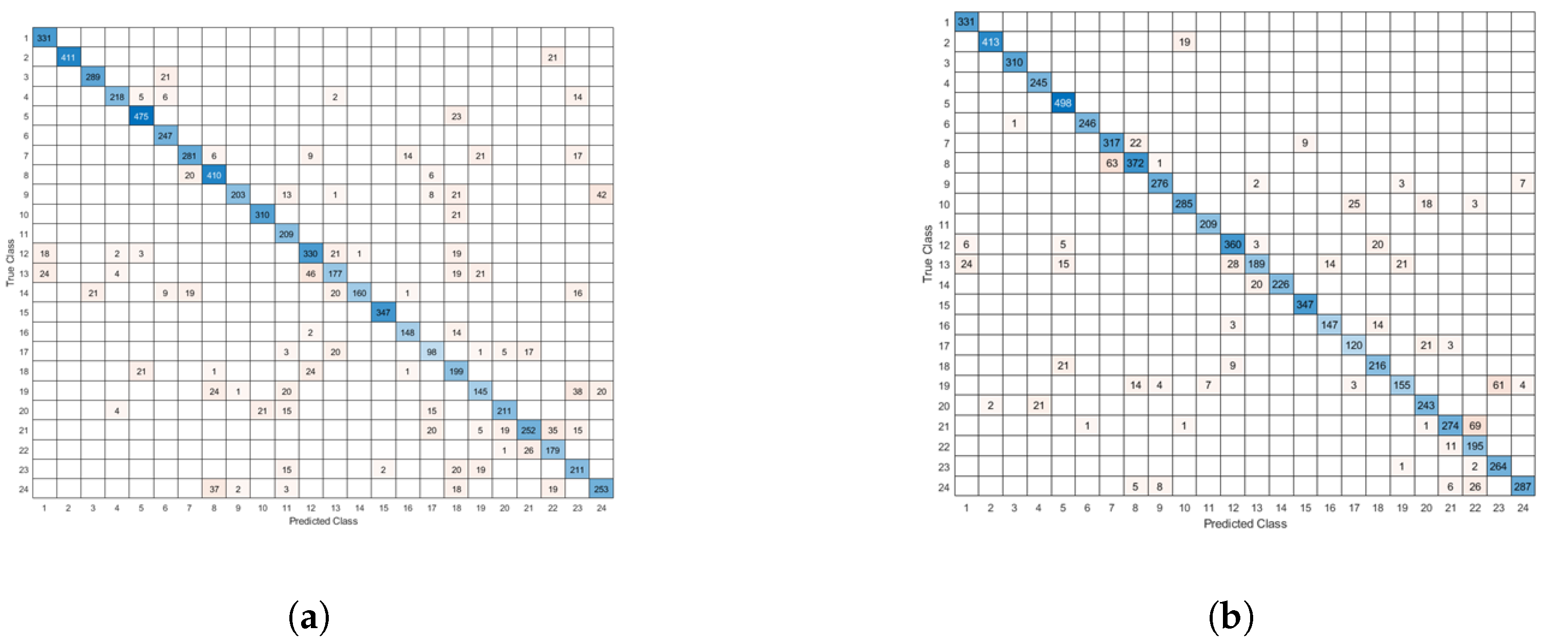
6.4. Sign Language Dataset
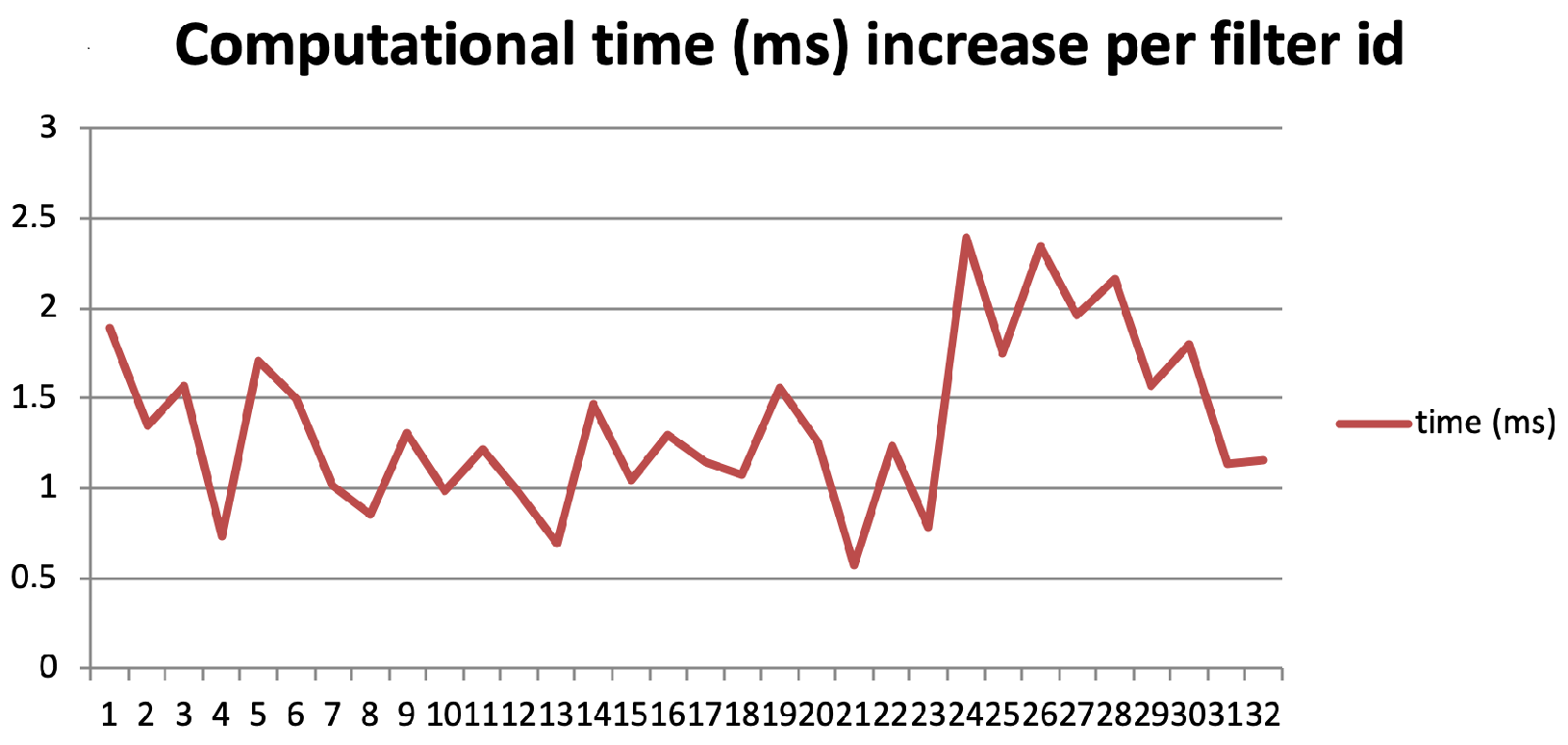
6.5. Computational Cost of the Proposed Algorithm
7. Conclusions—Future Work
Author Contributions
Funding
Institutional Review Board Statement
Informed Consent Statement
Data Availability Statement
Conflicts of Interest
References
- Siu, K.; Stuart, D.M.; Mahmoud, M.; Moshovos, A. Memory Requirements for Convolutional Neural Network Hardware Accelerators. In Proceedings of the 2018 IEEE International Symposium on Workload Characterization (IISWC), Raleigh, NC, USA, 30 September–2 October 2018; pp. 111–121. [Google Scholar] [CrossRef]
- Chen, T.; Li, M.; Li, Y.; Lin, M.; Wang, N.; Wang, M.; Xiao, T.; Xu, B.; Zhang, C.; Zhang, Z. MXNet: A Flexible and Efficient Machine Learning Library for Heterogeneous Distributed Systems. In Proceedings of the Neural Information Processing Systems, Workshop on Machine Learning Systems, Montreal, QC, Canada, 7–12 December 2015). [Google Scholar]
- Gruslys, A.; Munos, R.; Danihelka, I.; Lanctot, M.; Graves, A. Memory-Efficient Backpropagation Through Time. In Proceedings of the NIPS’16: 30th International Conference on Neural Information Processing Systems, Barcelona Spain, 5–10 December 2016. [Google Scholar]
- Diamos, G.; Sengupta, S.; Catanzaro, B.; Chrzanowski, M.; Coates, A.; Elsen, E.; Engel, J.; Hannun, A.; Satheesh, S. Persistent RNNs: Stashing recurrent weights on-chip. In Proceedings of the ICML’16: 33rd International Conference on International Conference on Machine Learning, New York, NY, USA, 19–24 June 2016; Volume 48, pp. 2024–2033. [Google Scholar]
- Hagan, M.; Demuth, H.B.; Beale, M.H.; De Jesus, O. Neural Network Design, 2nd ed.; Martin Hagan: Oklahoma, OK, USA, 2014; Available online: https://hagan.okstate.edu/nnd.html (accessed on 24 July 2022).
- Bishop, C. Neural Networks for Pattern Recognition; Oxford University Press: New York, NY, USA, 1995. [Google Scholar]
- Theodoridis, S. Machine Learning: A Bayesian Perspective, 1st ed.; Academic Press: Cambridge, MA, USA, 2015. [Google Scholar]
- Heaton, J. Introduction to Neural Networks for Java, 2nd ed.; Heaton Research, Inc.: Dublin, Ireland, 2008. [Google Scholar]
- Han, S.; Mao, H.; Dally, W.J. Deep compression: Compressing deep neural network with pruning, trained quantization and huffman coding. In Proceedings of the 4th International Conference on Learning Representations, ICLR 2016, San Juan, Puerto Rico, 2–4 May 2016; Available online: http://arxiv.org/abs/1510.00149 (accessed on 24 July 2022).
- Lee, N.; Ajanthan, T.; Torr, P.H.S. Snip: Single-shot network pruning based on connection sensitivity. In Proceedings of the 7th International Conference on Learning Representations, ICLR 2019, New Orleans, LA, USA, 6–9 May 2019; Available online: https://openreview.net/forum?id=B1VZqjAcYX (accessed on 24 July 2022).
- Li, H.; Kadav, A.; Durdanovic, I.; Samet, H.; Graf, H.P. Pruning filters for efficient convnets. arXiv 2016, arXiv:1608.08710. [Google Scholar]
- Frankle, J.; Carbin, M. The lottery ticket hypothesis: Finding sparse, trainable neural networks. In Proceedings of the 7th International Conference on Learning Representations, ICLR 2019, New Orleans, LA, USA, 6–9 May 2019; Available online: https://openreview.net/forum?id=rJl-b3RcF7 (accessed on 24 July 2022).
- Liu, Z.; Sun, M.; Zhou, T.; Huang, G.; Darrell, T. Re-thinking the value of network pruning. In Proceedings of the 7th International Conference on Learning Representations, ICLR 2019, New Orleans, LA, USA, 6–9 May 2019; Available online: https://openreview.net/forum?id=rJlnB3C5Ym (accessed on 24 July 2022).
- Han, S.; Pool, J.; Tran, J.; Dally, W. Learning both weights and connections for efficient neural network. In Proceedings of the NIPS’15: Proceedings of the 28th International Conference on Neural Information Processing Systems, Montreal, QC, Canada, 7–12 December 2015; pp. 1135–1143. [Google Scholar]
- Gale, T.; Elsen, E.; Hooker, S. The state of sparsity in deep neural networks. arXiv 2016, arXiv:1902.09574. [Google Scholar]
- Frankle, J.; Dziugaite, G.K.; Roy, D.M.; Carbin, M. The lottery ticket hypothesis at scale. arXiv 2019, arXiv:1903.01611. [Google Scholar]
- Cover, T.M.; Thomas, J.A. Elements of Information Theory, 2nd ed.; Wiley-Interscience: Hoboken, NJ, USA, 2006; pp. 206–207. ISBN 978-0-471-24195-9. [Google Scholar]
- Kolmogorov, A. On Tables of Random Number. Theor. Comput. Sci. 1998, 207, 387–395. [Google Scholar] [CrossRef]
- Kolmogorov, A.N. Three Approaches to the Quantitative Definition of Information. Probl. Inform. Transm. 1965, 1, 1–7. [Google Scholar] [CrossRef]
- Kolmogorov, A.X. Logical basis for information theory and probability theory. IEEE Trans. Inf. Theory 1968, 14, 662–664. [Google Scholar] [CrossRef]
- Arimoto, S. An algorithm for computing the capacity of arbitrary discrete memoryless channels. IEEE Trans. Inf. Theory 1972, 18, 14–20. [Google Scholar] [CrossRef]
- Burgin, M. Generalized Kolmogorov complexity and duality in theory of computations. Not. Russ. Acad. Sci. 1982, 25, 19–23. [Google Scholar]
- Vitányi, P.M.B. Conditional Kolmogorov complexity and universal probability. Theor. Comput. Sci. 2013, 501, 93–100. [Google Scholar] [CrossRef]
- Kaltchenko, A. Algorithms for Estimating Information Distance with Application to Bioinformatics and Linguistics. arXiv 2004, arXiv:cs.CC/0404039. [Google Scholar]
- Solomonoff, R. A Preliminary Report on a General Theory of Inductive Inference; Report V-131; Revision Published November 1960; Zator Company: Cambridge, MA, USA, 1960. [Google Scholar]
- Rissanen, J. Information and Complexity in Statistical Modeling; Springer: Berlin/Heidelberg, Germany, 2007; p. 53. ISBN 978-0-387-68812-1. [Google Scholar]
- Blahut, R. Computation of channel capacity and rate-distortion functions. IEEE Trans. Inf. Theory 1972, 18, 460–473. [Google Scholar] [CrossRef]
- Vontobel, P.O. A Generalized Blahut–Arimoto Algorithm. In Proceedings of the IEEE International Symposium on Information Theory, Yokohama, Japan, 29 June–4 July 2003. [Google Scholar]
- Naiss, I.; Permuter, H.H. Extension of the Blahut–Arimoto Algorithm for Maximizing Directed Information. IEEE Trans. Inf. Theory 2013, 59, 204–222. [Google Scholar] [CrossRef]
- Jetka, T.; Nienaltowski, K.; Winarski, T.; Blonski, S.; Komorowski, M. Information-theoretic analysis of multivariate single-cell signaling responses. PLoS Comput. Biol. 2019, 15, e1007132. [Google Scholar] [CrossRef] [PubMed]
- Yu, Y. Squeezing the Arimoto-Blahut Algorithm for Faster Convergence. IEEE Trans. Inf. Theory 2010, 56, 3149–3157. [Google Scholar] [CrossRef]
- Krizhevsky, A. Learning Multiple Layers of Features from Tiny Images. 2009. Available online: https://www.cs.toronto.edu/~kriz/learning-features-2009-TR.pdf (accessed on 24 July 2022).
- Siddiqui, S.A.; Salman, A.; Malik, I.; Shafait, F. Automatic fish species classification in underwater videos: Exploiting pretrained deep neural network models to compensate for limited labelled data. ICES J. Mar. Sci. 2018, 75, 374–389. [Google Scholar] [CrossRef]
- Shannon, C.E. A Mathematical Theory of Communication. Bell Syst. Tech. J. 1948, 27, 379–423. [Google Scholar] [CrossRef]
- Deng, L. The mnist database of handwritten digit images for machine learning research. IEEE Signal Proc. 2012, 29, 141–142. [Google Scholar] [CrossRef]
- Support Vector Machines Speed Pattern Recognition—Vision Systems Design. 2004. Available online: https://www.vision-systems.com/home/article/16737424/support-vector-machines-speed-pattern-recognition (accessed on 24 July 2022).
- LeCun, Y.; Cortez, C.; Burges, C.C.J. The MNIST Handwritten Digit Database. Yann LeCun’s Website. 2020. Available online: http://yann.lecun.com (accessed on 24 July 2022).
- Kussul, E.; Baidyk, T. Improved method of handwritten digit recognition tested on MNIST database. Image Vis. Comput. 2004, 22, 971–981. [Google Scholar] [CrossRef]
- Belilovsky, E.; Eickenberg, M.; Oyallon, E. Greedy Layerwise Learning Can Scale to ImageNet. arXiv 2019, arXiv:abs/1812.11446. [Google Scholar]
- Maniatopoulos, A.; Gazis, A.; Pallikaras, V.P.; Mitianoudis, N. Artificial Neural Network Performance Boost using Probabilistic Recovery with Fast Cascade Training. Int. J. Circuits Syst. Signal Process. 2020, 14, 847–854. [Google Scholar] [CrossRef]


| Conv. Filters | Capacity | Accuracy | Capacity/(Layer’s Complexity) |
|---|---|---|---|
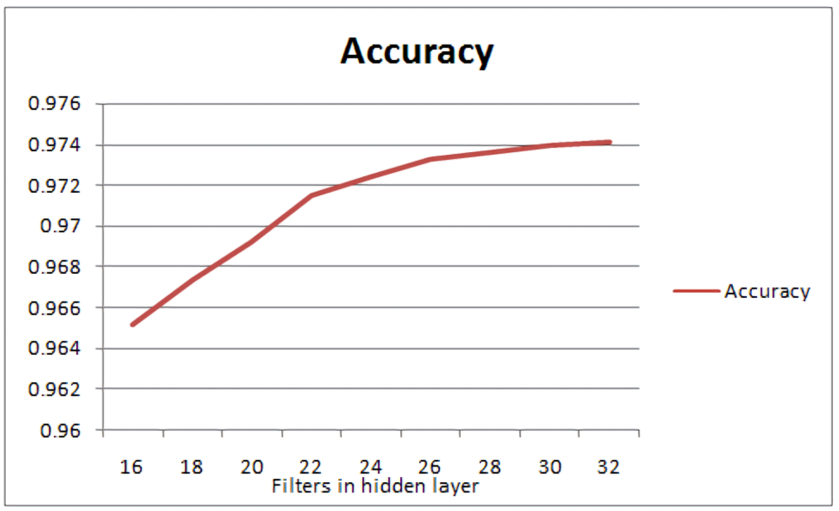
| 16 | 4.1061 | 0.9652 | 0.25663125 |
| 18 | 5.1617 | 0.9674 | 0.286761111 |
| 20 | 5.937 | 0.9692 | 0.29685 |
| 22 | 6.8649 | 0.9715 | 0.3120409091 |
| 24 | 7.371 | 0.9724 | 0.307125 |
| 26 | 7.608 | 0.9733 | 0.292615384 |
| 28 | 7.9864 | 0.9736 | 0.285228571 |
| 30 | 8.599 | 0.9739 | 0.28663333 |
| 32 | 9.008 | 0.9741 | 0.2815 |
| Conv. Filters | Accuracy | First Order Derivative (Using MVT) |
|---|---|---|
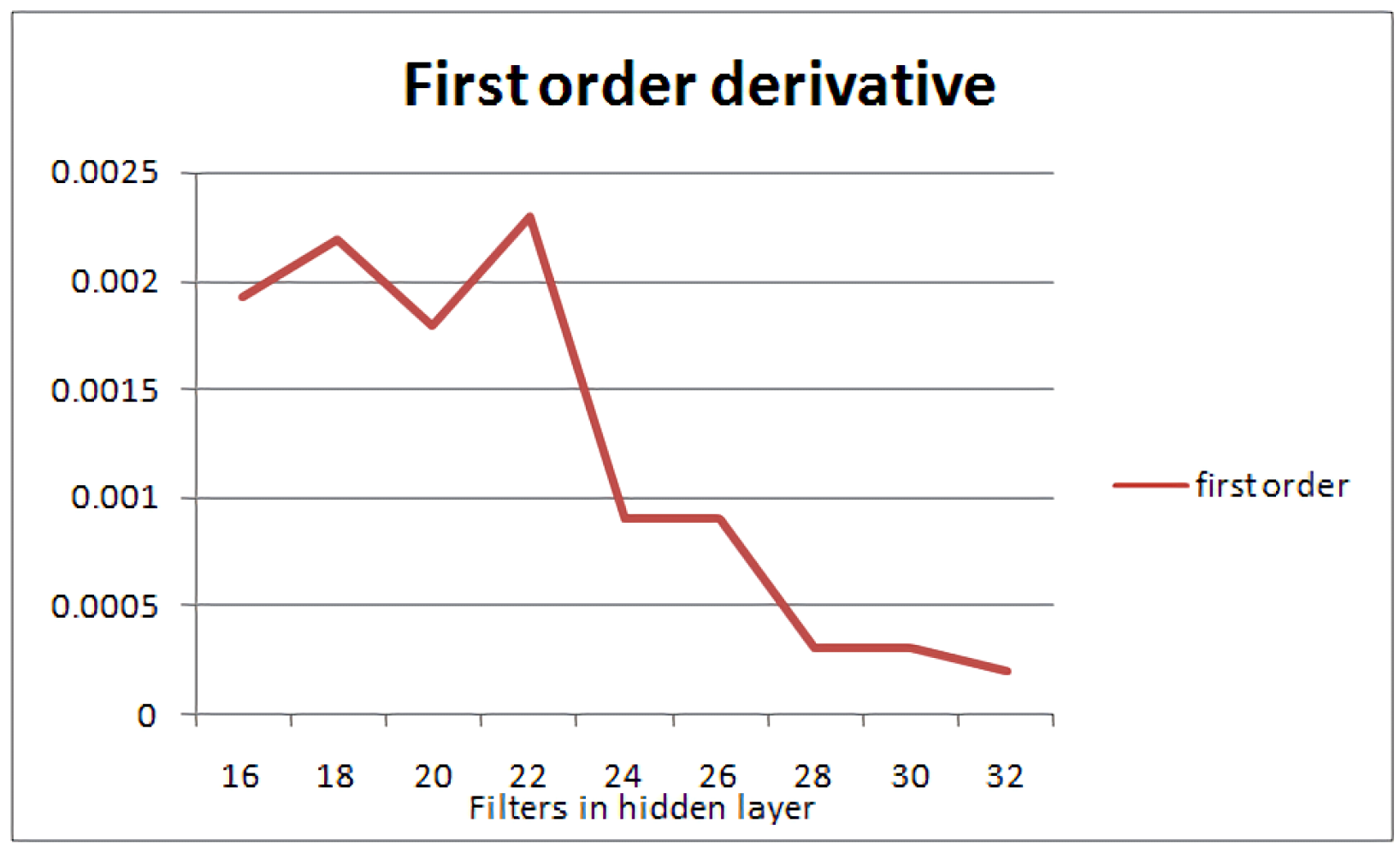
| 16 | 0.9652 | 0.0019 |
| 18 | 0.9674 | 0.0022 |
| 20 | 0.9692 | 0.0018 |
| 22 | 0.9715 | 0.0023 |
| 24 | 0.9724 | 0.0009 |
| 26 | 0.9733 | 0.0009 |
| 28 | 0.9736 | 0.0003 |
| 30 | 0.9739 | 0.0003 |
| 32 | 0.9741 | 0.0002 |
Publisher’s Note: MDPI stays neutral with regard to jurisdictional claims in published maps and institutional affiliations. |
© 2022 by the authors. Licensee MDPI, Basel, Switzerland. This article is an open access article distributed under the terms and conditions of the Creative Commons Attribution (CC BY) license (https://creativecommons.org/licenses/by/4.0/).
Share and Cite
Maniatopoulos, A.; Alvanaki, P.; Mitianoudis, N. OptiNET—Automatic Network Topology Optimization. Information 2022, 13, 405. https://doi.org/10.3390/info13090405
Maniatopoulos A, Alvanaki P, Mitianoudis N. OptiNET—Automatic Network Topology Optimization. Information. 2022; 13(9):405. https://doi.org/10.3390/info13090405
Chicago/Turabian StyleManiatopoulos, Andreas, Paraskevi Alvanaki, and Nikolaos Mitianoudis. 2022. "OptiNET—Automatic Network Topology Optimization" Information 13, no. 9: 405. https://doi.org/10.3390/info13090405
APA StyleManiatopoulos, A., Alvanaki, P., & Mitianoudis, N. (2022). OptiNET—Automatic Network Topology Optimization. Information, 13(9), 405. https://doi.org/10.3390/info13090405