Abstract
Physiological and kinematic signals from humans are often used for monitoring health. Several processes of interest (e.g., cardiac and respiratory processes, and locomotion) demonstrate periodicity. Training models for inference on these signals (e.g., detection of anomalies, and extraction of biomarkers) require large amounts of data to capture their variability, which are not readily available. This hinders the performance of complex inference models. In this work, we introduce a methodology for improving inference on such signals by incorporating phase-based interpretability and other inference tasks into a multi-task framework applied to a generative model. For this purpose, we utilize phase information as a regularization term and as an input to the model and introduce an interpretable unit in a neural network, which imposes an interpretable structure on the model. This imposition helps us in the smooth generation of periodic signals that can aid in data augmentation tasks. We demonstrate the impact of our framework on improving the overall inference performance on ECG signals and inertial signals from gait locomotion.
1. Introduction
In recent years, time series have gained attention in the scientific community due to their importance in numerous applications (e.g., computer vision, and natural language processing). There are many studies in the literature trying to model these signals with different techniques to improve state-of-the-art performance for different tasks [1,2,3,4]. Modeling times series, in general, is a particularly challenging task due to many factors, such as uncertainty, quality of data acquisition, and data scarcity, to name a few [3,4,5]. These factors worsen when signals are collected from physiological processes and wearable devices due to the quality of the devices and human factors. These factors make modeling the data extremely difficult. On top of the aforementioned reasons, another important issue with modeling these types of time series are the complex underlying dynamics, which can change drastically over time. These dynamics are the key to successfully understanding how those signals behave. There are some studies that have tried to tackle some of these issues for different tasks (e.g., classification, and forecasting) by leveraging deep neural networks to model the signals [6,7,8,9]. Some authors use recurrent neural networks (RNNs) and convolutional neural networks (CNNs) for long-term and short-term prediction [6,7,8,9]. Prior work has also used attention mechanisms and transformers [10,11] to extract relevant information for forecasting. Others use ordinary differential equations (ODEs) solvers [12,13] to model the signals directly. Some of these frameworks can be interpreted as a continuous version of ResNet [12]. In this paper, we focus on forecasting and classification while addressing the challenges applied to physiological and inertial data.
Deep neural networks typically have thousands if not millions of parameters, which makes it difficult to understand how information flows from input to output. Despite having high accuracy and good performance, it was shown in [14] that sometimes, the models do not necessarily pick relevant information to reach a high level of accuracy. Being able to provide an interpretation of how the model picks the features can make them more reliable for specific applications (e.g., medical). There has been effort in computer vision and natural language processing to provide some interpretability on how the models perform prediction [15,16]. Specifically, most of these methods are limited to explaining the classification task. One way to provide explainability is to add an interpretable unit (very simple neural network) to the model in the training process [16,17,18]. Authors in [17,18] worked on interpretability for times series to be able to explain the process with which their models make decisions. The interpretability in this paper follows the methodology in [16] where a separate unit is used to impose structure on the model. In our case, since the signals are periodic, we use phase information as a means to impose structure. In Section 3.4 and Section 3.6, we provide more explanation on the details of the process and how this interpretability can help us with signal generation.
For medical applications, a reliable, robust, and interpretable model is crucial for decision making. In this work, we focus on measurements from wearable devices and sensors that collect inertial measurement unit (IMU) data, consisting of gyroscope, accelerometer, and also electrocardiography (ECG) signals. In [19], the authors use IMU signals in conjunction with some video information to perform forecasting and classification for terrain change for wearable robotic applications. Forecasting, in this case, will help patients to experience a smooth impedance transition from one terrain to another. In the case of ECG signals, reliable forecasting would play a significant role in patients’ health. We use these signals to perform prediction, forecasting, classification, and signal generation. Generating realistic signals in this application can be especially useful due to the difficulty of data collection and scarcity.
The main motivation for this paper is leveraging multi-task learning, including inference tasks (classification and forecasting) and phase-based interpretability to improve model performance and explainability. It was shown in [3,4,20,21] that model performance can be improved by using multi-task learning. In the following, we summarize our contributions:
- Infusing phase information to the input and as a regularizer to improve model performance.
- Adding a unit for inducing interpretability for periodic physiological and sensory data.
- Exploring the trade-off between performance and interpretability for better understanding the underlying system.
- Generating synthetic sensory data by leveraging the interpretable unit.
As far as the authors are aware, there is no other work which combines multi-task learning with interpretability based on phase information and explores the trade-off between model performance and explainability on physiological periodic signals.
The organization of the paper is as follows. In Section 2, we introduce the notations, formulate the problem, and thoroughly explore different parts of the problem. In Section 3, we conduct experiments to verify our claims in this paper. We discuss the results in Section 4 and conclude the paper in Section 5.
2. Materials and Methods
2.1. Mathematical Formulation
A time-dependent signal , where indicates the number of channels in the signal, is considered. The signal is processed over a window of length . The signal over a fixed window , with t indicating the current time, is denoted by . The signal is accompanied by a derived phase angle , which is available over the same window. In general, an auto-encoder structure can be imposed in this problem, such that
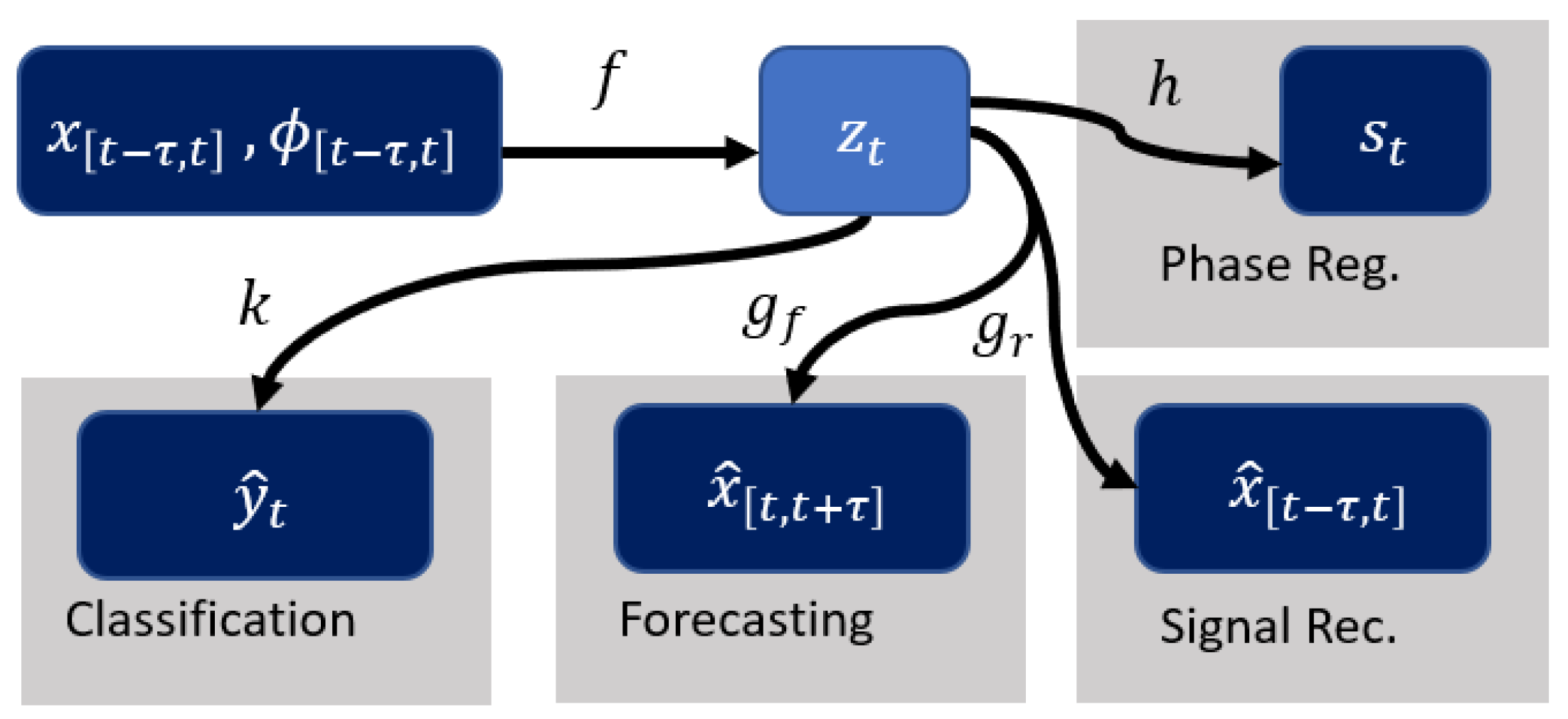
where f is the encoder and g is the decoder. As shown in Figure 1, more structure is introduced by using as an additional input and encoding the phase information using the function (see Section 2.2). This structure allows to incorporate phase to the model for multi-task learning and interpretability. This gives a new set of equations:
where f is the encoder and is the decoder for the signal, and h is used to recover a summary of the phase (denoted as ) employed for regularization (see Section 2.2).
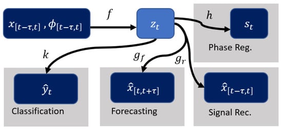
Figure 1.
Illustration of multi-task and interpretability pipeline. f represents the encoder and maps the input to . The decoder is split into for reconstructing the input signal and for forecasting. k is the network for classification. h takes care of estimation of the phase summary for regularization purposes.
The main inference tasks under consideration are signal forecasting and classification. Additional functions of the latent representation are introduced to accommodate these predictions, which are given in the following form
where and k are the forecasting and classification networks. It is noted that we have specified the forecasting to be over a window of size for simplicity and this can be generalized without any restrictions.
We focus on signal reconstruction and forecasting in our use cases when quantifying performance. The model will be trained by considering different combinations of the inference and regularization tasks. The overall loss function for training has the form
where the first two terms correspond to the reconstruction of and a regularization term on to improve interpretability, and the last two terms correspond to forecasting and classification tasks, respectively.
Details about the different components of this model are described in the remainder of this section. Each term in the loss function is introduced in detail.
2.2. Phase Computation and Encoding
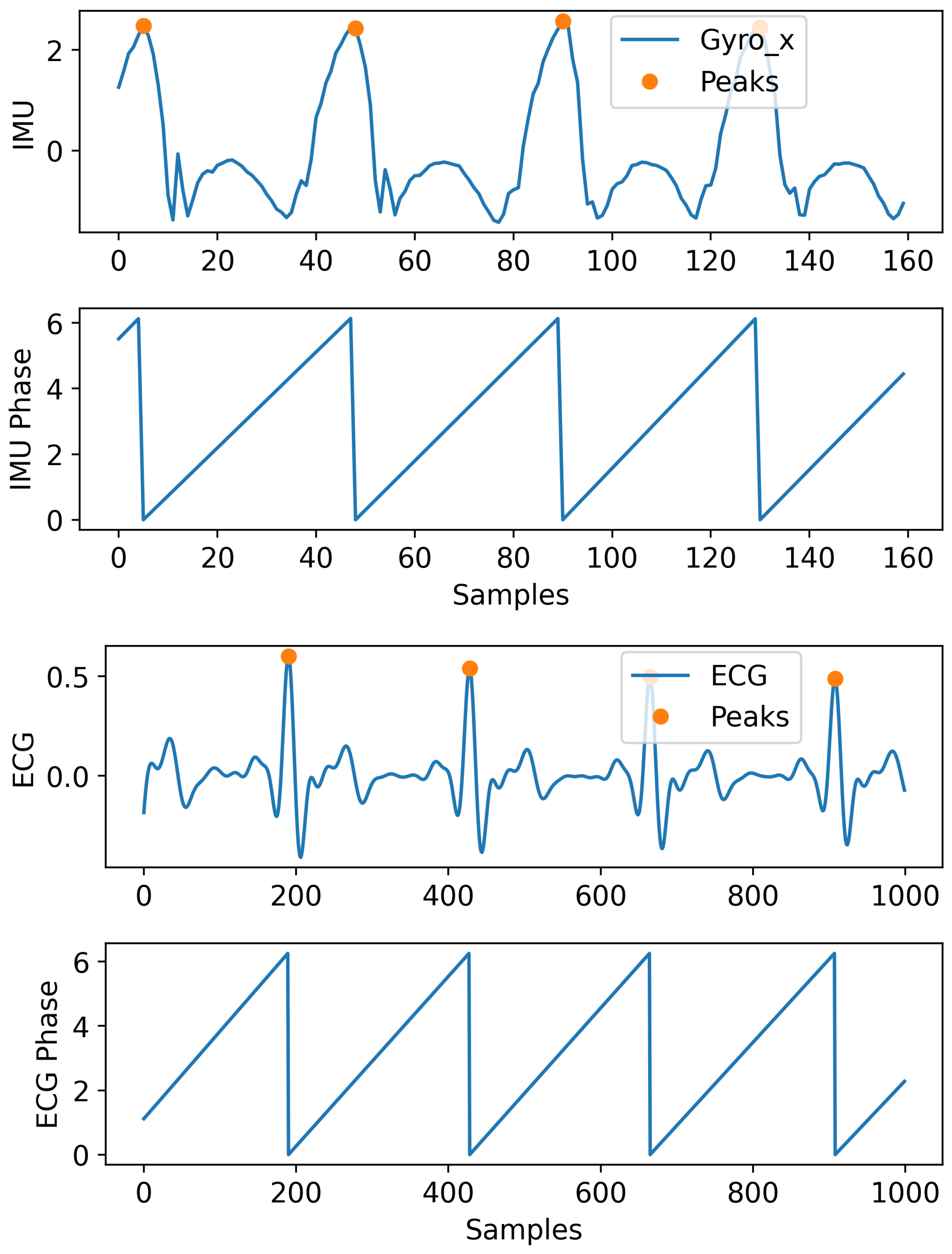
In periodic signals, the phase information can be very helpful in modeling the signals’ dynamic. In this section, we explain the procedure used to incorporate the phase in the signal modeling. In Figure 2, we show an example of the IMU and ECG signals used for our applications and how their phase information was extracted. We calculated the phase by using peak detection to account for any variability in the frequency. Peaks are located and used to perform temporal alignment between consecutive periods by normalizing the time window to the interval . A phase is assigned to each period of the signal based on its phase on the standard interval. It is shown that this information can help the model to improve the performance compared to when this information is not incorporated.
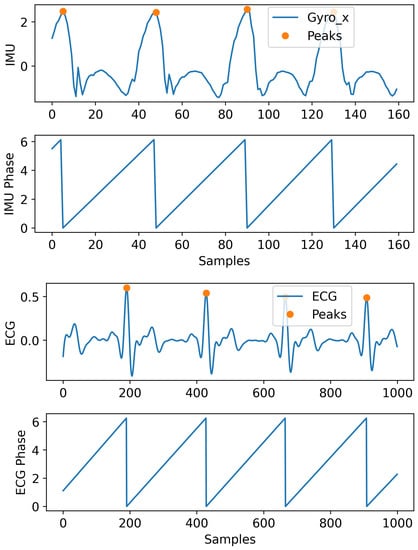
Figure 2.
Showing IMU (only a single channel for illustration) and ECG signal with their peaks and extracted phase (in radians) information.
We further encode the phase value for a window using the function which represents either a one-hot or Gaussian encoding. The latter builds on the one-hot encoding by centering a narrow Gaussian function around the non-zero component of the array. This allows for a more continuous encoding of the phase rather than a discrete one. Intuitively speaking, one may think that the one-hot version is less noisy (having just one non-zero component in each array) than the Gaussian version, which indicates that the one-hot version might have better performance; however, this is not what it is observed empirically. To summarize the above description: first, we calculate the phase for a given window, then we calculate the one-hot encoded (or Gaussian) version of the phase using the function. The raw phase is used as part of the latent space regularization, and the encoded version of historic values is concatenated to the input. In Section 3.3, we thoroughly explain and compare these two encoding schemes.
2.3. Signal Encoder and Decoder Architecture
We use an auto-encoder architecture for modeling the signals. This architecture will allow us to impose meaningful restrictions on the latent dimensions for interpretability purposes. The encoder, f, consists of a featured network that downsamples the input and passes it into an ODE-Net to map the data to a certain latent space. Details on the architecture can be seen in the Appendix A.2. Both networks are composed of linear and convolutional layers. The decoder g is another convolutional network that maps the encoder output back to the original input space. Network g is divided into two portions, as shown in Figure 1, where shows reconstruction for the original input to the model while shows the forecasted signal. The loss function for reconstruction becomes as follows:
where and are the input and the corresponding output of the model with and representing the number of training samples, length of the window and number of channels in a signal, respectively.
2.4. Phase Regularization
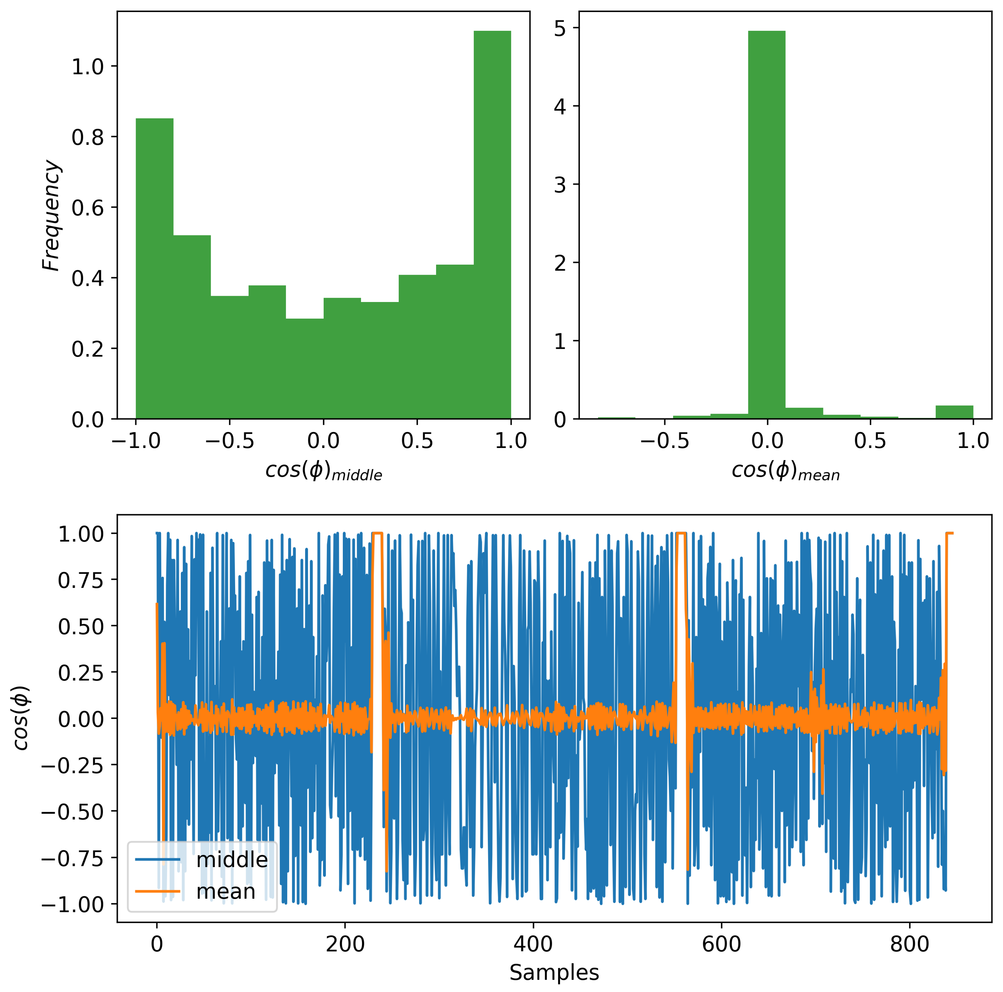
In order to use some information about the phase of the signal as a way of regularizing our model, we extract a summary from the phase . We use a summary to avoid having to reconstruct a full phase and reduce the number of parameters in our model. We consider two summaries: (1) the phase value in the middle of a window, and (2) the mean phase value of a window. For the discussion in this section, the phase values are initially represented using a unit-vector representation in corresponding to the cosine and sine of the corresponding phase angle. As described before, we use a window of data as the input to the model. In case of the middle phase, for each window, we choose the middle element as a representation of the phase to be reconstructed. In this way, we evade the problem that we have with the mean phase. We obtain a mean phase over a window by averaging the continuous phase vectors. Unfortunately, this process does not provide an informative summary of the phase over a window. This is because the mean phase tends to go to zero due to the nature of the oscillating signals, and our choice of which covers a few periods of the signals. In Figure 3 (bottom), we show what the cosine component of the phase vector looks like for both the mean and middle phases. As it can be observed, most of the mean phases are close to zero. We also provide the histograms in Figure 3 (top) for both cases to observe their spread. We observe empirically that the middle phase summary leads to the best performance. So, for all the experiments performed in this paper, we use the middle phase.

Figure 3.
Comparing the cosine component of two phase modalities. (Bottom) The mean phase shows less variability compared to the middle phase. (Top) The histogram of the mean phases (right) maps most values near zero while the middle phase (left) has a greater spread distribution.
Next, we discuss the choices for learning the phase summary through h as shown in Figure 1. We explore two possibilities for h:
The first choice relies directly on the latent space to capture phase information while the other introduces a new neural network, L, to map the latent space to a 2D space to induce interpretability and regularization. Remember that we use a unit-vector representation for the phase summary . In the second case, we have more flexibility in the data modeling due to the non-linear transformations applied by the network L.
For neural networks, it is often valuable to add structure to the network to give us some insight on what is being learned. To do so, we add two terms in the regularization loss . The first imposition corresponds to the phase reconstruction term. The second term ensures that the radius of our reconstructed phase stays around one. These two terms are defined as follows:
and
then
where and are the predicted and the ground-truth phase summaries, respectively. The hyper-parameters and are chosen empirically. We go into detail on how these parameters are chosen in Section 3.2. It is shown that there is a meaningful relationship between these two hyper-parameters that can help us pick them more carefully for interpretability. The first term helps make the latent space more structured and more interpretable for the cyclic behavior of the periodic signals. The second term imposes the magnitude restriction to avoid having outliers in the latent space, which may not necessarily correspond to the actual signal and to make the latent space a bit more compact. Intuitively, this compactness helps with data modeling. We discuss more on the effect of these terms in subsequent sections.
2.5. Forecasting Task
As it is shown in Figure 1, forecasting is one of the inference tasks considered. This is a challenging task in time series, which motivates our paper to improve its performance [2]. When forecasting is included, our reconstruction network is expanded to return . This means that the first portion of the output is associated with and the reconstructed signal , and the second half is associated with and the forecasted signal . In this context, the loss for the forecasting signal becomes
The loss function has the same form as the one for ; the only difference is in the window of data considered.
2.6. Classification Task
Classification is a challenging task for physiological signals [5]. Models with high classification accuracy tend to have a feature space where all the classes are well separated. This property can be leveraged to improve model performance for other tasks described in the previous sections by imposing an additional regularization term on the latent space. This idea is inspired by [20,21], where the authors discussed that multiple projections of the same procedure can result in better performance. Improving performance through multi-task learning is the main motivation to include classification.
We introduce network k, which consists of convolutional layers to map the input to the labels. For details, please refer to Appendix A.2, Figure A2. This network is applied to the latent space with as the input to network k. The loss function is given by
where are the true labels and the are the predicted labels, represents the cross-entropy loss, and is a weight that is adjusted empirically. In Section 3.2, it is explained how is chosen. It is shown that by adding this new task to the model, the model performance is improved for both reconstruction and classification. This technique is referred to as auxiliary tasks or multi-task learning, depending on the application [20]. If the main goal is to use the additional task for model improvement in inference time, then it is called auxiliary task learning, whereas if the task is of interest in the inference time, then it is called multi-task learning. In the experiment section, we will explore the effects of multi-task learning thoroughly.
2.7. Weighting Loss Terms
In previous sections, we introduced different portions of the model for training. The main component of the model is the reconstruction and forecasting losses for the auto-encoder. The rest were introduced to boost the performance and provide interpretability for the model. Besides the reconstruction loss, all the other losses have coefficients (e.g., ) that need to be picked carefully. The pair imposes some structure to the model and provides some interpretability. There is a meaningful trade-off between these two coefficients, which we fully explore in Section 3.4. The hyper-parameter controls the contribution of the classification term.
3. Results
In previous sections, we discussed the best possible encoding scheme, the best option for phase modeling (without using multi-task learning), and explained the different aspects of the multi-task learning scheme that are used. In this section, we will go through various experiments to explore the proposed model. We will be using an IMU dataset for lower limb gait analysis [19], which is the main dataset that motivated this study, as well as the MIT-BIH dataset, which consists of respiratory and ECG signals [22]. We focus on these two datasets due to their periodic behavior.
3.1. IMU Dataset and Preprocessing for Gait Task
The IMU Dataset [19] was developed to predict the type of terrain that an individual was about to step on by using inertial as well as visual sensing. The objective of the research was to use such models for context awareness of a lower-limb prosthetic worn by amputees to enable mechanical adaptation based on the type of gait to be executed. The data consist of inertial and visual measurements from a device placed on the shin of individuals walking through different indoor and outdoor settings. We only focus on the analysis using inertial sensing for this study. The types of gaits considered include: (C1) walking on soft terrain (grass), (C2) walking on flat solid terrains (bricks, concrete or tiles), (C3) going upstairs, and (C4) going downstairs. The data consist of 8 subjects in total with their accelerometer and gyroscope signals recorded (6 channels in total). For each subject, the data were collected across multiple sessions.
Before feeding these data to our model, we standardize the input. As mentioned before, the dataset is composed of accelerometer and gyroscope signals. These two modalities have different units and magnitudes, which make this step necessary. For this purpose, we perform z-standardization on the whole dataset. For this purpose, we calculate the mean and standard deviation over the whole dataset to perform the standardization (, where x, , and are the data, mean, and standard deviation, respectively). Additionally, due to label imbalance, we use data augmentation techniques (e.g., Gaussian noise, stretching, and shortening) to compensate for this issue. We use the “tsaug” package [23] in Python to perform the augmentation above. It contains all the necessary tools for augmentation in this paper. For each session, we use overlapping windows with Section (80 samples) and an overlap ratio of 64%. The code is available online [24].
3.2. Model and Training for Gait Task
Details on the specifics of the model architectures can be found in Appendix A.2. For training, we concatenate the IMU signals with the encoded version of the phase information (i.e., ). Each phase is mapped to a vector of 8 dimensions (i.e., 8 bins are used for the encoding). So, in total, the number of channels for the input becomes 14 (6 for the IMU and 8 for the phase information). We pick a batch size of 128, which seems to work best for our application. , and are chosen by performing cross-validation in a grid between . The criterion for finding the best parameters is total RMSE to guarantee the best model performance. The best values for , and are 0.1, 0.01, and 0.02 respectively. In Section 3.4, the relationship between , and the interpretability are explored in detail. We test different optimizers, but only two seem to be appropriate for our application: AdamW [25] and RMSprop [26] with the default settings and learning rate of .
In subsequent sections, we break down Equation (4) to gradually build up our model to completion. First, we study the impact of the different encoding schemes described in Section 2.4. For this experiment, we use and in our training and ignore all other terms in Equation (4). By doing so, we can observe how much performance gain we obtain by using phase encoding. In Section 3.4, we add to the training to explore the relationship between and and find the best values for them, as reported in the previous paragraph. These two parameters have key roles in the interpretability of the model (see Section 3.4 and Section 3.6). Finally, in Section 3.5, we use the full loss in Equation (4) to leverage the benefits of multi-task learning. The hyper-parameter is also optimized in this section to achieve the best model performance.
3.3. Impact of Encoding and h on Gait Task
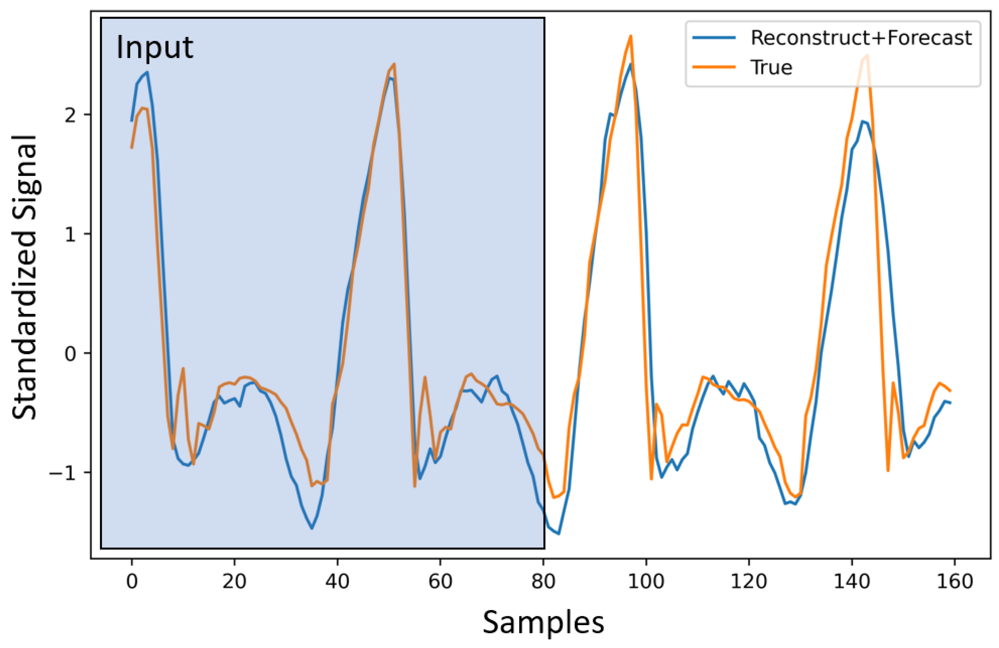
In this section, we provide results comparing the use of one-hot encoding vs. Gaussian encoding for the phase. We focus on the forecast task for simplicity. For this experiment, we pick the best and ( and ) via cross-validation for the M1 (i.e., the first model for h specified in Equation (6)), and apply them to M2. Although these parameters are not optimal for the M2, as shown in Table 1, it still outperforms M1. Our choice of s ensures that we obtain a forecast for 2 s. However, it is still useful to compare the results for the first 1 s of the forecast, compared to the overall forecast. This gives us an idea of how much error is built up over time. In Table 1, we show model performance for the 1 s and 2 s windows. Here, we use both versions of the modeling scheme for h (M1 and M2). These experiments are performed to find the best candidate for h, which properly models the phase and helps with performance improvement. The selected model is utilized for multi-task learning in the subsequent section. We report the RMSE (root mean square error) with encoding and without encoding. In Table 1, we can clearly see the performance boost that the model gains by adding the encoded phase information. As mentioned earlier, Gaussian encoding provides an overall improvement in performance. Hence, we choose the second model from this point on for the rest of the experiments. We also provide the detailed RMSE for each terrain for both encodings in Table 2. In Figure 4, we show a sample with the corresponding signal input, reconstruction, and prediction for these experiments.

Table 1.
RMSE report for different setup. First and second rows show the RMSE for 1 s and 2 s forecasting using the first model (M1) for h. Third and fourth rows correspond to the second model (M2) for h. The columns show the type of encoding that is used.
Table 2.
RMSE report for different terrains using M2.
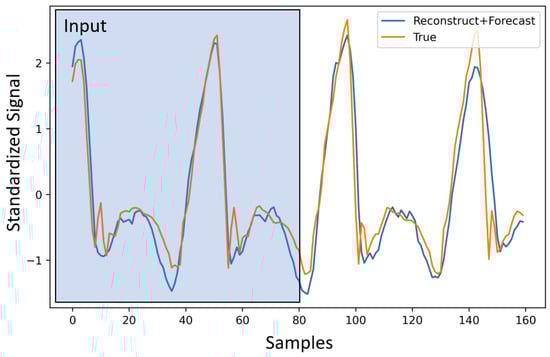
Figure 4.
Forecasting for IMU signals. The first 80 samples (2 s) are given to the model as an input. The reconstructed signal consists of the first 80 samples, and the forecasted signal is the last 80.
3.4. Relationship between and for Gait Task
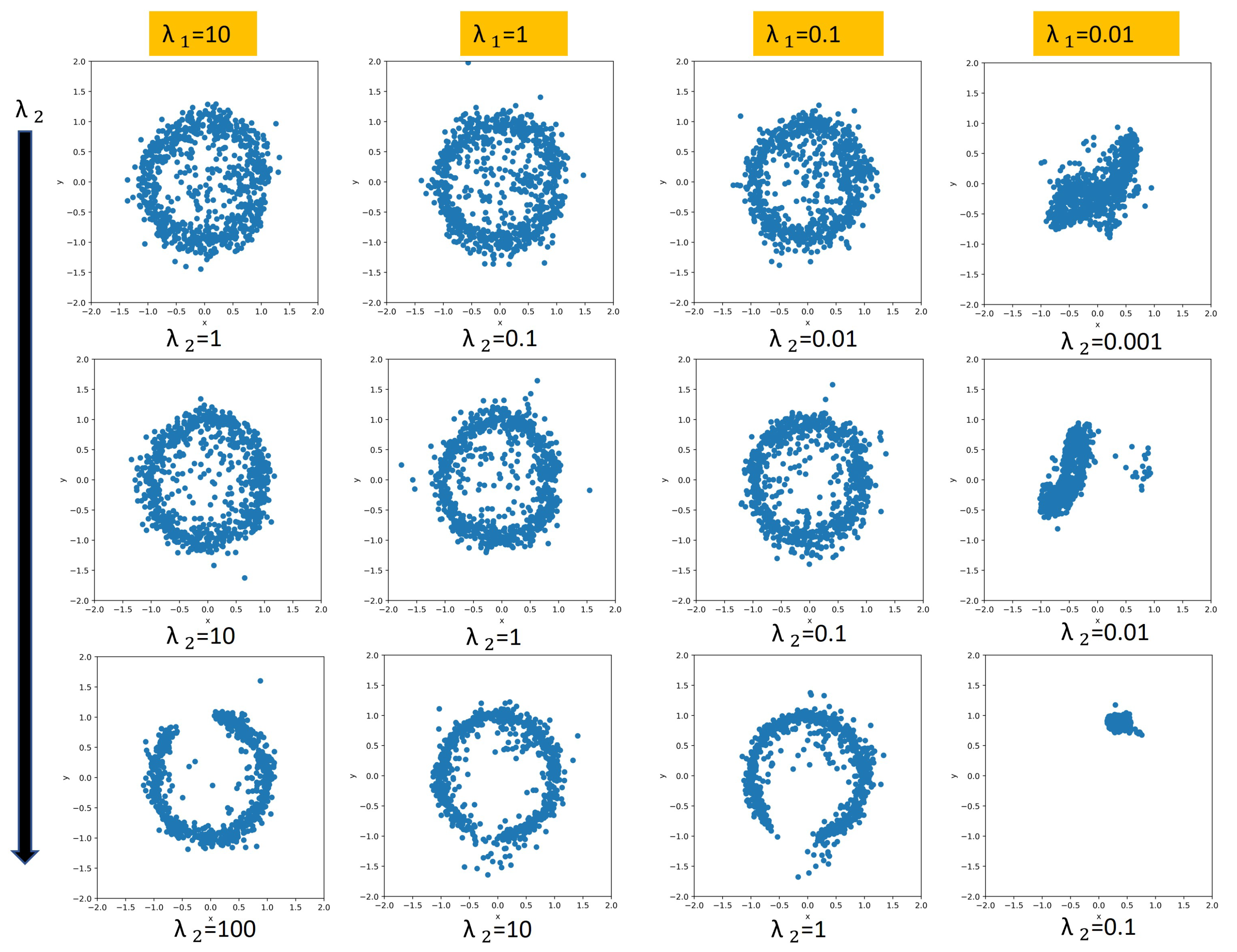
When we were exploring the relationship between the regularization coefficients, we noticed three different patterns based on the ratio given that the s are large enough. If the s are too small, then regularization does not impose any structure on the model. As a reminder, we represent the phase information in the latent space using two components, which correspond to the sine and cosine components of the phase. If phases are reconstructed perfectly, we will have a perfect circle for the latent space. The purpose of exploring the relationship between and is to find which values result in a fully learned phase regime. When the ratio is greater than 1, the projected phase in the latent space will look like a full circle, which indicates that the continuous transitions in a periodic gait cycle are captured. When the fraction is equal to 1, the structure is still captured, but it is not as prominent. If the ratio is less than one, the projected phase either forms an incomplete circle (i.e., it does not learn an interpretable structure that captures the periodic gait cycle) or some other shape. We show some of these patterns in Figure 5. The interpretability induced by these coefficients will help us with synthetic signal generation for IMU signals (see Section 3.6). It should be mentioned that the most interpretable architectures do not yield the best performance. This trade-off is expected. If we use bigger and values, then we are enforcing more structure, which results in loss of performance on the inference tasks. In our cases, the best-performing models do have a nice full circle latent space structure.
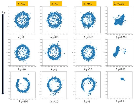
Figure 5.
Showing different variants for . Each plot is within the range [−2,2] for both x and y axis. The rows (from top to bottom) refers to the ratio being greater than one, equal to one and less than one respectively. Note that the full cyclic structure is not captured for . The last column does not capture the desired structure due to a low magnitude on the regularization weights.
3.5. Multi-Task Learning for Gait Task
In this section, we fully explore the different combinations of loss functions in Equation (4). The results are shown in Table 3. The left-hand side of the table indicates which loss function is used in the modeling, and the right-hand side shows the different metrics for model evaluation. and indicate whether we are doing classification for (i.e., the portion of data that we have as input), for (i.e., the portion of data that we do forecast for), or both. We use the following metrics: RMSE (for the whole window, the first half which corresponds to reconstruction; the second half which is forecasting), sMAPE (forecasting), MAE (forecasting), and f1-score (whole window). All the metrics are defined in Appendix A.1. In all the experiments (except the first one), the model includes reconstruction losses and regularization losses in the latent space. We also use one-hot encoding for convenience and select the second modeling scheme (M2) with a small network for h due to its better capacity and performance. All the weights in these experiments are fixed for fair comparison. The first row in Table 3 serves as the baseline for model performance.
Table 3.
Multi-task performance comparison. “√” represents the loss terms included in the training and “×” represents the ones that are absent in the training process.
Impact of Regularization. Comparing the first row against the fifth row, we observe some improvement in RMSE for the forecasting portion. Remember that the phase regularization is mainly imposing structure on the model for interpretability, which may not necessarily help with model performance. The results are very close, which shows that the additional regularization did not sacrifice performance.
Impact on Classification. When classification is considered, we observe a higher f1-score when including and . This is observed for both cases: without (rows 2–4) and with (rows 6–8) the forecasting portion. The highest overall performance is obtained when forecasting is also included (row 8).
Impact on Forecasting. When considering the case when forecasting is included (rows 5–8), we observe that all models with some classification (rows 6–8) have a lower than the base model (row 1) without classification. The best performance is obtained if only the term is included (row 6). However, the best is obtained by the model with all classification tasks included (row 8). Remember that this model also provided much higher performance for classification. This indicates a small trade-off between classification and forecasting tasks, but an overall boost in performance when considering them jointly.
Based on the experiments in Table 3, we can conclude that the multi-task learning indeed helped with model performance. In our case, it helped both with the f1-score and other metrics in the table.
3.6. Gait Signal Generation
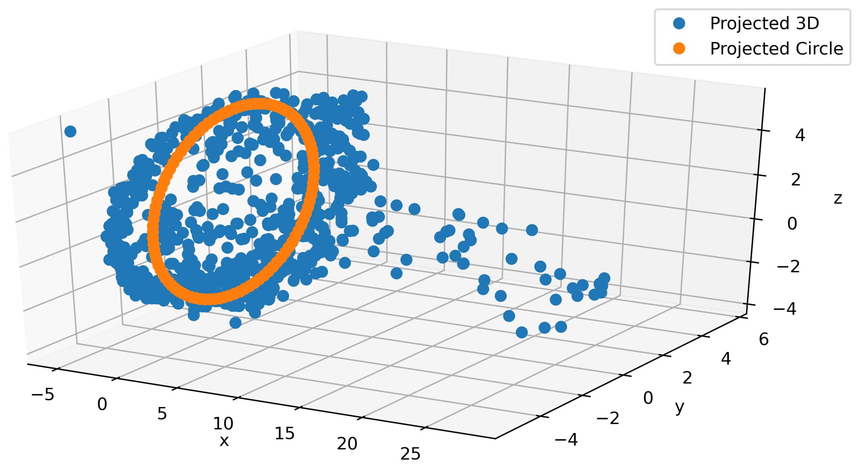
As part of the main contributions of this paper, we propose a model to generate realistic IMU signals which properly construct a continuous and smooth times series. For that purpose, we leveraged the interpretability of the latent space that we imposed. In Figure 6, a typical projection of the latent space into a 3-dimensional space using PCA is depicted. From the figure, we can observe that the plot consists of a circular shape and a tail (blue). Since these data correspond to walking on different terrains, we know the most important part of the signal should lie in the circular region. Building on that intuition, we ignore the tail and directly used the circular part. We postulate that even this circular region can be mapped to something even simpler by considering a single circular trajectory. A least squares approach is used to fit the circle (orange) to the PCA output as shown in Figure 6. By using the PCA’s inverse transform, we project back the circle to the proper dimension for the latent space and feed the output to the decoder to generate the IMU signals. In Appendix A.3, we provide a couple of snapshots of this procedure to show how smooth this data generation is. We can use this signal generation for augmentation to alleviate the cost of data collection. An animation is provided in the supplementary material.
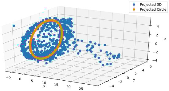
Figure 6.
Fitting a circle in 3D on the circular part of the latent space PCA projection.
3.7. ECG Forecasting
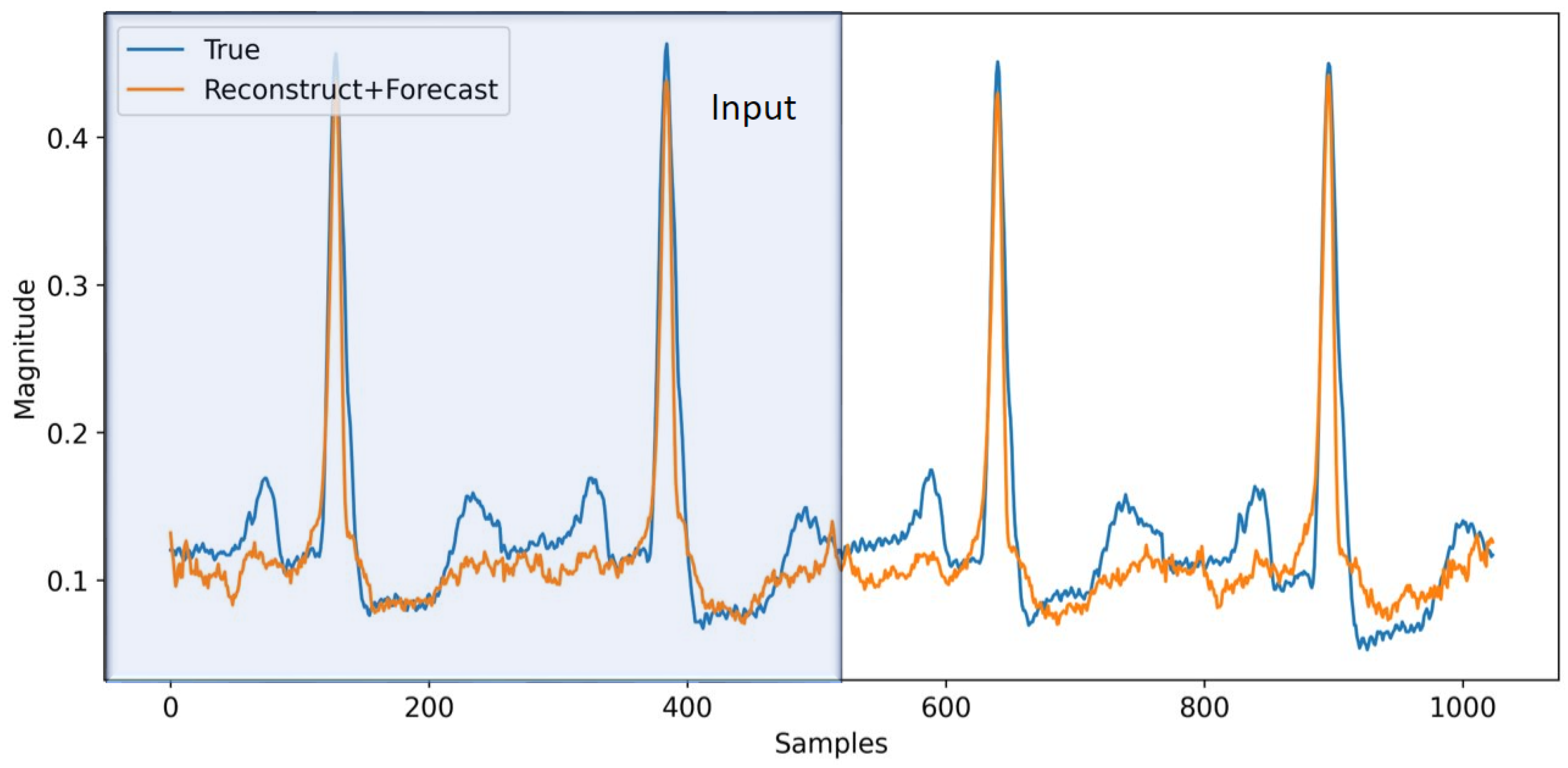
As an extension, in this section, we apply the aforementioned techniques to ECG signals from the MIT-BIH dataset [22]. We use bandpass filtering and normalization (re-scaling the data to be in [−1, 1] range) on the data to make it less noisy and also partition all the data into windows with length 1024 samples, which correspond to 4 s worth of data (i.e., s). With some minor adjustments to the model architecture and using one-hot encoding with the second model for h (M2), we train the model on this dataset to perform multi-task learning. The input to the model is half of the window (512 samples), and we forecast the next 512 samples. In Figure 7, a sample from the model is depicted. The model reasonably follows the trend for the ECG signal. The trend could have been improved if we had more data. The MIT-BIH dataset set is relatively small, making it difficult to model all the variations reliably. In Table 4, we providethe model performance for this dataset on multi-task learning. As before, the first row corresponds to pure reconstruction and forecasting without phase regularization and classification, which will serve as the baseline for the other experiments. In the fifth row, we add phase regularization to the model. We can clearly observe the improvement throughout all the metrics compared to the baseline. From the second through fourth rows, we are adding classification for both reconstruction and forecasting individually and combined. In all cases, the model’s performance is improved. In the sixth row, we combine phase regularization with classification for the forecasting portion. This combination results in the best performance in the RMSE total. As expected, multi-task learning helps with performance improvement compared to the baseline in all cases. Although the focus of this paper is on total RMSE as the performance metric, we can also see improvement in F1 scores in the different model combinations. We can conclude that phase information and regularization help the model performance by a respectable margin. On top of that, adding classification helps the model to improve even further. It should be mentioned that the model successfully recovers the QRS section of the signals, while it has difficulty capturing the (P, T) pair. This can be related to the reconstruction loss, which is more biased to reconstruct more prominent parts of the signals (QRS). Perhaps by applying some weight on the reconstruction loss we can improve the model performance on (P, T) pair, which is worth exploring in future work to resolve this issue.
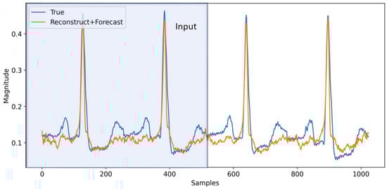
Figure 7.
Forecasting for ECG signals. The first 512 samples (2 s) are used as an input to the model and for the reconstruction task, while the second half of the signal is predicted by the model for forecasting.
Table 4.
Multi-task performance for ECG dataset. “√” represents the loss terms included in the training and “×” represents the ones that are absent in the training process.
4. Discussion
Throughout this work, we studied the effects of phase information and multi-task learning on the modeling of periodic signals. We started by incorporating phase into the model in two ways: (1) as an 8-dimensional vector to be concatenated to the input, and (2) in the latent space to add some structure to the model to help us with the interpretability of the model for signal forecasting and generation. In the first case, we clearly observed the benefit of using both phase information and multi-tasking. In the second case, as shown in Section 3.6, we can find a 3D plane to which we can project a circle and reliably generate new sequences, given that the model properly learns the phase information. Using this technique, we can generate synthetic data reliably in cases where data are difficult to acquire from patients. We also extended our work to ECG signals. In Table 4, we can observe the impact of the modeling on the MIT-BIH dataset. We analyzed the model performance in detail in Section 3.7. It is worth mentioning that modeling both datasets was challenging, but the MIT-BIH dataset was more difficult due to the low number of samples, which made it difficult to properly capture the underlying uncertainties and dynamics.
5. Conclusions
In this paper, we were able to boost model performance by incorporating phase information and multi-task learning. Our formulation and modeling allowed us to build a phase-based interpretable unit, which enabled us to gain some insight into the signal behavior. This insight resulted in reliable signal generation for sensory data. Overall, our scheme can be used in a medical settings, where periodic (e.g., ECG) signals are available. This scheme can help with predicting heart disease-related problems in advance. Due to the interpretable and reliable signal generation that our modeling offers, this method can be used as a synthetic generator in cases where data are scarce or acquiring new data is very expensive.
For future work, in order to overcome some of the difficulties related to data scarcity and modeling, we are planning to use transfer learning techniques to leverage training on larger, more general datasets to improve results on the smaller datasets related to our application. It should also be mentioned that the aforementioned techniques and methodology can be applied to any periodic signal. So, another direction would be to extend our model to any signal with a certain periodic behavior.
Supplementary Materials
The following supporting information can be downloaded at: https://www.mdpi.com/article/10.3390/info13070326/s1.
Author Contributions
Conceptualization, R.S., E.L.; methodology, R.S., E.L.; software, R.S.; validation, R.S.; formal analysis, R.S., E.L.; resources, R.S.; data curation, R.S.; writing—original draft preparation, R.S.; writing—review and editing, R.S., E.L.; supervision, E.L. All authors have read and agreed to the published version of the manuscript.
Funding
This work is supported by the National Science Foundation (NSF) under awards CNS 1552828 and IIS 2037328.
Institutional Review Board Statement
Not applicable.
Informed Consent Statement
Not applicable.
Data Availability Statement
Not applicable.
Conflicts of Interest
The authors declare no conflict of interest.
Appendix A
Appendix A.1. Metric Definition
In the section, we define the evaluation metric that we used in the experiment section. Here X, Y are row vectors for convenience where they belong to . The metrics are defined as follows:
where is the norm operator and , , and refer to true positive, false positive, and false negative, respectively.
Appendix A.2. Model Architecture
In this section, we describe all the models in detail. In Figure A1, the model for the first setup where the phase is part of the latent space has been described. We provided all the details. Norm in the network refers to group norm in Pytorch. In Figure A2, we show the architecture for the the ODE-net, phase network, and the classifier. We can clearly see the difference between this model and the first one. We have more flexibility and capacity to model the complex signals. In Figure A2, we show the down sampling and the decoder for the second modeling scheme. This summarizes all of the modeling architecture that we described in the multi-task section.
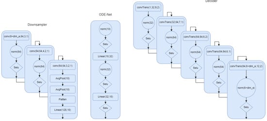
Figure A1.
Down sampler and decoder for model 1. is 8 if we use encoding.
Figure A1.
Down sampler and decoder for model 1. is 8 if we use encoding.
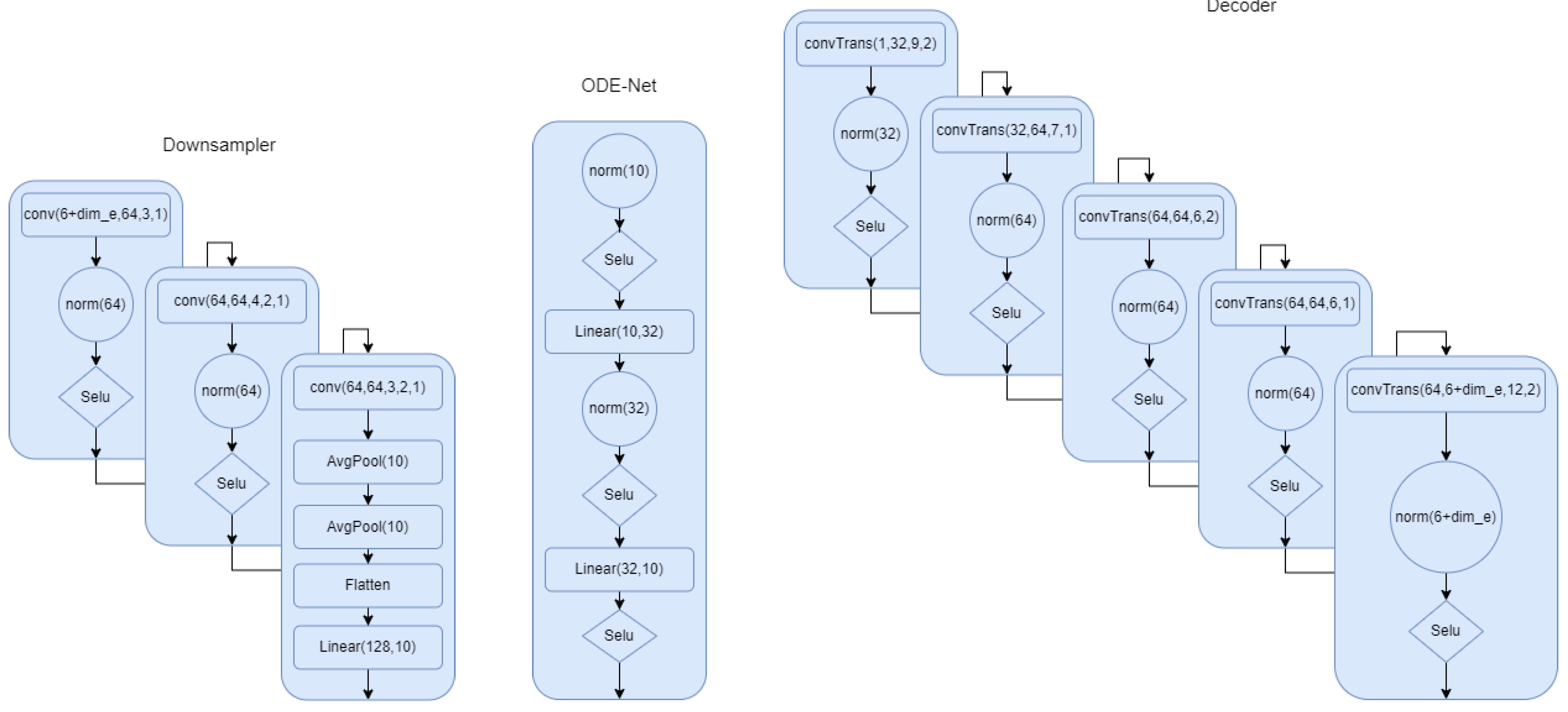
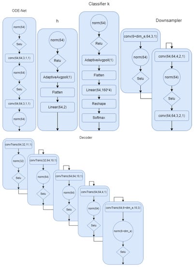
Figure A2.
Down sampler and decoder for model 2. is 8 if we use encoding.
Figure A2.
Down sampler and decoder for model 2. is 8 if we use encoding.

Appendix A.3. IMU Generation
In Figure A3, we can observe how the sequence of the IMU signals is generated. By generating this synthetic data with the projected circle, we can argue there is a lot of redundancy in the data. The tail in Figure 6 seems to be the result of the uncertainty in data collection. So, just by having the phase incorporated into the model, not only we provide interpretability for the model, but also, we are able to reliably generate synthetic data. The spike-like points in the signal generation in couple of snapshots is very common in the actual data. So, it is not surprising that they appear in the data generation.
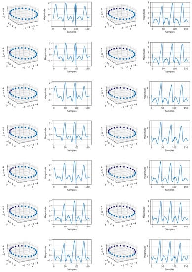
Figure A3.
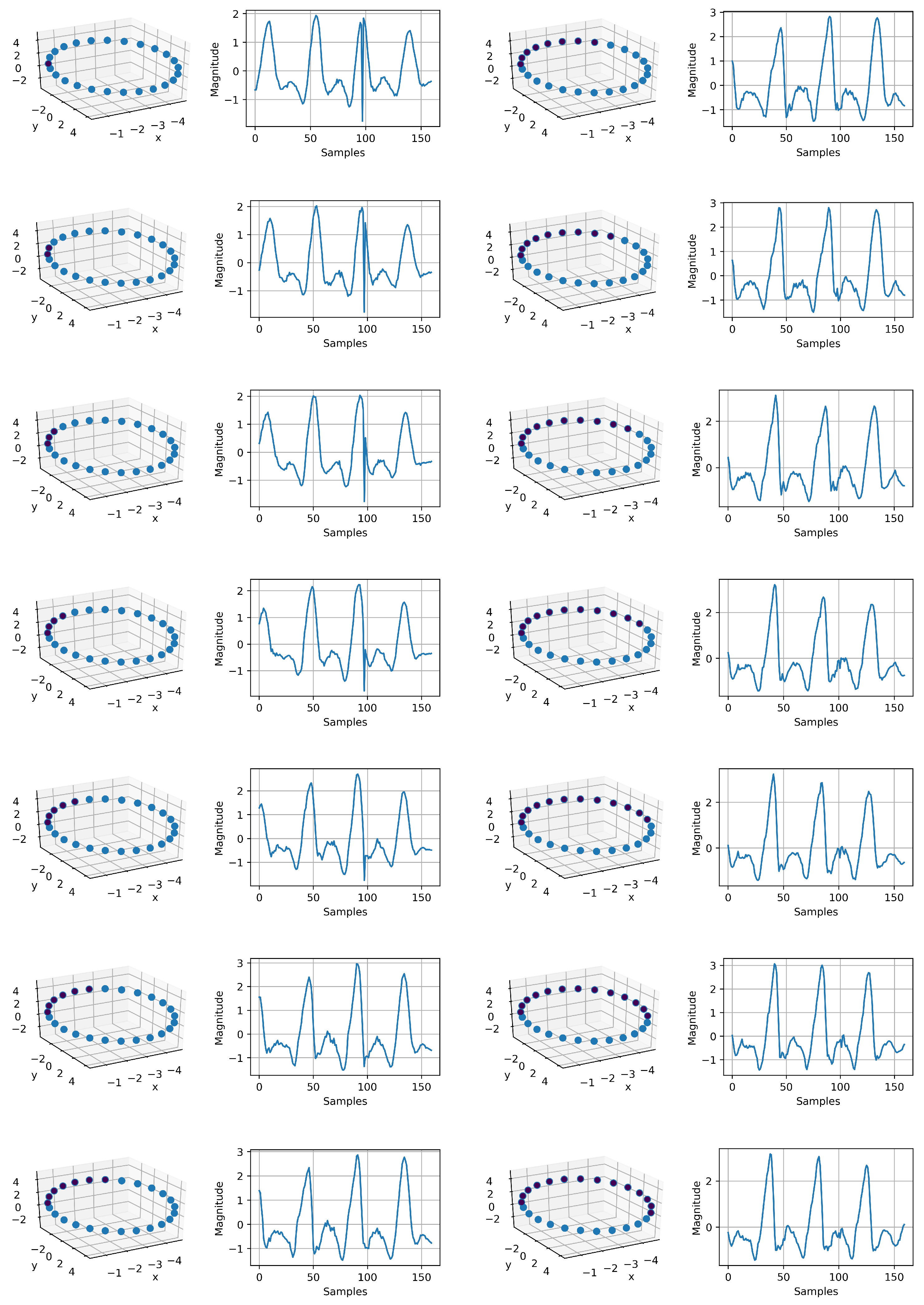
IMU signal generation using the mapped circle in 3D space. Each point on the circle corresponds to a time series. In total, we have 14 sequence, which are sequentially related. This shows that our intuition about the phase information is valid. Just by having the mapped circle, as it can be observed, we successfully generated a continuous time variant IMU signal. The resolution can be increased, and it depends on the number samples on the mapped circle. This signal generation can be used for augmentation to compensate for data imbalance. The sequence starts at the top of the first column to the bottom and continues to the top of the second column to the bottom.
Figure A3.
IMU signal generation using the mapped circle in 3D space. Each point on the circle corresponds to a time series. In total, we have 14 sequence, which are sequentially related. This shows that our intuition about the phase information is valid. Just by having the mapped circle, as it can be observed, we successfully generated a continuous time variant IMU signal. The resolution can be increased, and it depends on the number samples on the mapped circle. This signal generation can be used for augmentation to compensate for data imbalance. The sequence starts at the top of the first column to the bottom and continues to the top of the second column to the bottom.
References
- Dama, F.; Sinoquet, C. Analysis and modeling to forecast in time series: A systematic review. arXiv 2021, arXiv:2104.00164. [Google Scholar]
- Fawaz, H.I.; Forestier, G.; Weber, J.; Idoumghar, L.; Muller, P.A. Deep learning for time series classification: A review. Data Min. Knowl. Discov. 2019, 33, 917–963. [Google Scholar] [CrossRef] [Green Version]
- Song, H.; Rajan, D.; Thiagarajan, J.; Spanias, A. Attend and diagnose: Clinical time series analysis using attention models. In Proceedings of the Thirty-Second AAAI Conference on Artificial Intelligence, New Orleans, LA, USA, 2–7 February 2018. [Google Scholar]
- Harutyunyan, H.; Khachatrian, H.; Kale, D.C.; Steeg, G.V.; Galstyan, A. Multitask learning and benchmarking with clinical time series data. Sci. Data 2019, 6, 1–18. [Google Scholar] [CrossRef] [PubMed] [Green Version]
- Jadon, S.; Milczek, J.K.; Patankar, A. Challenges and approaches to time-series forecasting in data center telemetry: A Survey. arXiv 2021, arXiv:2101.04224. [Google Scholar]
- Karim, F.; Majumdar, S.; Darabi, H.; Chen, S. LSTM fully convolutional networks for time series classification. IEEE Access 2018, 6, 1662–1669. [Google Scholar] [CrossRef]
- Nakano, K.; Chakraborty, B. Effect of Data Representation for Time Series Classification—A Comparative Study and a New Proposal. Mach. Learn. Knowl. Extr. 2019, 1, 1100–1120. [Google Scholar] [CrossRef] [Green Version]
- Elsayed, N.; Maida, A.; Bayoumi, M.A. Gated Recurrent Neural Networks Empirical Utilization for Time Series Classification. In Proceedings of the 2019 International Conference on Internet of Things (iThings) and IEEE Green Computing and Communications (GreenCom) and IEEE Cyber, Physical and Social Computing (CPSCom) and IEEE Smart Data (SmartData), Atlanta, GA, USA, 14–17 July 2019; pp. 1207–1210. [Google Scholar]
- Thomsen, J.; Sletfjerding, M.B.; Stella, S.; Paul, B.; Jensen, S.B.; Malle, M.G.; Montoya, G.; Petersen, T.C.; Hatzakis, N.S. DeepFRET: Rapid and automated single molecule FRET data classification using deep learning. bioRxiv 2020. [Google Scholar] [CrossRef] [PubMed]
- Shih, S.Y.; Sun, F.K.; Lee, H.y. Temporal pattern attention for multivariate time series forecasting. Mach. Learn. 2019, 108, 1421–1441. [Google Scholar] [CrossRef] [Green Version]
- Zhou, H.; Zhang, S.; Peng, J.; Zhang, S.; Li, J.; Xiong, H.; Zhang, W. Informer: Beyond efficient transformer for long sequence time-series forecasting. In Proceedings of the Thirty-Fifth AAAI Conference on Artificial Intelligence, Virtual Conference, 2–9 February 2021. [Google Scholar]
- Chen, R.T.Q.; Rubanova, Y.; Bettencourt, J.; Duvenaud, D. Neural Ordinary Differential Equations. Adv. Neural Inf. Process. Syst. 2018, 31, 6571–6583. [Google Scholar]
- Chen, R.T.Q.; Amos, B.; Nickel, M. Learning Neural Event Functions for Ordinary Differential Equations. arXiv 2021, arXiv:2011.03902. [Google Scholar]
- Ribeiro, M.T.; Singh, S.; Guestrin, C. “ Why should i trust you?” Explaining the predictions of any classifier. In Proceedings of the 22nd ACM SIGKDD International Conference on Knowledge Discovery and Data Mining, San Francisco, CA, USA, 13–17 August 2016; pp. 1135–1144. [Google Scholar]
- Chen, C.; Li, O.; Tao, C.; Barnett, A.J.; Su, J.; Rudin, C. This looks like that: Deep learning for interpretable image recognition. arXiv 2018, arXiv:1806.10574. [Google Scholar]
- Sun, X.; Yang, D.; Li, X.; Zhang, T.; Meng, Y.; Han, Q.; Wang, G.; Hovy, E.; Li, J. Interpreting Deep Learning Models in Natural Language Processing: A Review. arXiv 2021, arXiv:2110.10470. [Google Scholar]
- Oreshkin, B.N.; Carpov, D.; Chapados, N.; Bengio, Y. N-BEATS: Neural basis expansion analysis for interpretable time series forecasting. arXiv 2019, arXiv:1905.10437. [Google Scholar]
- Lim, B.; Arık, S.Ö.; Loeff, N.; Pfister, T. Temporal fusion transformers for interpretable multi-horizon time series forecasting. Int. J. Forecast. 2021, 37, 1748–1764. [Google Scholar] [CrossRef]
- Zhong, B.; da Silva, R.L.; Tran, M.; Huang, H.; Lobaton, E. Efficient Environmental Context Prediction for Lower Limb Prostheses. IEEE Trans. Syst. Man Cybern. Syst. 2021, 52, 3980–3994. [Google Scholar] [CrossRef]
- Zhou, X.; Wang, D.; Krähenbühl, P. Objects as points. arXiv 2019, arXiv:1904.07850. [Google Scholar]
- Cramér, H.; Wold, H. Some theorems on distribution functions. J. Lond. Math. Soc. 1936, 1, 290–294. [Google Scholar] [CrossRef]
- Moody, G.B. The impact of the MIT-BIH Arrhythmia Database. IEEE Eng. Med. Biol. 2001, 20, 45–50. [Google Scholar] [CrossRef] [PubMed]
- Available online: https://tsaug.readthedocs.io/en/stable/quickstart.html (accessed on 22 June 2022).
- Available online: https://github.com/ARoS-NCSU/PhysSignals-InterpretableInference (accessed on 22 June 2022).
- Loshchilov, I.; Hutter, F. Fixing Weight Decay Regularization in Adam. arXiv 2018, arXiv:1711.05101. Available online: https://openreview.net/forum?id=rk6qdGgCZ (accessed on 22 June 2022).
- Hinton, G. Coursera Neural Networks for Machine Learning Lecture 6. 2018. Available online: http://www.cs.toronto.edu/~hinton/coursera/lecture6/lec6.pdf (accessed on 22 June 2022).
Publisher’s Note: MDPI stays neutral with regard to jurisdictional claims in published maps and institutional affiliations. |
© 2022 by the authors. Licensee MDPI, Basel, Switzerland. This article is an open access article distributed under the terms and conditions of the Creative Commons Attribution (CC BY) license (https://creativecommons.org/licenses/by/4.0/).