A Forward-Looking Approach to Compare Ranking Methods for Sports

Abstract

In this paper, we provide a simple forward-looking approach to compare rating methods with respect to their stability over time. Given a rating vector of entities involved in the comparison and a ranking indicated by the rating, the stability of the methods is measured by the change in rating vector and ranks of the entities over time from a forward-looking perspective. We investigate various linear algebraic rating methods and use the Euclidean distance and Kendall tau rank correlation to measure their stability in rating and ranking, respectively. The investigations are based on both rolling and expanding window approaches. We apply the methodology to sports as a widely known ranking and rating environment. The results suggest that PageRank and Massey rating methods provide better rating and ranking stability than simple methods, such as winning percentage, and more advanced ones, such as Colley’s least square and Keener’s eigenvector-based method. Finally, a simple way to examine the potential predictive power of the rating methods is also provided.

1. Introduction

Rating items is a fundamental task that aims at providing a ranking and making decisions according to it. For instance, in sports, the ranking of players or teams is provided by some scoring system, such as ‘three points for a win and one for the draw’ in soccer, or more complex systems such as Élő in chess or ATP ranking in men’s tennis. For a good book on ratings in sports, see, e.g., [1].

Many different rating methods have been developed, and all of them are based on some assumptions or formal axioms that have to be satisfied by the rating; see, e.g., [2,3,4,5]. In the case of sports, rating methods are also considered as key elements of making single-game outcome predictions; see, e.g., [6].

Although the literature on rating and rating-based predictions in sports is vast, only a few papers can be found that address the problem of evaluating and comparing the stability and robustness of rating methods over a season in a round robin-like system, such as soccer or US major sports. For some related papers, see, e.g., [5,7,8]. Our study, however, is different from the above ones, as outlined in the following paragraph.

The paper [5] focuses on the general properties of sport ranking including Colley, Win-loss, Elo, and Markov methods. The authors evaluate the ranking of these methods in relation to properties such as Opponent Strength, Incentive to Win and Sequence of Matches. In our case, we propose a new comparison method based on a forward-looking approach to evaluate the ranking and rating stability of selected common ranking methods. In [7], the authors empirically evaluate the predictive power of eight sports ranking methods. Although we evaluated similar ranking methods such as PageRank, Winning Pacentage, Rating Percentage Index, and Keener, our comparison approach is different mainly by the stability measures using forward-looking approach. Our investigations may be considered as a meta analysis for predictive power studies: we hypothesize that there is a relation between predictive power and stability/robustness, and we consider our study as an initial step in this direction. Finally, in [8], the authors focus on the analysis of the sensitivity measure of the rating vectors of three linear-algebra-based ranking methods including Colley, Massey, and Markov methods. The authors employ reverse engineering of a simple input ranking vector that they use to build a perfect season to determine the output rating vectors produced by the three methods to measure the sensitivity. This is also a different technique from our approach.

The stability problem has also been addressed in the literature of network science, especially in the case of centrality measures; see, e.g., [9,10,11]. Since many rating methods can be interpreted as network centrality measures, investigating the stability problem for ratings in the sport domain is a convenient next step in this direction.

In this study, we propose a simple forward-looking approach to actively compare rating and ranking methods with respect to their robustness and stability over time. Informally, a rating (or ranking) method is considered to be stable over time if the differences between the rating (or ranking) vectors obtained for the consecutive time periods are steadily small, using proper functions to calculate the difference. Our approach is a forward-looking one in the sense that stability is measured from a future perspective: if a rating ‘at present’ is closer to the rating obtained at some future time point, this indicates stability. This study attempts to evaluate and compare ratings and rankings by dynamically modifying the dataset (used to calculate ratings) using rolling and expanding window simulations, respectively.

The rest of this paper is organized as follows: In Section 2, we formally discuss several commonly used rating and ranking methods that we use in our simulations. In Section 3, we describe the evaluation framework and comparison methods. In Section 4, we discuss the simulations results on some European football league datasets. Finally, we conclude and address some future research directions in Section 5.

2. Rating and Ranking Methods

In this section, we give a short description of the ranking methods we will use. For a more detailed introduction about ranking methods, refer to [12,13].

Let $V=(1,\dots ,n)$ be the set of n teams to be rated, and let R be the number of rounds in a competition among the teams in V. After round r ($r=1,\dots ,R$), a rating function ${\varphi }^r:V\to \mathbb{R}$ assigns a score to each team which we may call their quantitative ‘strength’. A ranking ${\sigma }^r:V\to V$ is an ordering of the teams simply obtained from a rating on V by a proper sorting. For rating the teams, we consider only the final scores of the games played.

We define the $n\times n$ matrices W and D as

$$W_{ij}=\#\left\{i\mathrm{won}\mathrm{against}j\right\},$$

and

$$D_{ij}=\#\left\{\mathrm{draws}\mathrm{between}i\mathrm{and}j\right\}.$$

The score matrix $S\in {\mathbb{R}}^{n\times n}$ is defined as

$$S_{ij}=\#\left\{\mathrm{points}i\mathrm{scored}\mathrm{against}j\right\}.$$

To avoid fully zero rows in S, we consider $S_{ij}=S_{ji}=1/2$ if the outcome of the game is 0:0.

Using W matrix, the elements of the vectors $\mathbf{w}=W\mathbf{1}$, $\mathbf{l}=W^t\mathbf{1}$, $\mathbf{d}=D\mathbf{1}$, and $\mathbf{t}=(W+W^t+D)\mathbf{1}$ are the number of wins, loses, draws, and total number of games played by team i ($i=1\dots ,n$), respectively, where $\mathbf{1}$ is the n-element vector with all entries being one. Since each game is either a win, a lose, or a draw, $\mathbf{t}=\mathbf{w}+\mathbf{l}+\mathbf{d}$. We define $T=\mathrm{diag}\left(t_i\right)$, which is the diagonal matrix with entries $T_{ii}=t_i$ and $T_{ij}=0$, if $i\ne j$ ($i,j=1\dots ,n$). Similarly, we may define the vectors $\mathbf{s}=S\mathbf{1}$, $\mathbf{u}=S^t\mathbf{1}$ as the total number of scores by team i against the opponents and by the opponents against team i, respectively.

2.1. Winning Percentage (WP)

The winning percentage of team i after round r is simply defined as ${\varphi }_{WP}^r\left(i\right)=(w_i+\kappa d_i)/t_i$, where $\kappa$ is a parameter between 0 and 1 and can be interpreted as the ‘value’ of a draw. For example, if we take $\kappa =1/3$, it refers to the fact that the value of a draw is one third of the value of a win. The vector of winning percentages after round r can be computed as

$${\varphi }_{WP}^r=T^{-1}(\mathbf{w}+\kappa \mathbf{d}).$$

By considering the score matrix S, a similar quantity can be calculated as ${\varphi }_{WP\left(S\right)}^r=T^{-1}\mathbf{s}.$

Observe that this method does not take into consideration the strength of the opponent teams; only the outcome games count.

2.2. Rating Percentage Index (RPI)

The Rating Percentage Index takes into account the WP of the team’s opponents and the WP of their opponents’ opponents [14]. The average winning percentage of team i’s opponents after round r is calculated as

$$\frac{1}{t_i}\sum _j(W_{ij}+W_{ji}+D_{ij}){\varphi }_{WP}^r\left(j\right),$$

where the average is taken over the set of the team’s previous opponents after round r. The vector of the average opponents’ winning percentages is $T^{-1}(W+W^t+D){\varphi }_{WP}^r$. The winning percentages of the opponents’ opponents can be calculated as $T^{-1}{(W+W^t+D)}^2{\varphi }_{WP}^r$. After round r, RPI vector is calculated as the following weighted average:

$${\varphi }_{RPI}^r=\frac{1}{4}{\varphi }_{WP}^r+\frac{1}{2}{T}^{-1}(W+W^t+D){\varphi }_{WP}^r+\frac{1}{4}{T}^{-1}{(W+W^t+D)}^2{\varphi }_{WP}^r,$$

and similarly, given score matrix S, as

$${\varphi }_{RPI}^r=\frac{1}{4}{\varphi }_{WP\left(S\right)}^r+\frac{1}{2}{T}^{-1}(S+S^t){\varphi }_{WP\left(S\right)}^r+\frac{1}{4}{T}^{-1}{(S+S^t)}^2{\varphi }_{WP\left(S\right)}^r.$$

2.3. Massey’s Least Squares Method (M)

The only statistics used in Massey’s least squares method [15] are the number of wins and losses for each team. The rating ${\varphi }_M^r$ of the teams after round r is obtained by the solution of the linear system

$$M{\varphi }_M^r=\mathbf{w}-\mathbf{l},$$

where $M=T-W-W^t-D$ contains the total number of games played by the teams in the diagonal, while $M_{ij}$ is $-1$ times the number of games played between teams i and j, $i\ne j$. The method naturally incorporates draws, since a draw between two teams increases $M_{ij}$ and $M_{ji}$ by one, while the right-hand side $\mathbf{w}-\mathbf{l}$ remains unchanged. Since $rank\left(M\right)<n$, the linear system does not have a unique solution. To handle this problem, one possible solution is to replace any row in M with $\mathbf{1}$ and the corresponding entry of $\mathbf{w}-\mathbf{l}$ with zero.

2.4. Colley’s Least Squares Method (C)

The Colley method is also a modification of the least squares method utilizing an observation called Laplace’s rule of succession (see [16], p. 148), which states that if one observed k successes out of m attempts, then $(k+1)/(m+1)$ is a better estimate for the next event to be a success than $k/m$. The rating vector ${\varphi }_C^r$ of the teams is the solution of the linear system

$$C{\varphi }_C^r=\mathbf{b},$$

where $C=M+2I$ (here, I is the identity matrix) and $\mathbf{b}=\mathbf{1}+1/2(\mathbf{w}-\mathbf{l})$. It can be proved that the linear system has a unique solution.

2.5. Keener Method (K)

Keener’s method [17] is a so-called spectral rating method which uses the Perron–Frobenius eigenvector for the rating, and (after round r) it is given by the solution of the eigenvalue equation

$$T^{-1}(W+\kappa D){\varphi }_K^r=\lambda {\varphi }_K^r,$$

where $\lambda$ is the dominant eigenvalue of the matrix $T^{-1}(W+\kappa D)$, and it exists for a matrix with non-negative entries such that any other eigenvalue is smaller in absolute value. The corresponding eigenvector, called the Perron–Frobenius eigenvector, has non-negative entries and provides the rating of the teams. Originally, the method was defined for the case in which we consider the score matrix S. The Keener matrix, also based on the Laplace’s rule of succession, is defined as

$$K_{ij}=h\left(\frac{S_{ij}+1}{S_{ij}+S_{ji}+1}\right),$$

where h is a skewing function helping to reduce the difference between the upper and lower ends of the rating. We use the original function defined by Keener, namely,

$$h\left(x\right)=\frac{1}{2}+\frac{1}{2}\mathrm{sgn}(x-\frac{1}{2})\sqrt{|2x-1|}$$

The Keener rating vector ${\varphi }_{K\left(S\right)}^r$ of the teams is given by the solution of the equation

$$T^{-1}K{\varphi }_{K\left(S\right)}^r=\lambda {\varphi }_{K\left(S\right)}^r.$$

2.6. PageRank Method (PR)

The PageRank method [18] was originally designed to rank web pages based on their position in the WWW network. The idea behind it came from the basic properties of Markov chains (see, e.g., [12], Chapter 4). In the context of sports, the rating of the teams is calculated in an iterative way using the recursion formula

$$PR\left(i\right)=\frac{\lambda }{n}+(1-\lambda )\sum _{j\in N^{+}\left(i\right)}\frac{PR\left(j\right)}{w_j},$$

where $N^{+}\left(i\right)$ is the set of teams defeated by team i at least once, $w_j$ is the total number of wins of team j, and $\lambda \in [0,1]$ is a parameter (usually $0.1$ or $0.2$) to guarantee convergence.

To see the relationship between the PageRank formula and the theory of Markov chains, we may write the above equation in a vector equation form as

$$\mathbf{PR}=\frac{\lambda }{N}{[I-(1-\lambda )S{D}^{-1}]}^{-1}\mathbf{1},$$

where $\mathbf{PR}$ PageRank vector contains the PageRank values of each team, D is the diagonal matrix $D=\mathrm{diag}\left[{(D_{ii}={\sum }_{\ell =1}^n{S}_{i\ell })}_{i=1}^n\right)]$, while I is the $n\times n$ identity matrix. Assuming that $\mathbf{1}\mathbf{PR}=1$ implies that $\mathbf{PR}=M\mathbf{PR}$, with $M=\lambda /n\mathbf{1}{\mathbf{1}}^T-(1-\lambda )S{D}^{-1}$. This shows that $\mathbf{PR}$ is the eigenvector of matrix M for eigenvalue one, which is the largest eigenvalue of M as a consequence of the Perron–Frobenius theorem for row-stochastic matrices. The rating vector ${\varphi }_{PR\left(S\right)}^r$ of the teams after round r can be calculated using, for instance, the power iteration method.

2.7. Graph Representation of the Methods

We shall emphasize that all the above-defined methods have a graph theoretical interpretation. Using the game results data set, one can define a directed multigraph, where nodes represent players/teams, while edges between them represent outcomes of games they played. The edges are directed and each of them is going from the loser team to the winning team. If ties are also considered, they can be represented by two directed links with opposite directions and half or some fractional weight. In this case, matrix W is the adjacency matrix of the directed multigraph, and $\mathbf{w}$ and $\mathbf{l}$ contain the in- and out-degrees of nodes, respectively. From a network science perspective, Massey’s M matrix is the graph Laplacian if the result matrix is treated as the matrix of a symmetric undirected graph. The Massey rating vector ${\varphi }_M$ is then equivalent to the potential vector over a resistor network defined by W with supply vector $\mathbf{w}-\mathbf{l}$ [19]. The PageRank method is a simple modification of the classic PageRank algorithm, performed on the results graph.

3. Evaluation and Comparison of Rating Methods

In this section, we present the applied simulation approaches and the definitions of the stability of ratings and rankings as well as the rating error. To deal with the dynamic nature of sport competitions, we perform rolling window (RW) and expanding window (EW) simulations, described as follows.

3.1. Rolling Window Approach

Let $W^t$ (or $S_t$) be the results matrix generated just after t games (here $t=50,60,70,\dots$). Let ${\varphi }_{RW}^t$ be the rating vector after t games played. We generate the results matrix $W_{RW}^{\Delta t,t+\Delta t}$ with the fixed number of games (window length) $\Delta t$ and calculate the rating ${\varphi }_{RW}^{\Delta t,t+\Delta t}$ for the new matrix using the same rating method. For example, if $\Delta t=10$, then games from 1 to 50, 11 to 60, etc., are considered to create the results matrix and ratings.

3.2. Expanding Window Approach

In the expanding window case, let $W_{EW}^{(T,\Delta t)}$ (or $S_{EW}^{(T,\Delta t)}$) be the result matrix generated by an incremental number of games starting from the first T games with expansion factor $\Delta t$. For instance, if starting from $T=50$ with expansion factor $\Delta t=10$, then $W_{EW}^{(T,\Delta t=10)}$ is the result matrix generated considering the first 50, 60, 70, etc., games from the beginning of the competition. The team rating after game t is given by ${\varphi }_{EW}^t$.

3.3. Rating Stability

To measure the stability of the considered methods, we compute the Euclidean distance between consecutive rating vectors obtained by either the rolling or the expanding window approach with specified $\Delta t$ values [20]. Formally, we calculate

$$d_{RW}^2\left(t\right)=\left|\right|{\varphi }_{RW}^{(k\Delta t,t+\Delta t)}-{\varphi }_{RW}^t{\left)\right||}_2^2,$$

where $\left|\right|·{\left|\right|}_2$ denotes the Euclidean norm. If we average $d_{RW}^2\left(t\right)$ for all $t=50,60,\dots$ with $k=1,2,\dots$ we obtain a single value representing the average stability of the rating method over the whole competition or up to a given round. The stability in the case of the expanding window approach is measured similarly.

3.4. Ranking Stability

To measure the stability of rankings generated by the applied rating methods, we measure rank correlations using the Kendall tau method [21]. Given two consequtive rankings, ${\sigma }_{RW}^t={\sigma }^1$ and ${\sigma }_{RW}^{(t+\Delta t)}={\sigma }^2$, the Kendall tau distance is defined as

$${\tau }_{RW}^t=\frac{\#\left\{\mathrm{teams}(i,j):\left({\sigma }_i^1>{\sigma }_j^1\mathrm{and}{\sigma }_i^2<{\sigma }_j^2\right)\mathrm{or}\left({\sigma }_i^1<{\sigma }_j^1\mathrm{and}{\sigma }_i^2>{\sigma }_j^2\right)\right\}}{\frac{1}{2}n\left(n-1\right)}$$

where ${\sigma }_i^1$ and ${\sigma }_i^2$ is the rank of team i in ranking ${\sigma }_{RW}^t$ and ${\sigma }_{RW}^{(k\Delta t,t+\Delta t)}$ ($t=50,60,\dots$ with $k=1,2,\dots$), respectively.

We can average ${\tau }_{RW}^t$ for all $t=50,60,\dots$: we obtain a single value representing the mean stability of the ranking method over the whole competition or up to a given round. The stability in the case of the expanding window approach can be measured similarly.

3.5. Rating Error

We also estimate the potential predictive power of the rating methods in a simple way. Each dataset is divided into two subsets: a training set and a test set. For the training set, a rating ${\varphi }^t$ is calculated for t games ($t=50$ fixed in the case of rolling window approach, while $t=50,60,\dots$ in the case of the expanding window approach). The test set consists of the next $\Delta t$ games ($\Delta t=10$ in our simulations). We define the prediction error $E_{\varphi }^t$ of a rating method $\varphi$ as the proportion of games in the test set, such that the lower-rated team beat the higher-rated one, i.e.,

$$\begin{array}{cc}{E}_{\varphi }^t& =\frac{\#\left\{\mathrm{team}i\mathrm{beats}j\mathrm{in}\mathrm{test}\mathrm{set}\mathrm{and}{\varphi }_i<{\varphi }_j\right\}}{\#\left\{\mathrm{games}\mathrm{in}\mathrm{test}\mathrm{set}\right\}}\\ & +\frac{\#\left\{\mathrm{team}i\mathrm{and}j\mathrm{tie}\mathrm{in}\mathrm{dataset}t\mathrm{and}{\varphi }_i\ne {\varphi }_j\right\}}{\#\left\{\mathrm{games}\mathrm{in}\mathrm{test}\mathrm{set}\right\}}\end{array}$$

The total error is calculated as the average of the errors obtained for each train and test set sample.

4. Results

We performed our experiments using English Premier League Datasets (source: https://www.kaggle.com/datasets/saife245/english-premier-league (accessed on 15 March 2022)). The datasets contain the date of the game, the name of the teams, the home and away scores, and the total points of the teams during the competition. To generate the results matrices (graphs), we used W matrix in the case of PageRank, Massey, Colley, WP, and RPI methods. In the case of the Keener Method, we considered the Score matrix S. We performed rolling window (RW) and expanding window (EW) simulations to analyze the ranking and rating stability using the Kendall tau and Euclidean methods, respectively. The results are presented via tables and plots in this section.

4.1. Comparison of Top-5 Teams Ranking by Rolling Window Approach

First, we compared the rankings and ratings of the top-5 teams using our rolling window and expanding window approaches. Here, we considered standard deviation in rating the top-5 teams at different window times (games).

Table 1. Comparison of top-5 teams rate–rank by rolling window approach.

		10–60 Games			20–70 Games			30–80 Games
Method	Teams	Ranks	Rating	Teams	Ranks	Rating	Teams	Ranks	Rating
PageRank	‘Man. City’	1	0.0696	‘Man. City’	1	0.0894	‘Man. City’	1	0.0895
	‘Man. United’	2	0.0067	‘Arsenal’	2	0.0815	‘Arsenal’	2	0.083
	‘Arsenal’	3	0.1564	‘Man. United’	3	0.0671	‘Man. United’	3	0.068
	‘Tottenham’	4	0.0544	‘Newcastle’	4	0.0612	‘Newcastle’	4	0.0655
	‘Chelsea’	5	0.1344	‘Tottenham’	5	0.0635	‘Tottenham’	5	0.0639
			sd ± 0.0522			sd ± 0.0116			sd ± 0.0125
Colley	‘Man. City’	1	0.1923	‘Man. United’	1	−0.042	‘Arsenal’	1	−0.0368
	‘Man. United’	2	−0.0138	‘Man. City’	2	−0.0579	‘Man. City’	2	0.057
	‘Arsenal’	3	−0.1511	‘Newcastle’	3	0.1823	‘Tottenham’	3	0.2564
	‘Tottenham’	4	−0.0149	‘Arsenal’	4	0.0206	‘Man. United’	4	−0.1074
	‘Newcastle’	5	0.061	‘Tottenham’	5	−0.0821	‘Newcastle’	5	0.1348
			sd ± 0.1104			sd ± 0.1267			sd ± 0.1333
Massey	‘Man. City’	1	−0.0696	‘Man. City’	1	−0.1379	‘Man. City’	1	−0.1053
	‘Man. United’	2	−0.0067	‘Man. United’	2	−0.0599	‘Man. United’	2	−0.2243
	‘Arsenal’	3	−0.1564	‘Arsenal’	3	0.7011	‘Arsenal’	3	0.8573
	‘Tottenham’	4	−0.0544	‘Tottenham’	4	−0.3316	‘Tottenham’	4	−0.314
	‘Newcastle ’	5	0.1344	‘Newcastle’	5	0.4368	‘Chelsea’	5	0.4633
			sd ± 0.0333			sd ± 0.0409			sd ± 0.0418
Keener	‘Man. City’	1	0.1843	‘Man. City’	1	0.1612	‘Man. City’	1	0.1617
	‘Man. United’	2	0.2164	‘Man. United’	2	0.2157	‘Man. United’	2	0.2145
	‘Arsenal’	3	0.2415	‘Tottenham’	3	0.2238	‘Tottenham’	3	0.2258
	‘Tottenham’	4	0.2348	‘Arsenal’	4	0.2496	‘Arsenal’	4	0.2465
	‘Newcastle’	5	0.2065	‘Newcastle’	5	0.1889	‘Newcastle’	5	0.1759
			sd ± 0.0328			sd ± 0.0434			sd ± 0.0482
WP	‘Man. United’	1	0.0513	‘Man. United’	1	0.0511	‘Man. United’	1	0.0509
	‘Man. City’	2	0.0484	‘Man. City’	2	0.0485	‘Man. City’	2	0.0484
	‘Chelsea’	3	0.0514	‘Arsenal’	3	0.0518	‘Chelsea’	3	0.0513
	‘Arsenal’	4	0.0509	‘Tottenham’	4	0.0502	‘Arsenal’	4	0.0508
	‘Tottenham’	5	0.0531	‘Newcastle’	5	0.0519	‘Tottenham’	5	0.0515
			sd ± 0.2418			sd ± 0.2256			sd ± 0.2097
RPI	‘Man. City’	1	0.0489	‘Man. United’	1	0.0484	‘Man. United’	1	0.0483
	‘Man. United’	2	0.0490	‘Chelsea’	2	0.0510	‘Chelsea’	2	0.0514
	‘Arsenal’	3	0.0526	‘Man. City’	3	0.0510	‘Man. City’	3	0.0527
	‘Tottenham’	4	0.0482	‘Arsenal’	4	0.0514	‘Arsenal’	4	0.0508
	‘Newcastle’	5	0.0523	‘Tottenham’	5	0.0533	‘Tottenham’	5	0.0491
			sd ± 0.2122			sd ± 0.2819			sd ± 0.3418

summarizes the rolling window results. In all the investigated windows (10–60, 20–70, and 30–80 games), Man. City was rated and ranked the best team among the top-5 teams by PageRank (sd ± 0.0522; sd ± 0.0116; sd ± 0.0125), Massey (sd ± 0.0333; sd ± 0.0409; sd ± 0.0418), and Keener (sd ± 0.0328; sd ± 0.0434; sd ± 0.0482), while the Massey and Keener methods ranked and rated Man. United as the second best team among the top five. On the other hand, Man. City and Man. United were rated and ranked as the first and second teams, respectively, by the WP (sd ± 0.2418; sd ± 0.2256; sd ± 0.2097) method in all the windows. In general, using our rolling window approach, we can observe that PageRank, Massey, and Keener perform relatively better compared to other investigated ranking methods (see

Table A1. Detailed comparison of top-5 teams rate–rank by rolling window approach.

		10–60 Games			20–70 Games			30–80 Games			40–90 Games			50–100 Games			60-110 Games
	Teams	Ranks	Ratings	Teams	Ranks	Ratings	Teams	Ranks	Ratings	Teams	Ranks	Ratings	Teams	Ranks	Ratings	Teams	Ranks	Ratings
PageRank	‘Man. City’	1	0.0696	‘Man. City’	1	0.0894	‘Man. City’	1	0.0895	‘Man. City’	1	0.0894	‘Man. City’	1	0.0944	‘Man. City’	1	0.0002
	‘Man. United’	2	0.0067	‘Arsenal’	2	0.0815	‘Arsenal’	2	0.083	‘Arsenal’	2	0.0805	‘Arsenal’	2	0.0820	‘Man. United’	2	0.0000
	‘Arsenal’	3	0.1564	‘Man. United’	3	0.0671	‘Man. United’	3	0.068	‘Man. United’	3	0.0683	‘Man. United’	3	0.0716	‘Arsenal’	3	0.0004
	‘Tottenham’	4	0.0544	‘Newcastle’	4	0.0612	‘Newcastle’	4	0.0655	‘Newcastle’	4	0.0644	‘Newcastle’	4	0.0661	‘Tottenham’	4	0.0002
	‘Chelsea ’	5	0.1344	‘Tottenham’	5	0.0635	‘Tottenham’	5	0.0639	‘Tottenham’	5	0.0625	‘Tottenham’	5	0.0651	‘Chelsea’	5	0.0004
			sd ± 0.0522			sd ± 0.0116			sd ± 0.0125			sd ± 0.0122			sd ± 0.0251			sd ± 0.0185
Colley	‘Man. City’	1	0.1923	‘Man. United’	1	−0.042	‘Arsenal’	1	−0.0368	‘Tottenham’	1	−0.0198	‘Tottenham’	1	−0.0187	‘Man. City’	1	0.1847
	‘Man. United’	2	−0.0138	‘Man. City’	2	−0.0579	‘Man. City’	2	0.057	‘Man. City’	2	0.0489	‘Man. City’	2	0.0472	‘Man. United’	2	-0.0291
	‘Arsenal’	3	−0.1511	‘Newcastle’	3	0.1823	‘Tottenham’	3	0.2564	‘Man. United’	3	0.2119	‘Man. United’	3	0.2121	‘Arsenal’	3	−0.1408
	‘Tottenham’	4	−0.0149	‘Arsenal’	4	0.0206	‘Man. United’	4	−0.1074	‘Arsenal’	4	−0.0829	‘Arsenal’	4	−0.0811	‘Tottenham’	4	−0.0114
	‘Newcastle’	5	0.061	‘Tottenham’	5	−0.0821	‘Newcastle’	5	0.1348	‘Newcastle’	5	0.1111	‘Newcastle’	5	0.1131	‘Newcastle’	5	−0.0030
			sd ± 0.1104			sd ± 0.1267			sd ± 0.1333			sd ± 0.1303			sd ± 0.1135			sd± 0.0797
Massey	‘Man. City’	1	−0.0696	‘Man. City’	1	−0.1379	‘Man. City’	1	−0.1053	‘Man. City’	1	−0.0961	‘Man. City’	1	−0.0002	‘Man. City’	1	−0.0961
	‘Man. United’	2	−0.0067	‘Man. United’	2	−0.0599	‘Man. United’	2	−0.2243	‘Tottenham’	2	0.0494	‘Man. United’	2	0.0000	‘Tottenham’	2	0.0494
	‘Arsenal’	3	−0.1564	‘Arsenal’	3	0.7011	‘Arsenal’	3	0.8573	‘Man. United’	3	0.4733	‘Tottenham’	4	−0.0002	‘Arsenal’	3	−0.0004
	‘Tottenham’	4	−0.0544	‘Tottenham’	4	−0.3316	‘Tottenham’	4	−0.314	‘Arsenal’	4	−0.2376	‘Arsenal’	5	0.4678	‘Man. United’	3	0.4733
	‘Newcastle’	5	0.1344	‘Newcastle’	5	0.4368	‘Chelsea’	5	0.4633	‘Chelsea’	5	0.4678	‘Newcastle’	5	0.0004	‘Fulham’	4	−0.2376
			sd ± 0.0333			sd ± 0.0409			sd ± 0.0418			sd ± 0.0427			sd ± 0.0412			sd ± 0.05328
Keener	‘Man. City’	1	0.1843	‘Man. City’	1	0.1612	‘Man. City’	1	0.1617	‘Man. City’	1	0.1589	‘Man. City’	1	0.1589	‘Man. City’	1	0.2211
	‘Man. United’	2	0.2164	‘Man. United’	2	0.2157	‘Man. United’	2	0.2145	‘Man. United’	2	0.2164	‘Man. United’	2	0.2164	‘Man. United’	2	0.2231
	‘Arsenal’	3	0.2415	‘Tottenham’	3	0.2238	‘Tottenham ’	3	0.2258	‘Tottenham’	3	0.2237	‘Everton’	3	0.2237	‘Arsenal’	3	0.2248
	‘Tottenham’	4	0.2348	‘Arsenal’	4	0.2496	‘Arsenal’	4	0.2465	‘Arsenal’	4	0.2347	‘Arsenal’	4	0.2347	‘Tottenham’	4	0.2244
	‘Newcastle’	5	0.2065	‘Newcastle’	5	0.1889	‘Newcastle’	5	0.1759	‘Newcastle’	5	0.1768	‘Newcastle’	5	0.1768	‘Newcastle’	5	0.2222
			sd ± 0.0328			sd ± 0.0434			sd ± 0.0482			sd ± 0.0428			sd ± 0.0306			sd ± 0.0515
WP	‘Man. United’	1	0.0513	‘Man. United’	1	0.0511	‘Man. United’	1	0.0509	‘Man. United’	1	0.0508	‘Man. United’	1	0.0506	‘Man. City’	1	0.0487
	‘Man. City’	2	0.0484	‘Man. City’	2	0.0485	‘Man. City’	2	0.0484	‘Man. City’	2	0.0486	‘Man. City’	2	0.0485	‘Man. United’	2	0.0505
	‘Arsenal’	3	0.0514	‘Arsenal’	3	0.0518	‘Arsenal’	3	0.0513	‘Arsenal’	3	0.0520	‘Arsenal’	3	0.0519	‘Arsenal’	3	0.0518
	‘Tottenham’	4	0.0509	‘Tottenham’	4	0.0502	‘Tottenham’	4	0.0508	‘Tottenham ’	4	0.0512	‘Tottenham’	4	0.0511	‘Tottenham’	4	0.0512
	‘Newcastle’	5	0.0531	‘Newcastle’	5	0.0519	‘Newcastle’	5	0.0515	‘Swansea City’	5	0.0504	‘Swansea City’	5	0.0505	‘Chelsea’	5	0.0488
			sd ± 0.2418			sd ± 0.2256			sd ± 0.02097			sd ± 0.1941			sd ± 0.2024			sd ± 0.2668
RPI	‘Man. City’	1	0.0489	‘Man. City’	1	0.0484	‘Man. City’	1	0.0483	‘Man. City’	1	0.0485	‘Man. United’	1	0.0508	‘Tottenham’	1	0.0515
	‘Man. United’	2	0.0490	‘Man. United’	2	0.0510	‘Man. United’	2	0.0514	‘Tottenham’	2	0.0515	‘Man. City’	2	0.0486	‘Man. City’	2	0.0486
	‘Arsenal’	3	0.0526	‘Arsenal’	3	0.0510	‘Arsenal’	3	0.0521	‘Man. United’	3	0.0510	‘Newcastle’	3	0.0523	‘Man. United’	3	0.0508
	‘Tottenham’	4	0.0482	‘Tottenham’	4	0.0514	‘Tottenham’	4	0.0508	‘Arsenal’	4	0.0512	‘Arsenal’	4	0.0523	‘Arsenal’	4	0.0523
	‘Newcastle’	5	0.0523	‘Newcastle’	5	0.0533	‘Chelsea’	5	0.0491	‘Chelsea’	5	0.0492	‘Tottenham’	5	0.0515	‘Newcastle’	5	0.0523
			sd ± 0.2122			sd ± 0.2819			sd ± 0.3418			sd ± 0.3435			sd ± 0.1752			sd ± 0.1769

in Appendix A). These three ranking methods recorded a relatively small standard deviation. Small standard deviation at different windows implies small variation in team rating, hence rank–rate stability and vice versa.

4.2. Comparison of Top-5 Teams Ranking by Expanding Window Approach

Next, we compared the rank–rate of the top-5 teams using expanding window approach.

Table 2. Comparison of top-5 teams rate–rank by expanding window approach.

		After 60 Games			After 70 Games			After 80 Games
Method	Teams	Ranks	Rating	Teams	Ranks	Rating	Teams	Ranks	Rating
PageRank	‘Man. City’	1	0.1217	‘Man. City’	1	0.1226	‘Man. City’	1	0.1237
	‘Chelsea’	2	0.0889	‘Chelsea’	2	0.0898	‘Chelsea’	2	0.0907
	‘Man. United’	3	0.0757	‘Man. United’	3	0.0758	‘Man. United’	3	0.0759
	‘Newcastl’	4	0.0670	‘Arsenal’	4	0.0668	‘Arsenal’	4	0.0666
	‘Tottenham’	5	0.0640	‘Tottenham’	5	0.0641	‘Tottenham’	5	0.0643
			sd ± 0.0165			sd ± 0.0174			sd ± 0.0176
Colley	‘Arsenal’	1	0.1923	‘Arsenal’	1	0.1815	‘Arsenal’	1	0.1846
	‘Man. City’	2	−0.0138	‘Man. City’	2	−0.0205	‘Man. City’	2	−0.0290
	‘Man. United’	3	−0.1511	‘Man. United’	3	−0.1462	‘Man. United’	3	−0.1436
	‘Tottenham’	4	−0.0149	‘Tottenham’	4	−0.0085	‘Tottenham’	4	−0.0113
	‘Newcastle’	5	0.0610	‘Chelsea’	5	0.0030	‘Chelsea’	5	0.0001
			sd ± 0.0773			sd ± 0.0754			sd ± 0.0775
Massey	‘Man. City’	1	−0.0696	‘Man. City’	1	−0.0569	‘Man. United’	1	0.1560
	‘Arsenal’	2	−0.0067	‘Man. United’	2	−0.0055	‘Man. City’	2	−0.0509
	‘Man. United’	3	−0.1564	‘Arsenal’	3	−0.1278	‘Arsenal’	3	−0.1044
	‘Tottenham’	4	−0.0544	‘Tottenham’	4	−0.0444	‘Newcastle’	4	0.0121
	‘Newcastle’	5	0.1344	‘Newcastle’	5	0.1098	‘Chelsea’	5	0.0464
			sd ± 0.0242			sd ± 0.0226			sd ± 0.0210
Keener	‘Man. United’	1	0.1843	‘Man. United’	1	0.1870	‘Man. United’	1	0.2382
	‘Man. City’	2	0.2164	‘Man. City’	2	0.2169	‘Man. City’	2	0.2150
	‘Arsenal’	3	0.2415	‘Arsenal’	3	0.2403	‘Chelsea’	3	0.2109
	‘Tottenham’	4	0.2348	‘Tottenham’	4	0.2341	‘Arsenal’	4	0.1791
	‘Newcastle’	5	0.2065	‘Newcastle’	5	0.2073	‘Tottenham’	5	0.1947
			sd ± 0.0326			sd ± 0.0408			sd ± 0.0418
WP	‘Man. City’	1	0.0555	‘Man. City’	1	0.0553	‘Man. City’	1	0.0550
	‘Man. United’	2	0.0490	‘Man. United’	2	0.0490	‘Man. United’	2	0.0490
	‘Arsenal’	3	0.0483	‘Tottenham’	3	0.0497	‘Tottenham’	3	0.0497
	‘Tottenham’	4	0.0497	‘Arsenal’	4	0.0483	‘Arsenal’	4	0.0484
	‘Newcastle’	5	0.0502	‘Newcastle’	5	0.0501	‘Newcastle’	5	0.0501
			sd ± 0.0971			sd ± 0.0865			sd ± 0.0737
RPI	‘Man. City’	1	0.0573	‘Man. United’	1	0.0497	‘Man. United’	1	0.0497
	‘Man. United’	2	0.0497	‘Man. City’	2	0.0570	‘Man. City’	2	0.0567
	‘Arsenal’	3	0.0490	‘Arsenal’	3	0.0490	‘Arsenal’	3	0.0490
	‘Tottenham’	4	0.0494	‘Newcastle’	4	0.0499	‘Tottenham’	4	0.0495
	‘Newcastle’	5	0.0499	‘Chelsea’	5	0.0479	‘Swansea’	5	0.0503
			sd ± 0.0506			sd ± 0.0831			sd ± 0.0843

shows the summary of results. According to the analysis after 60 and 70 games, Man. City and Man. United were rated and ranked the best teams among the top-5 teams by PageRank (sd ± 0.0165; sd ± 0.0174; sd ± 0.0176), Massey (sd ± 0.0242; sd ± 0.0226; sd ± 0.0210), and WP (sd ± 0.0971; sd ± 0.0865; sd ± 0.0737). Both WP and PageRank rated and ranked Man. City as the best team among top-5 teams in all windows, while Arsenal was rated and ranked the best team in all windows by Colley (sd ± 0.0773; sd ± 0.0754; sd ± 0.0775). In general, using our expanding window approach, we can observe that PageRank and Massey perform relatively better compared to other investigated ranking methods (see

Table A2. Detailed comparison of top-5 teams rate–rank by expanding window approach.

		50 Games			Afer 60 Games			After 70 Games			After 80 Games			After 90 Games			After 100
	Teams	Ranks	Ratings	Teams	Ranks	Ratings	Teams	Ranks	Ratings	Teams	Ranks	Ratings	Teams	Ranks	Ratings	Teams	Ranks	Ratings
PageRank	‘Man. City’	1	0.1217	‘Man. City’	1	0.1226	‘Man. City’	1	0.1237	‘Man. City’	1	0.1249	‘Man. City’	1	0.1263	‘Man. City’	1	0.1566
	‘Chelsea’	2	0.0889	‘Chelsea’	2	0.0898	‘Chelsea’	2	0.0907	‘Chelsea’	2	0.0919	‘Chelsea’	2	0.0932	‘Chelsea’	2	0.1211
	‘Man. United’	3	0.0757	‘Man. United’	3	0.0758	‘Man. United’	3	0.0759	‘Man. United’	3	0.0759	‘Man. United’	3	0.0760	‘Man. United’	3	0.0781
	‘Newcastle’	4	0.0670	‘Arsenal’	4	0.0668	‘Arsenal’	4	0.0666	‘Arsenal’	4	0.0663	‘Arsenal’	4	0.0659	‘Arsenal’	4	0.0706
	‘Tottenham’	5	0.0640	‘Tottenham’	5	0.0641	‘Tottenham’	5	0.0643	‘Tottenham’	5	0.0646	‘Tottenham’	5	0.0648	‘Tottenham’	5	0.0669
			sd ± 0.0165			sd ± 0.0174			sd ± 0.0176			sd ± 0.0179			sd ± 0.0213			sd ± 0.0244
Colley	‘Arsenal’	1	0.1923	‘Arsenal’	1	0.1815	‘Arsenal’	1	0.1846	‘Arsenal’	1	0.1848	‘Arsenal’	1	0.1847	‘Arsenal’	1	0.1847
	‘Man. City’	2	−0.0138	‘Man. City’	2	−0.0205	‘Man. City’	2	−0.0290	‘Man. City’	2	−0.0291	‘Man. City’	2	−0.0292	‘Man. City’	2	−0.0291
	‘Man. United’	3	−0.1511	‘Man. United’	3	−0.1462	‘Man. United’	3	−0.1436	‘Man. United’	3	−0.1408	‘Man. United’	3	−0.1437	‘Man. United’	3	−0.1408
	‘Tottenham’	4	−0.0149	‘Tottenham’	4	−0.0085	‘Tottenham’	4	−0.0113	‘Tottenham’	4	−0.0113	‘Tottenham’	4	−0.0114	‘Tottenham’	4	−0.0114
	‘Newcastle’	5	0.0610	‘Chelsea’	5	0.0030	‘Chelsea’	5	0.0001	‘Chelsea’	5	−0.0029	‘Chelsea’	5	−0.0030	‘Newcastle’	5	−0.0030
			sd ± 0.0773			sd ± 0.0754			sd ± 0.0775			sd ± 0.0747			sd ± 0.0783			sd ± 0.0778
Massey	‘Man. City’	1	−0.0696	‘Man. City’	1	−0.0569	‘Man. United’	1	0.1560	‘Man. City’	1	−0.0380	‘Man. City’	1	−0.0310	‘Man. City’	1	−0.0002
	‘Arsenal’	2	−0.0067	‘Man. United’	2	−0.0055	‘Man. City’	2	−0.0509	‘Man. United’	2	−0.0037	‘Man. United’	2	−0.0030	‘Man. United’	2	0.0000
	‘Man. United’	3	−0.1564	‘Arsenal’	3	−0.1278	‘Arsenal’	3	−0.1044	‘Arsenal’	3	−0.0853	‘Arsenal’	3	−0.0697	‘Arsenal’	3	−0.0004
	‘Tottenham’	4	−0.0544	‘Tottenham’	4	−0.0444	‘Newcastle’	4	0.0121	‘Tottenham’	4	−0.0297	‘Tottenham’	4	−0.0242	‘Tottenham’	4	−0.0002
	‘Newcastle’	5	0.1344	‘Newcastle’	5	0.1098	‘Chelsea’	5	0.0464	‘Newcastle’	5	0.0733	‘Newcastle’	5	0.0599	‘Newcastle’	5	0.0004
			sd ± 0.0242			sd ± 0.0226			sd ± 0.0210			sd ± 0.0518			sd ± 0.0337			sd ± 0.0296
Keener	‘Man. United’	1	0.1843	‘Man. United’	1	0.1870	‘Man. United’	1	0.1897	‘Man. United’	1	0.1923	‘Man. United’	1	0.1948	‘Man. United’	1	0.2211
	‘Man. City’	2	0.2164	‘Man. City’	2	0.2169	‘Man. City’	2	0.2173	‘Man. City’	2	0.2178	‘Man. City’	2	0.2183	‘Man. City’	2	0.2231
	‘Arsenal’	3	0.2415	‘Arsenal’	3	0.2403	‘Arsenal’	3	0.2391	‘Arsenal’	3	0.2380	‘Arsenal’	3	0.2369	‘Arsenal’	3	0.2248
	‘Tottenham’	4	0.2348	‘Tottenham’	4	0.2341	‘Tottenham’	4	0.2333	‘Tottenham’	4	0.2326	‘Tottenham’	4	0.2319	‘Tottenham’	4	0.2244
	‘Newcastle’	5	0.2065	‘Newcastle’	5	0.2073	‘Newcastle’	5	0.2081	‘Swansea City’	5	0.2090	‘Swansea City’	5	0.2098	‘Newcastle’	5	0.2222
			sd ± 0.0326			sd ± 0.0408			sd ± 0.0418			sd ± 0.0394			sd ± 0.0314			sd ± 0.0416
WP	‘Man. City’	1	0.0555	‘Man. City’	1	0.0553	‘Man. City’	1	0.0550	‘Man. City’	1	0.0486	‘Man. City’	1	0.0487	‘Arsenal’	1	0.0511
	‘Man. United’	2	0.0490	‘Man. United’	2	0.0490	‘Man. United’	2	0.0490	‘Man. United’	2	0.0511	‘Man. United’	2	0.0510	‘Man. City’	2	0.0488
	‘Arsenal’	3	0.0483	‘Tottenham’	3	0.0497	‘Tottenham’	3	0.0497	‘Tottenham’	3	0.0508	‘Everton’	3	0.0504	‘Man. United’	3	0.0509
	‘Tottenham’	4	0.0497	‘Arsenal’	4	0.0483	‘Arsenal’	4	0.0484	‘Arsenal’	4	0.0512	‘Arsenal’	4	0.0511	‘Tottenham’	4	0.0507
	‘Newcastle ’	5	0.0502	‘Newcastle’	5	0.0501	‘Newcastle’	5	0.0501	‘Newcastle’	5	0.0526	‘Newcastle’	5	0.0525	‘Chelsea’	5	0.0489
			sd ± 0.0971			sd ± 0.0865			sd ± 0.0737			sd ± 0.0626			sd ± 0.0885			sd ± 0.0571
RPI	‘Man. City’	1	0.0573	‘Man. United’	1	0.0497	‘Man. United’	1	0.0497	‘Arsenal’	1	0.0491	‘Arsenal’	1	0.0491	‘Arsenal’	1	0.0508
	‘Man. United’	2	0.0497	‘Man. City’	2	0.0570	‘Man. City’	2	0.0567	‘Man. City’	2	0.0563	‘Man. City’	2	0.0559	‘Man. City’	2	0.0487
	‘Arsenal’	3	0.0490	‘Arsenal’	3	0.0490	‘Arsenal’	3	0.0490	‘Man. United’	3	0.0497	‘Man. United’	3	0.0497	‘Man. United’	3	0.0508
	‘Tottenham’	4	0.0494	‘Newcastle’	4	0.0499	‘Tottenham’	4	0.0495	‘Tottenham’	4	0.0495	‘Tottenham’	4	0.0496	‘Tottenham’	4	0.0511
	‘Newcastle’	5	0.0499	‘Chelsea’	5	0.0479	‘Swansea City’	5	0.0503	‘Chelsea’	5	0.0481	‘Chelsea’	5	0.0482	‘Chelsea’	5	0.0487
			sd ± 0.0506			sd ± 0.0831			sd ± 0.0843			sd ± 0.0662			sd ± 0.0706			sd ± 0.0805

in Appendix A), although the PageRank and Massey methods recorded a relatively small standard deviation. PageRank was more stable in ranking compared to the other investigated methods. As mention in Section 4.1, a small standard deviation for team ratings implies small variation in team ranking, hence rank–rate stability.

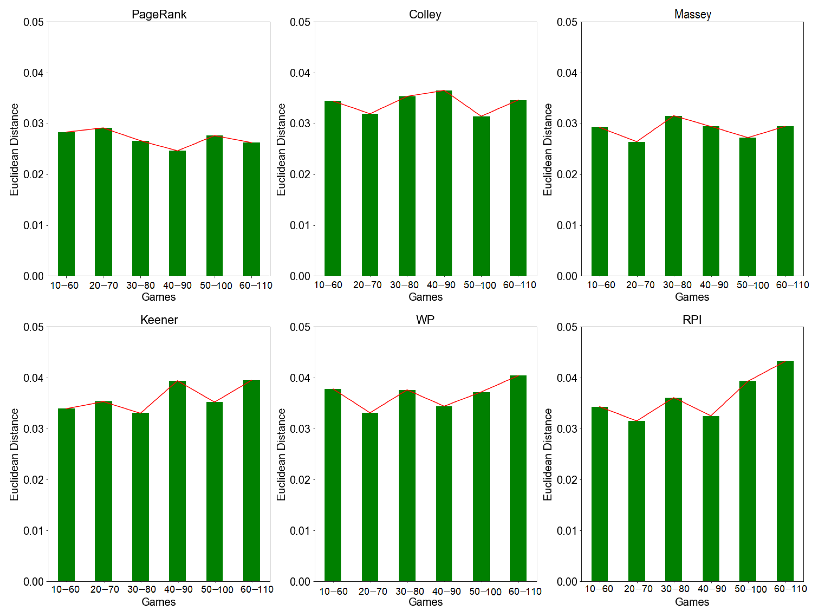
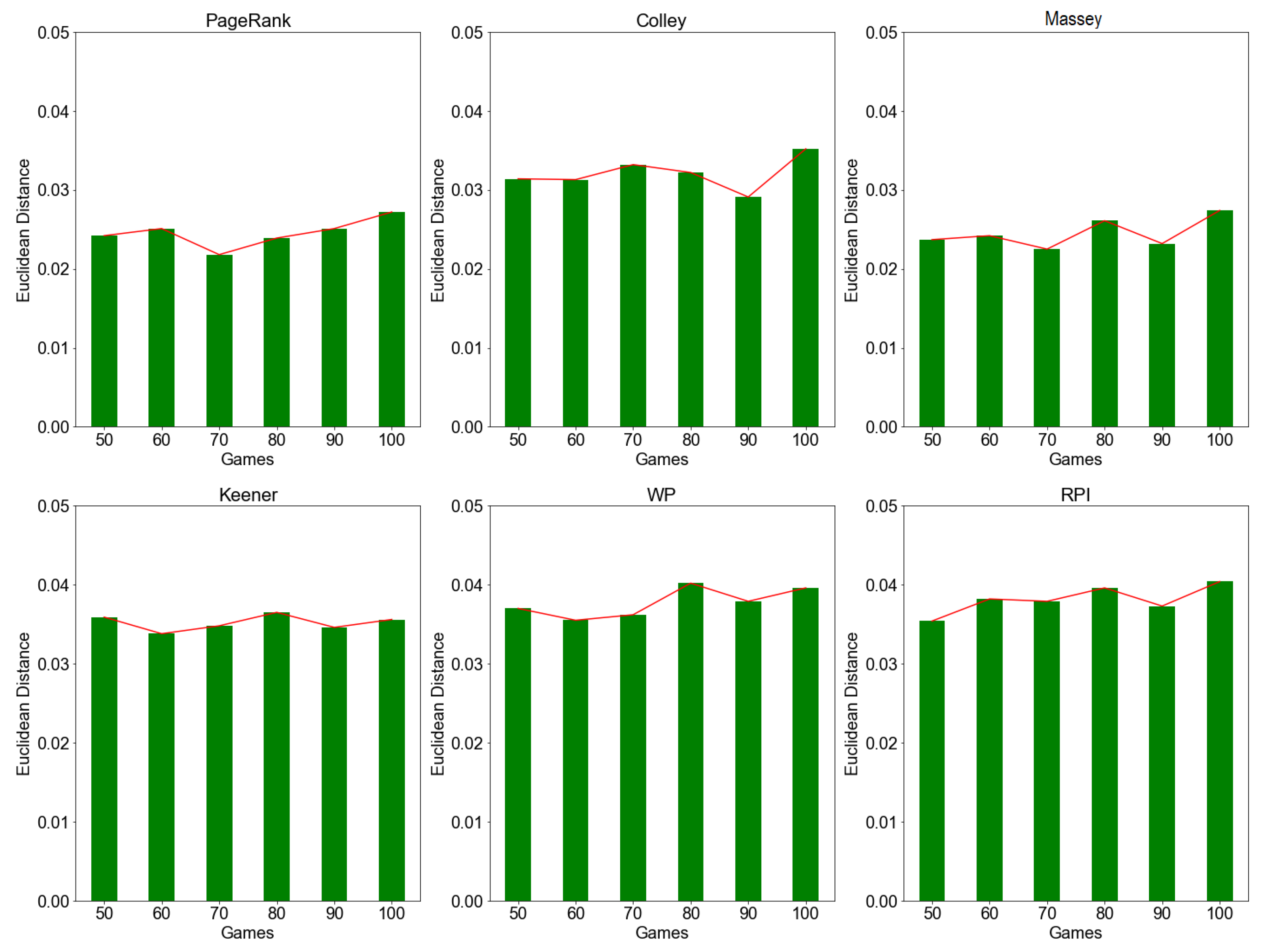
4.3. Rating Stability

We evaluate the rating stability based on the Euclidean distance measure described in Section 3.3. In this analysis, we compute Euclidean distance between two consecutive rating vectors obtained by rolling and expanding window approaches, respectively, to measure their similarity or deviation. In this scenario, the mean stability of the rating methods is based on average Euclidean distance $d_{RW}^2\left(t\right)$ and $d_{EW}^2\left(t\right)$ ($t=50,70,\dots$). In this case, we measure the mean distance between team rating vectors. The lower the $d^2\left(t\right)$ value, the more stable the rating method.

4.3.1. Evaluation by Rolling Window Approach

We measure the distance $d_{RW}^2\left(t\right)$ between two consecutive rating vectors. According to the results in Figure 1, for rolling window simulation, the distance values $d_{RW}^2\left(t\right)$ tend to change over time (i.e., on each window/game). Generally, PageRank and Massey recorded low average values of $d_{RW}^2=0.025$ and $d_{RW}^2=0.029$, respectively. On the other hand, Colley, Keener, WP, and RPI recorded higher distance values with an average of $d_{RW}^2\ge 0.035$. This implies those methods have lower rating stability due to high deviation (i.e., low similarity) in rating vectors.

4.3.2. Evaluation by Expanding Window Approach

We also compared and evaluated the rating stability of the investigated methods using the expanding window approach. Similarly, we measure distance $d_{EW}^2\left(t\right)$ between two consecutive rating vectors at incremental window size (i.e., after 50, 60, 70, …) as described in Section 3.3. The results in Figure 2 suggest that the distance values $d_{EW}^2\left(t\right)$ for expanding window simulation increase over time (i.e., on each window/game). Again, PageRank and Massey recorded low average distance values ranging between $d_{EW}^2=0.025$ and $d_{EW}^2=0.03$. Again, low $d_{EW}^2$ value implies low deviation (i.e., high similarity) in rating vectors and hence a high rating stability. Similarly, Colley, Keener, WP, and RPI recorded slightly higher average distance values ranging between $d_{EW}^2=0.035$ and $d_{EW}^2=0.040.$ This indicates that those methods have lower rating stability due to high deviation (i.e., low similarity) in rating vectors.

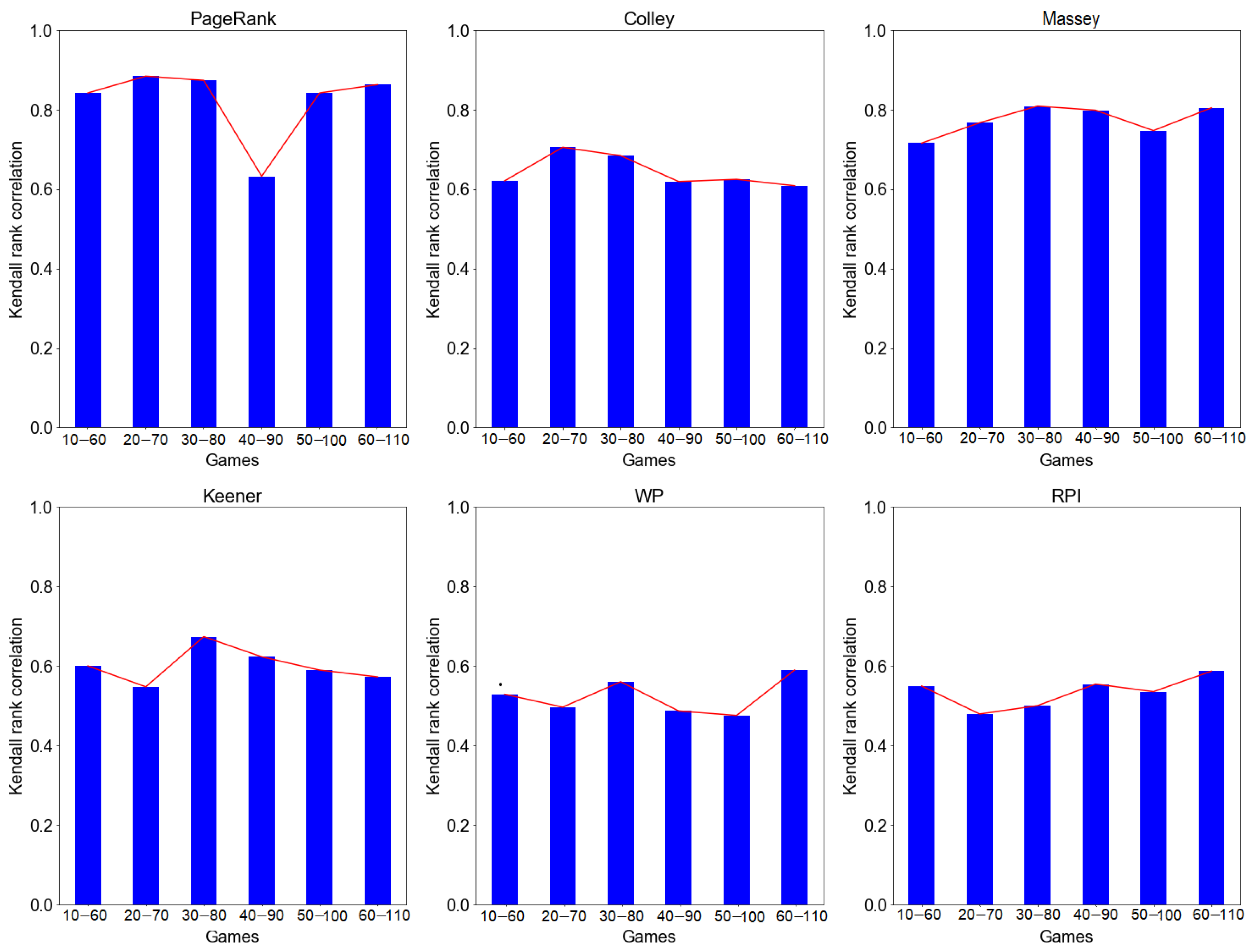
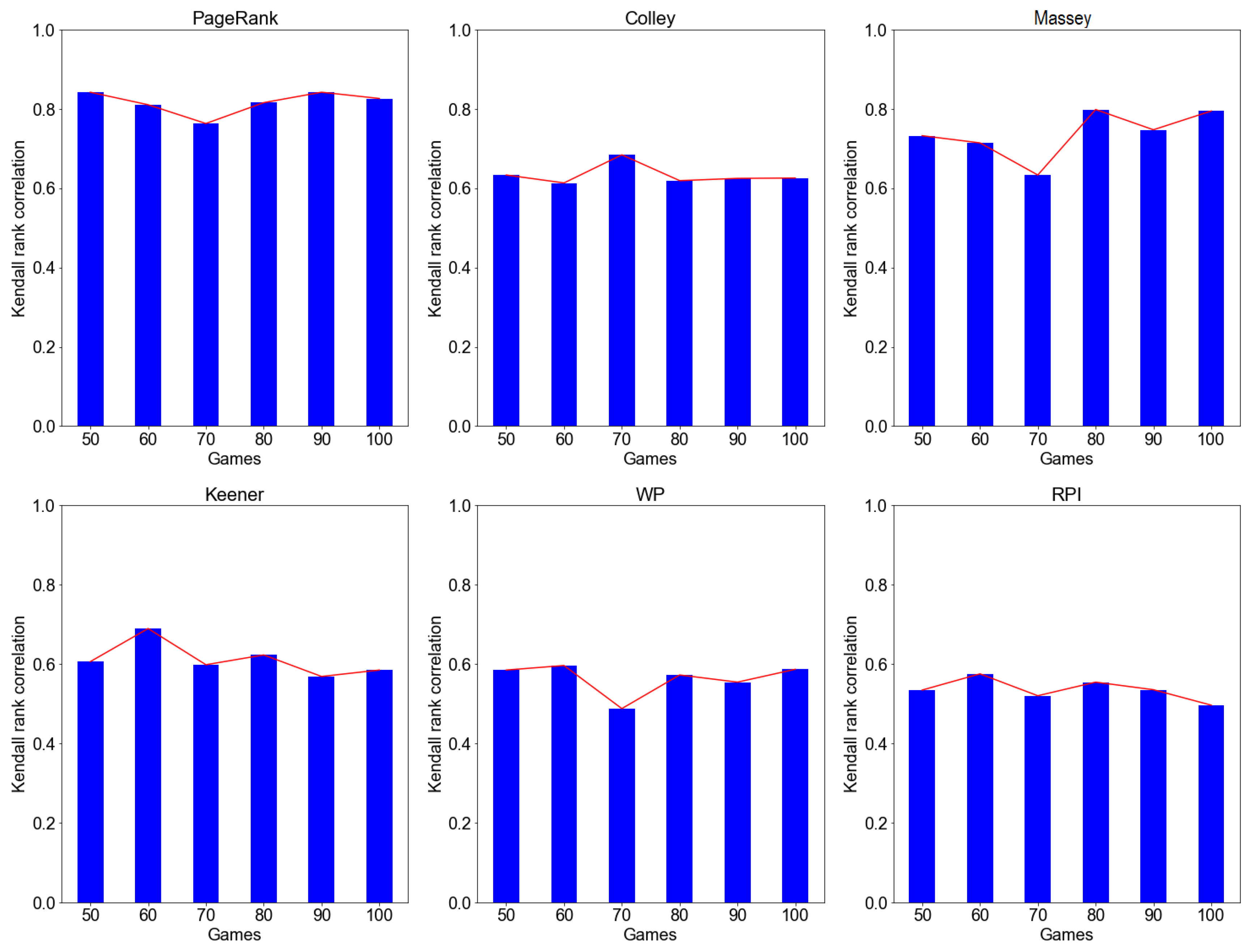
4.4. Ranking Stability

As mentioned in Section 3.4, we compared ranking stability for the investigated methods using rolling window and expanding window based on the Kendall tau method. Here, we consider rank correlation coefficient $\tau$ taking values between $-1$ and +1, which characterizes the degree of ranking stability (i.e., agreement between two rank lists). Statistically, $\tau$ measures the similarity (concordant and discordant) of two rank lists. The values of $\tau =+1$ indicate the highest possible ranking stability, i.e., the two rank lists are exactly the same, while $\tau =-1$ indicates low ranking stability, i.e., the two team rank lists are exactly the opposite, and $\tau \left(r\right)=0.00$ implies that one rank list is a random reordering of the other.

4.4.1. Evaluation by Rolling Window Approach

According the result in Figure 3, PageRank and Massey recorded the highest rank correlation, ${\tau }_{RW}\ge 0.60$ and ${\tau }_{RW}\ge 0.80$, respectively. On the other hand, both Colley and Keener recorded a rank correlation of ${\tau }_{RW}\approx 0.60$. However, WP and RPI recorded a low rank correlation, i.e., ${\tau }_{RW}\le 0.60$. In general, PageRank, Colley, and Massey have relatively stable ranking performance compared with Keener, WP, and RPI, which tend to be unstable over time (at different windows/number of games). ${\tau }_{RW}\le 0$ implies that all six investigated ranking methods show ranking stability using our rolling window approach.

4.4.2. Evaluation by Expanding Window Approach

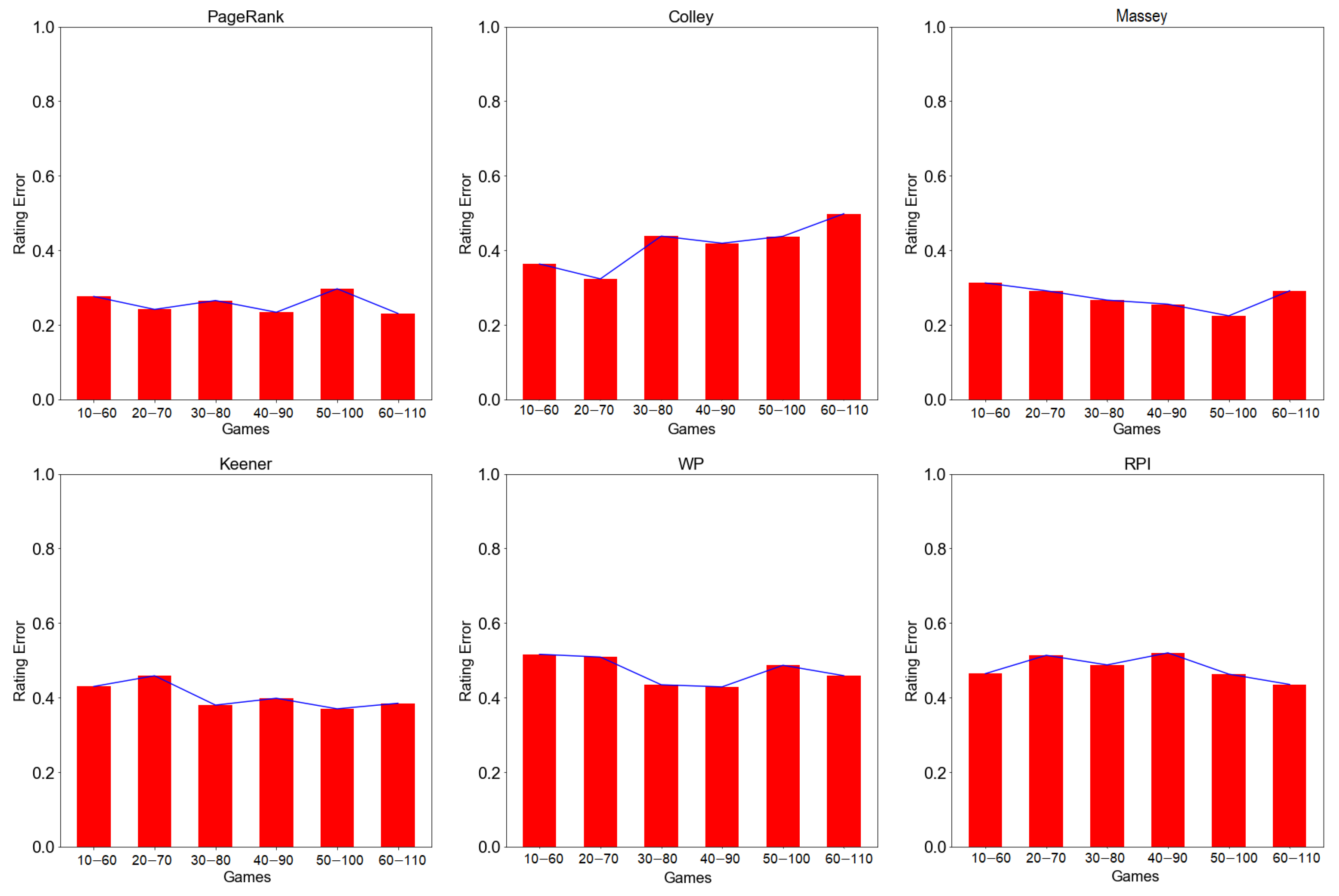
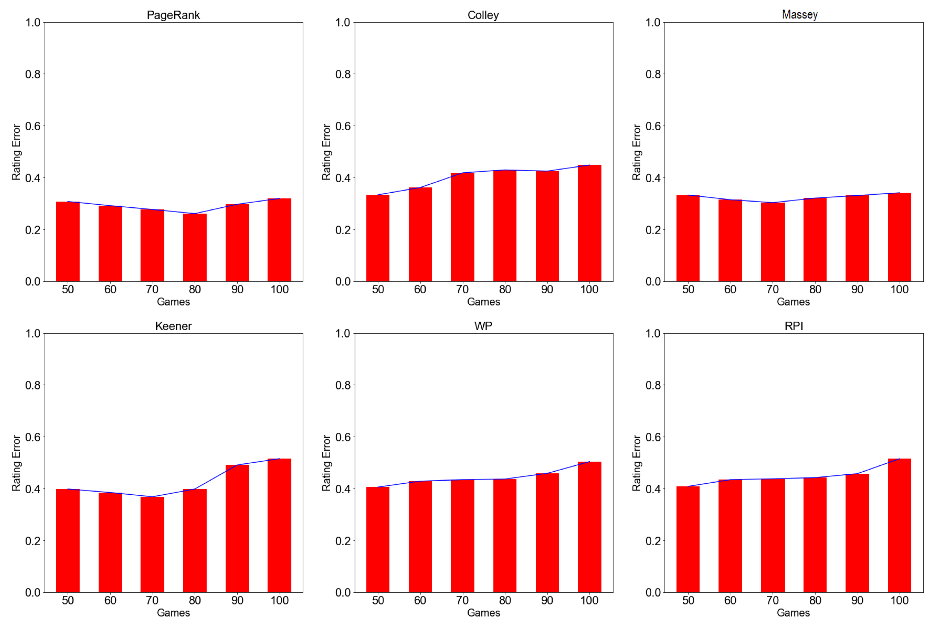
We further compared the ranking stability of all the investigated ranking methods using the expanding window approach. According to the result in Figure 4, PageRank, Colley, Massey, and Keener methods recorded a higher rank correlation value of ${\tau }_{EW}\le 0.60$ with PageRank recording highest values of ${\tau }_{EW}\ge 0.70$. WP and RPI recorded a relatively low rank correlation value of ${\tau }_{EW}\le 0.60$. Overall, the analysis indicates that as we increase/expand the window size (i.e., number of games), the rating stability tends to increase over time.

4.5. Rating Error

As described in Section 3.5, we evaluated the predictive power of the rating methods using a very simple and intuitive approach. For the training set, we considered a fixed number of games (50) or incremental number of games (50, 70, …) with respect to rolling window and expanding window simulations. For the test set, a fixed number of games (10 in our case), played right after the games considered in the training set, was used.

According to the evaluation results, the rating errors are shown in

Table 3. Average rating error for rolling and expanding window simulations.

	PageRank		Colley		Massey		Keener		WP		RPI
	RMSE	sd	RMSE	sd	RMSE	sd	RMSE	sd	RMSE	std	RMSE	sd
RW	0.2568	0.0188	0.4133	0.1156	0.2819	0.0318	0.4067	0.0435	0.4722	0.0927	0.4809	0.2220
EW	0.2826	0.0193	0.4025	0.0765	0.3237	0.0172	0.3859	0.0573	0.4446	0.0489	0.4425	0.0692

. It was evidenced that PageRank and Massey had a low average rating error, that is, $E_{\varphi }\&\le 0.2568$ and $E_{\varphi }\&\le 0.2819$, respectively. This leads to the hypothesis that both PageRank and Massey rankings had higher predictive power than the others. A more detailed comparison of rating error can be seen from Figure A1 and Figure A2 in Appendix B.

5. Discussions

To gain a deeper insight into how some widely used rating systems work, we compared the rating and ranking performance of six rating methods. We applied a forward-looking approach to compare and evaluate their ranking and rating stability. In our experimental investigations, we considered the 2014 English Primer League dataset for simulations (similar to NFL data used in a related study [12], or US major sports data used in [7]). Our approach provides an efficient tool to compare and evaluate the stability of ranking or rating of teams obtained by different methods.

We used a distance-based approach to compare the rating stability utilizing the Euclidean distance measure. It takes into consideration the difference of the consecutive rating vectors. Rating methods with small deviation measures tend to have higher rating stability [22,23]. According to the results in Figure 1 and Figure 2, PageRank generally recorded low deviation measures in both rolling window and expanding window simulation.

The results of the evaluation of ranking stability by rolling window and expanding window are presented in Section 4. Among the six methods we examined (PageRank, Colley, Massey, Keener, WP, and RPI), we observed the difference of ranking results at different time windows and window sizes using Kendall tau rank correlation. Some rating methods, such as WP and RPI rank are similar compared to the others. If we consider the round-robin tournament, the rank correlation coefficient changes irregularly over time at different window sizes.

We also conducted a comparison of rank–rate performance providing some new insights into the functionality of rating systems (see Table A1 and Table A2, Appendix A).

When we considered an increasing time window (by a constant factor), we observed that the Kendall tau rank correlation stabilized over time. This implies that the overall ranking is becomes generally more stable when approaching the end of the competition.

According to the prediction error results in Table 3, for the rolling window simulation, PageRank and Massey methods recorded a low mean prediction error of 0.257 and 0.282, respectively. On the other hand, WP (0.472) and RPI (0.481) recorded higher prediction errors. Further evaluation of the prediction error based on the expanding window approach shows a similar trend. However, PageRank and Massey recorded slightly higher prediction errors in this case, being 0.283 and 0.324, respectively. In contrast, Colley, Keener, WP, and RPI recorded slightly low prediction errors compared to the rolling window case. Colley, Keener, WP, and RPI tended to predict better using the expanding window approach (see Appendix B).

We have also seen that prediction error depends on the rating and ranking stability of the methods. Stable rating methods tend to record low prediction errors compared to less stable methods, in agreement with the findings in [24]. Generally, the findings of this study, in agreement with the related literature, suggest that PageRank is a more stable and robust rating method in the sport domain compared to the other five methods. PageRank, which was developed originally in the search engines domain [18], has been applied in various other domains as well as in sports. Just to mention some related studies, a time-dependent PageRank was also used for ranking sports tournaments [25,26]. PageRank was also applied on randomized sports data to rank teams and individual players in sports [27]. Our findings, in general, coincide with the previous ones showing the distinguished capability and performance of PageRank in rating and ranking compared to most of the other approaches.

6. Conclusions

This study presents a forward-looking approach to compare and evaluate six basic rating methods with two different simulation scenarios, namely a rolling window and an expanding window approach, respectively. Rank–rate comparison indicates that the PageRank and Massey methods are consistent and robust in rating and ranking teams in both rolling and expanding forward-looking approaches. Evaluation of ranking stability by using Kendall tau correlation coefficients shows that PageRank has a high rank correlation coefficient. This indicates its stability in ranking over time. Similarly, evaluation of rating stability by the Euclidean distance measure indicates both the PageRank and Massey methods have only a small change in distance measure in both simulation setups, hence showing a high rating stability in general. Evaluation of rating error suggests that PageRank has high predictive power in both rolling and expanding window simulations. In general, the PageRank and Massey methods performed well in both rolling and expanding window tests. Nevertheless, further comparisons may be needed to test their rating stability as well as their robustness in other applications.

References

1. Langville, A.N.; Meyer, C.D. Google’s PageRank and Beyond: The Science of Search Engine Rankings; Princeton University Press: Princeton, NJ, USA, 2011. [Google Scholar]
2. Rubinstein, A. Ranking the participants in a tournament. SIAM J. Appl. Math. 1980, 38, 108–111. [Google Scholar] [CrossRef]
3. Bouyssou, D.; Perny, P. Ranking methods for valued preference relations: A characterization of a method based on leaving and entering flows. Eur. J. Oper. Res. 1992, 61, 186–194. [Google Scholar] [CrossRef]
4. Chebotarev, P.Y.; Shamis, E. Characterizations of scoring methodsfor preference aggregation. Ann. Oper. Res. 1998, 80, 299–332. [Google Scholar] [CrossRef]
5. Vaziri, B.; Dabadghao, S.; Yih, Y.; Morin, T.L. Properties of sports ranking methods. J. Oper. Res. Soc. 2018, 69, 776–787. [Google Scholar] [CrossRef]
6. Constantinou, N.E.F.; Neil, M. Pi-football: A bayesian network model for forecasting association football match outcomes. Knowl.-Based Syst. 2012, 36, 322–339. [Google Scholar] [CrossRef]
7. Barrow, D.; Drayer, I.; Elliott, P.; Gaut, G.; Osting, B. Ranking rankings: An empirical comparison of the predictive power of sports ranking methods. J. Quant. Anal. Sport 2013, 9, 187–202. [Google Scholar] [CrossRef]
8. Chartier, T.P.; Kreutzer, E.; Langville, A.N.; Pedings, K.E. Sensitivity and stability of ranking vectors. SIAM J. Sci. Comput. 2011, 33, 1077–1102. [Google Scholar] [CrossRef]
9. Kardos, O.; London, A.; Vinkó, T. Stability of network centrality measures: A numerical study. Soc. Netw. Anal. Min. 2020, 10, 1–17. [Google Scholar] [CrossRef]
10. Segarra, S.; Ribeiro, A. Stability and continuity of centrality measures in weighted graphs. IEEE Trans. Signal Process. 2015, 64, 543–555. [Google Scholar] [CrossRef] [Green Version]
11. Costenbader, E.; Valente, T.W. The stability of centrality measures when networks are sampled. Soc. Netw. 2003, 25, 283–307. [Google Scholar] [CrossRef]
12. Langville, A.N.; Meyer, C.D. Who’s# 1?: The Science of Rating and Ranking; Princeton University Press: Princeton, NJ, USA, 2012. [Google Scholar]
13. Jiang, X.; Lim, L.H.; Yao, Y.; Ye, Y. Statistical ranking and combinatorial Hodge theory. Math. Program. 2011, 127, 203–244. [Google Scholar] [CrossRef] [Green Version]
14. Pickle, D.; Howard, B. Computer to Aid in Basketball Championship Selection. NCAA News. 1981, Volume 4. Available online: https://scholar.google.com/scholar?q=Pickle%2C+D.%3B+Howard%2C+B+Computer+to+aid+in+basketball+championship+selection.+NCAA+News%2C+1981%3B+Volume+4.&hl=en&as_sdt=0%2C5&as_ylo=&as_yhi= (accessed on 15 March 2022).
15. Massey, K. Statistical Models Applied to the Rating of Sports Teams. Unpublished. Bachelor’s Thesis, Bluefield College, Bluefield, VA, USA, 1997. [Google Scholar]
16. Colley, W. Colleyâs Bias Free College Football Ranking Method; Princeton University Princeton, NJ, USA. 2002. Available online: https://scholar.google.com/scholar?hl=en&as_sdt=0%2C5&q=Colley%2C+W.+Colley+%C3%A2s+Bias+Free+College+Football+Ranking+Method%3B+2002.&btnG= (accessed on 15 March 2022).
17. Keener, J.P. The Perron-Frobenius Theorem and the Ranking of Football Teams. SIAM Rev. 1993, 35, 80–93. [Google Scholar] [CrossRef]
18. Page, L.; Brin, S.; Motwani, R.; Winograd, T. The PageRank Citation Ranking: Bringing Order to the Web; Technical Report; Stanford InfoLab: Stanford, CA, USA, 1999. [Google Scholar]
19. Franceschet, M.; Bozzo, E. The Massey’s method for sport rating: A network science perspective. arXiv 2017, arXiv:1701.03363. [Google Scholar]
20. Liberti, L.; Lavor, C.; Maculan, N.; Mucherino, A. Euclidean distance geometry and applications. SIAM Rev. 2014, 56, 3–69. [Google Scholar] [CrossRef]
21. Kendall, M. A new measure of rank correlationâ? Biometrica 1938, 30, 81–93. [Google Scholar] [CrossRef]
22. HA, D. Ranking the players in a round robin tournament. Rev. Int. Stat. Inst. 1971, 39, 137–147. [Google Scholar]
23. Borodin, A.; Roberts, G.O.; Rosenthal, J.S.; Tsaparas, P. Link analysis ranking: Algorithms, theory, and experiments. ACM Trans. Internet Technol. 2005, 5, 231–297. [Google Scholar] [CrossRef]
24. Lasek, J.; Szlávik, Z.; Bhulai, S. The predictive power of ranking systems in association football. Int. J. Appl. Pattern Recognit. 2013, 1, 27–46. [Google Scholar] [CrossRef]
25. London, A.; Németh, J.; Németh, T. Time-dependent network algorithm for ranking in sports. Acta Cybern. 2014, 21, 495–506. [Google Scholar] [CrossRef] [Green Version]
26. Avron, H.; Horesh, L. Community Detection Using Time-Dependent Personalized Pagerank. In International Conference on Machine Learning; PMLR; 2015; pp. 1795–1803. Available online: https://scholar.google.com/scholar?hl=en&as_sdt=0%2C5&q=Avron%2C+H.%3B+Horesh%2C+L.+Community+detection+using+time-dependent+personalized+pagerank.+In+International+Conference+on+Machine+Learning%3B+PMLR%3A+2015%3B+pp.+1795%E2%80%931803&btnG= (accessed on 15 March 2022).
27. Zhou, Y.; Wang, R.; Zhang, Y.C.; Zeng, A.; Medo, M. Improving PageRank using sports results modeling. Knowl.-Based Syst. 2022, 2022, 108168. [Google Scholar] [CrossRef]
Figure 1. Rating stability based on Euclidean distance by rolling window approach. The figure above shows that the distance value d R W 2 t for PageRank, Colley, Massey, Keener, WP, and RPI methods changes over time at fixed window size (i.e., 10 games per window). Smaller value indicates a higher rating stability.
Information 13 00232 g001
Figure 2. Rating stability based on Euclidean distance by expanding window approach. The figure above shows that the distance value d E W 2 t for PageRank, Colley, Massey, Keener, WP, and RPI methods increases over time at incremental window size (i.e., an increase of 10 games per window). Smaller distance value indicate higher rating stability.
Information 13 00232 g002
Figure 3. Rank stability of PageRank, Colley, Massey, Keener, WP, and RPI methods using rolling window simulations.
Information 13 00232 g003
Figure 4. Rank stability of PageRank, Colley, Massey, Keener, WP, and RPI methods using expanding window simulations.
Information 13 00232 g004