Abstract
Software Product Line (SPL) developments include Variability Management (VA) as a core activity aiming at minimizing the inherent complexity in commonality and variability manipulation. Particularly, the (automated) analysis of variability models refers to the activities, methods and techniques involved in the definition, design, and instantiation of variabilities modeled during SPL development. Steps of this analysis are defined as a variability analysis process (VA process), which is focused on assisting variability model designers in avoiding anomalies and/or inconsistencies, and minimizing problems when products are implemented and derived. Previously, we have proposed an approach for analyzing variability models through a well-defined VA process (named SeVaTax). This process includes a comprehensive set of scenarios, which allows a designer to detect (and even correct in some cases) different incompatibilities. In this work, we extend SeVaTax by classifying the scenarios according to their dependencies, and by assessing the use of these scenarios. This assessment introduces two experiments to evaluate accuracy and coverage. The former addresses responses when variability models are analyzed, and the latter the completeness of our process with respect to other proposals. Findings show that a more extensive set of scenarios might improve the possibilities of current practices in variability analysis.
1. Introduction
The variability management area involves a set of methods and techniques aimed at providing flexibility within a Software Product Line (SPL) development and supporting, at the same time, mechanisms for defining, designing, implementing and testing variabilities. In addition, since variability is defined at early stages in the software development, promoting special management mechanisms during the whole life cycle is really important.
Within this area, the (automated) analysis of variability model research field has emerged, focusing on a set of techniques, activities and/or methods for verifying the consistency and correctness of the variability models and their configurations towards a consistent product generation. This field, which is also named the (automatic) verification of product line models [1,2], has attracted special attention from the SPL community, resulting in an extensive number of approaches with different mechanisms for improving the analysis.
Although there is no consensus about the activities included in the (automated) analysis of variability models [3], the research community agrees on a set of base activities included in the variability analysis process (VA process), as shown in Figure 1.
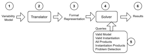
Figure 1.
General Process for Automated Analysis of Variability Models.
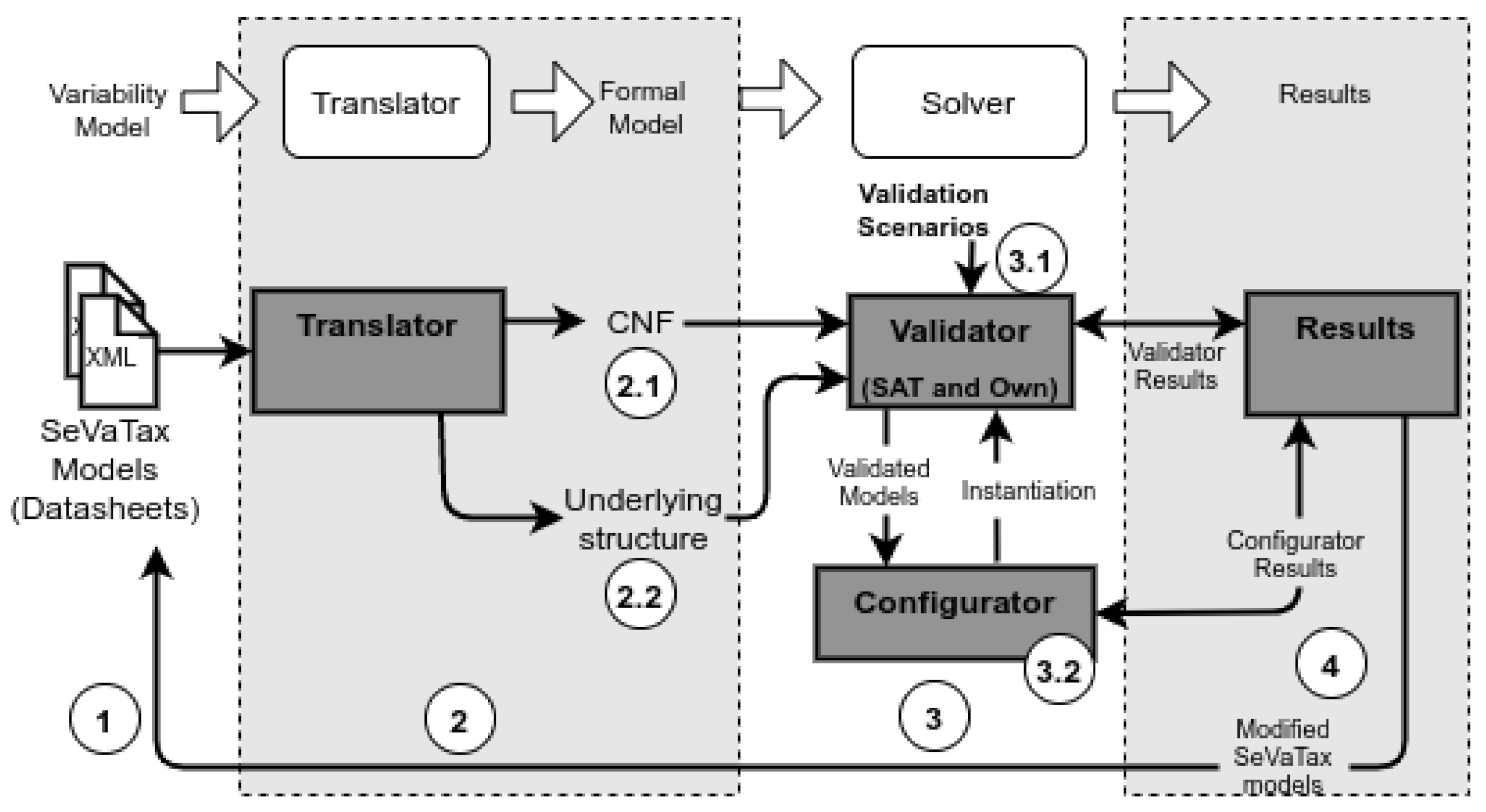
The main input (component 1 in the figure) consists of one (or many) variability models, depending on the variability modeling approach is being used. Following, the translator activity (component 2) is responsible for translating the model into a formal representation (component 3), which represents variabilities in logical terms. Then, a solver (component 4) is responsible for validating the formal model, after receiving a set of validation scenarios or queries (component 5) that the solver is capable of answering. The outputs of this activity are the results (sixth component) of the analysis process. These results can be identifications of anomalies and/or redundancies in the variability models, and sometimes new corrected models.
Current proposals in the literature define different mechanisms for implementing each component of the VA process. For example, the inputs of the process are modeled by using Feature Models (FM) [4], Orthogonal Variability Models (OVM) [5], Common Variability Languages (CVL) [6], and so on. At the same time, the translator and the formal representation may be different resulting in models depicted as Constraint Satisfaction Problem (CSP), Conjunctive Normal Form (CNF), Description Logic (DL), and so forth. Therefore, the set of proposed solvers depends on the formal representation is being applied; for example, CNF models are validated with SAT solvers such as Sat4j (www.sat4j.org/), or Choco (www.choco-solver.org), meanwhile DL models are validated with ontology reasoners such as RACER (https://franz.com/agraph/racer/) or FACT++ (http://owl.man.ac.uk/factplusplus/). However, although there are different mechanisms proposed, there are still open issues and challenges that have not been addressed [7]; for instance, a wider support for identifying and correcting variability errors, further studies about different quality attributes (QA) and the development of standard benchmarks for their analysis, the definition of minimal standard operations (queries) that solvers should respond to, and so forth.
Considering this context, in this work, we extend previous works proposing the SeVaTax process in order to automatically support the activities and provide solutions about open research issues.
This paper is organized as follows. The next section analyzes related works focused on the VA process. Section 4 describes our SeVaTax process showing specific activities, as well as the extended scenarios. In Section 5, we provide two experiments for evaluating accuracy and coverage. Conclusions and future works are discussed afterwards.
2. Previous Work and New Contributions
In order to clarify the contributions of this paper, first we introduce the scope of our previous work as follows:
- In Reference [8], we presented the first version of the SeVaTax process. The main aspects of this version were the SeVaTax model based on collaborative diagrams of UML with annotated variability (in OVM notation), a formalization in CNF, and the definition of 17 validation scenarios considering mismatches and/or anomalies on SeVaTax models. The use of these scenarios allowed to define the set of feasible inconsistencies, anomalies and redundancies present in the variability models, for which solvers provided a response, such as identification, explanation, or even correction when it was possible. In addition, we performed an evaluation by comparing our SeVaTax analysis process against two other approaches in the literature;
- In Reference [9], we presented an extension of the SeVaTax model, named scope operators, in order to include inter-related variability relations together with a proposal for verification (through the definition of more specific validation scenarios). In addition, we performed an evaluation of the impact of these extensions in the performance of our supporting tool;
- In Reference [7], we presented a systematic literature review on analysis of variability models. Specifically, we defined a classification framework, which considers the main activities involved in the (automated) analysis of variability models (Figure 1). The framework was applied to 43 primary studies, drawing strengths and challenges as well as research opportunities.
Other published works, less related to the VA process but analyzing changes in some parts or abstracting the process itself, were presented in [10,11]. In Reference [10], we proposed a formalization of SeVaTax models expressed in first order logic, and introduced a encoding allowing extended reasoning capabilities. The formalism was verified by analyzing consistency and dead services. In Reference [11], we proposed a framework for the VA process in order to combine automatic variability analysis tools, which can be adapted to specific requirements of a variability management case.
Considering these previous works, here we extended the SevaTax process capabilities in order to face with some challenges and open issues defined in the literature (widely described in the related work section) [7]. Specifically, we are interested in four of these challenges. They are:
- Challenge 1: Define the set of basic operations (queries) that the VA process must support. This challenge is related to the queries/validation scenarios that a VA process must be able to understand together with the type of responses generated. Here, we extend the query component of Figure 1 by adding more than ten validation scenarios generating a more comprehensive set of variability evaluation and identification possibilities;
- Challenge 2: Include extended variability primitives together with their specific operations. This challenge proposes the extension of semantic representations in the variability models to describe particularities of specific domains. The extension of variability model representations was previously presented in [9] specifically with the addition of scope operators. However, in this work we focus on the validation of these operators through the definition of new validation scenarios together with correction capabilities;
- Challenge 3: Add more support for error correction. This challenge is related to challenge 1 with respect to the results provided by the proposals. There is a need of more assistance in error correction. Particularly, the specification of more specific validation scenarios provides us with the possibility of identifying the services in the SeVaTax model generating incompatibilities. Thus, we can provide better correction mechanisms;
- Challenge 4: Add more rigorous evaluations. This challenge highlights the need of more rigorous evaluations of the VA process in order to measure quality attributes, such as performance, usability, accuracy, completeness, and so forth. Some of these evaluations have been performed also in the previous works. For example, performance in [9] and a preliminary comparison of completeness in [8]. Here, we extend the evaluations for analyzing accuracy and coverage of the SeVaTax process.
3. Related Work
The variability management area has been widely researched during recent years. This can be seen in the wide number of secondary studies addressing proposals, which implement one or more variability management tasks. In Reference [7] we analyzed twelve secondary studies, considering five of them particularly related to the VA process [3,12,13,14]. For example, in [13], a systematic review of domain analysis tools analyzes validation functionalities such as support for documentation, links between features and requirements, and the existence of support for consistency checking. In Reference [3] we found a wide review of fifty-three proposals, which analyzes activities included in the VA process, but applied to feature models only. Here, the authors define a classification of thirty feature analysis operations and apply them to the proposals. Then, in Reference [14] the authors present a comparison of automated analysis using Alloy [15] for feature models (FM). They analyze the support of nine proposals over ten feature analysis operations. Finally, in Reference [12], the authors analyze ten Textual Variability Modeling Languages (TVML) in order to show capabilities of these languages according to modeling, derivation and verification activities.
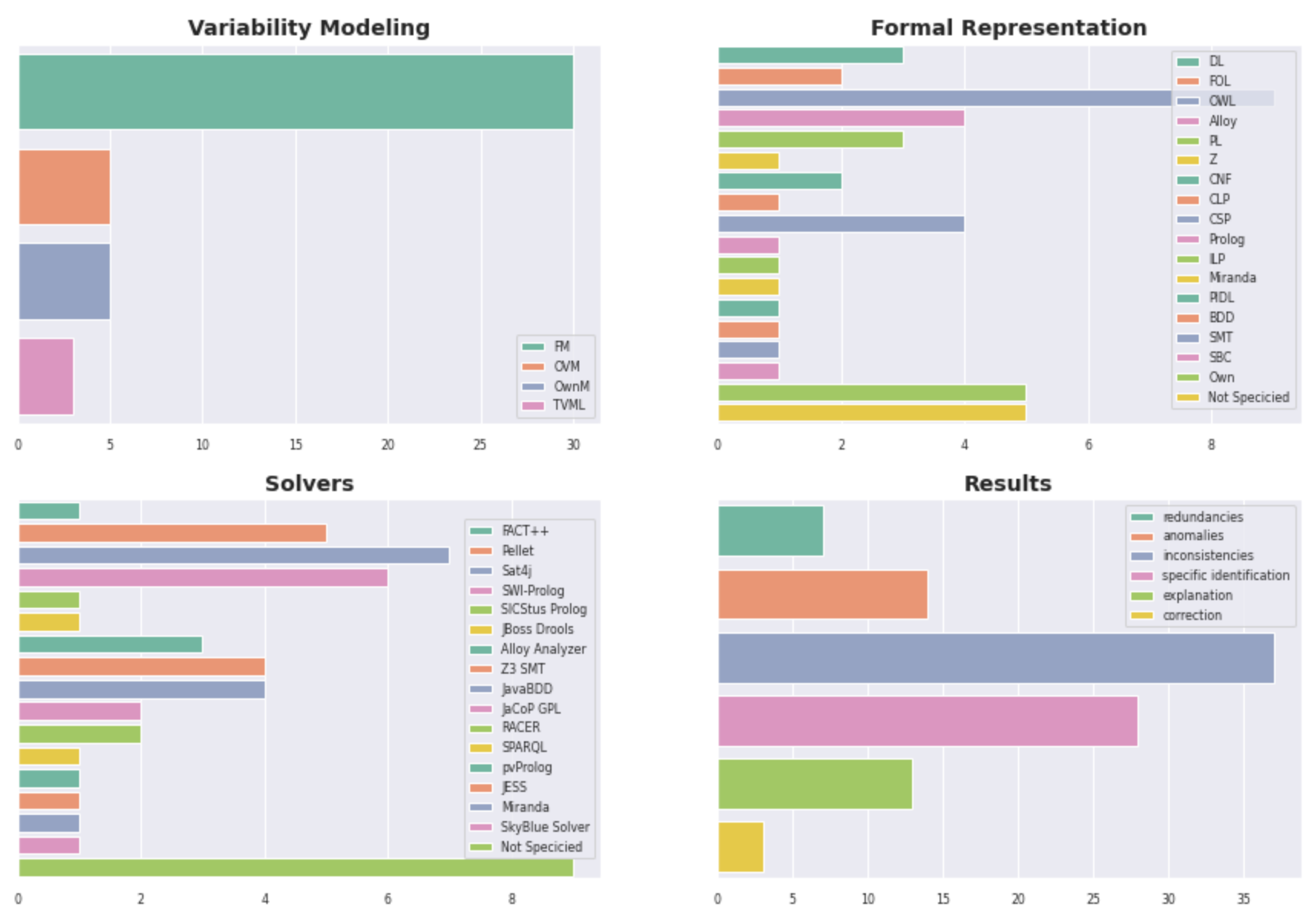
All these secondary studies, including ours, denote the wide range of different approaches and techniques used in the VA process. In particular, in [7] we have analyzed forty-three primary studies published during 2007–2018, addressing the way each primary study implements each activity of the VA process. A summary of the different approaches and techniques can be seen in Figure 2.
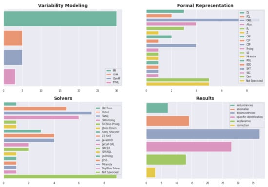
Figure 2.
Number of different approaches addressing each component of the VA Process.
For example, in the Variability Modeling bar-chart we can see that Feature Model (FM) [4] is the approach most commonly used (72%, that is, thirty primary studies). Fall into this category proposals such as FAMA-FM [16], FeatureIDE [17], SPLOT [18], and so forth. Then, 22% (five proposals) use OVM [5] or own model (OwnM) approaches. Examples are Braun et al. [10] and FAMA-OWM [19] for OVM approaches; and COVAMOF-VS [20] and DOPLER [21] for own models. Finally, the TVML approach is used by only three proposals [22]. At the same time, some studies allow more than only one modeling approach, such as Variamos [1] and Metzger et al. [23].
In the Formal Representation bar-chart we can see more than fifteen formal languages used in the different primary studies analyzed. The logic representation most commonly applied is OWL [24] (nine proposals). Falls into this category proposals such as Rincon et al. [25] and Langermeier et al. [26].
Following, in the Solvers bar-chart we can also see a wide number of different solvers applied. We observe that Sat4j is the most frequently used; meanwhile other solvers, such as ontological reasoners (RACER, FACT++, SPARQL (https://www.w3.org/TR/rdf-sparql-query/) and Pellet (http://pellet.owldl.com/)) are also applied by several studies such as Afriyanti et al. [27] and Wang et al. (2007) [2].
Finally, according to the VA process, we must consider queries the solver is capable of answering and the provided results. In this case, in [7], we considered both aspects together by analyzing whether proposals can identify incompatibilities in the variability models (according to the classification proposed in [28]). Thus, in the Results bar-chart of Figure 2, we can see the following items analyzed:
- Redundancy: proposals can identify whether the same semantic information is modelled redundantly in multiple ways;
- Anomaly: proposals can detect whether some required configurations of variability models are never possible but they should be. Examples of anomalies are the well-known problems analyzed as dead features, conditional dead features, false optional, wrong cardinalities, and so forth [3];
- Inconsistency: proposals can found contradictions represented in the variability models. In general, this happens when the variability models cannot be ever instantiated. For instance, the inconsistency called void feature model includes models that cannot derive any product;
- Specific identification: proposals can identify specific dependencies or features causing some of the previous problems;
- Explanation: once identified, proposals provide a textual explanation about the problem found;
- Correction: proposals can perform an automatic correction or provide suggestions about the corrections needed.
The most supported response is the detection of inconsistencies in the variability models (with more than thirty proposals); while the lesser one is the correction of models, with proposals such as FD-Checker [29] and Wang et al. (2014) [30].
As the conclusions of this secondary study, in [7] we have defined eight specific challenges or open issues that must be considered in future research. Specifically, in this work we address four of them, as we described in Section 2.
In addition, we can cite other more recent related works, such as [31,32,33]. For example in [31] authors define restrictions on the use of SysML (https://sysml.org/) for annotated product line models. These constraints are then used for checking dead and false optional features. In [32], the authors propose the use of Monte Carlo tree search [34] for feature model analyses. The activities performed are related to feature selection during product derivation, also analyzing the performance of the selection. The framework proposed allows to find an empty configuration, an empty feature model, and also valid configurations proposing one of them as the best one. Finally, in [33] authors present a research tool for model checking variability. The tool uses a labeled transition system with variability constraints in order to analyze and configure feature models. In particular, the tool allows to analyze and correct ambiguities, remove false optional and dead services by interacting with nodes and edges of the transition model.
Although all these related works propose novel ways for representing variability models and improving the analyses and configurations, none of them provide new capabilities for incompatibility detection (component 5 of Figure 1).
4. Materials and Methods
The SeVaTax process is composed of four modules with their input/output flows. Figure 3 shows those modules, according to the general analysis process defined in Figure 1. Let us further describe each component of Figure 3 in the next subsections.

Figure 3.
SeVaTax analysis process.
4.1. SeVaTax Models (Component 1)
The SeVaTax model emerges as a design model defined for an SPL methodology applied to several geographic subdomains. In previous works [35,36] we defined this model based on a functionality-oriented design. That is, each functionality of the SPL is documented by a functional datasheet representing the set of services, commons (Common services are services that will be part of every product derived from the SPL) and variants, which interact to reach the desired functionality.
Each datasheet is documented by using a template composed of six items containing an identification, such as a number or code; a textual name, describing the main function; the domain in which this functionality is included; the list of services required for fulfilling this functionality; a graphical notation, which is a set of graphical artifacts showing the service interactions (as common and variant services); and a JSON (https://www.json.org/json-es.html) file specifying the services and their interactions. Within the graphical notation item (of the datasheets) any graphical artifact might be used; and particularly, we use an artifact based on variability annotation of collaboration diagrams (of UML). The required variability, according to the functionality to be represented, is attached to the diagrams by using the OVM notation [5].
The complete set of interactions in our variability models is specified in Table 1. As we can see, they are divided into variability types, for denoting the variant interactions among services; dependencies, for denoting interactions between services; and scope, for specifying the scope of each variant point. SeVaTax models introduce three novel interactions: the use dependency and two scope operators. The former specifies a dependence between common services, which are not necessarily associated with a variation point; meanwhile the latter are related to the scope defined for a variation point when it must be instantiated [37]. There are two possibilities here: (1) a Global Variation Point (GVP) specifies that, if the variation point is instantiated in a specific way, it will be applied in that way for all functionality, including that variation point; and (2) a Specific Variation Point (SVP) specifies that the instantiation of the variation point is particular for each functionality, including that variation point.

Table 1.
Interactions defined for modeling SeVaTax models.
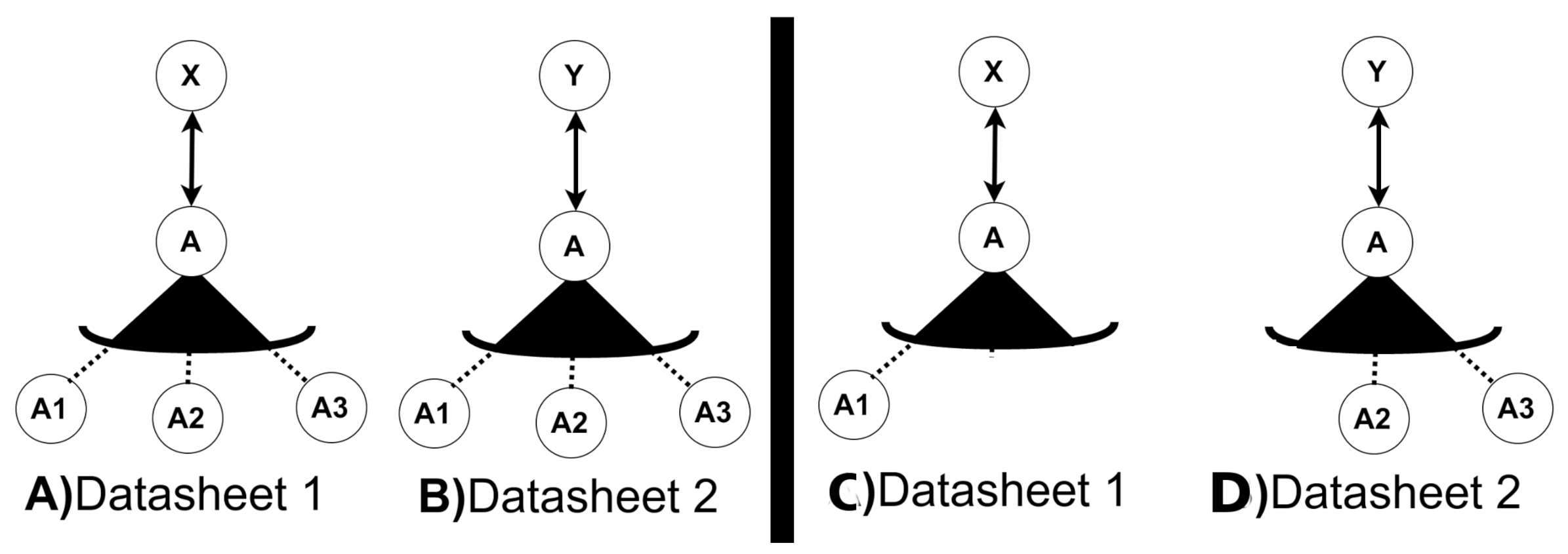
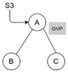
The scope operators have been added to the SeVaTax models [9] in order to design functionalities with the possibility of reusing variation points and their instantiations. As an example for clarifying these operators, we can see Figure 4A,B containing a Variant Variation Point, named A, with three variants (, and ) and two different services (X and Y) in different variability models of two datasheets (1 and 2 respectively). Considering the two scope operators, we have the following two possibilities:
- GVP operator: if a is attached to the variation point A in both models, there will be an only one possibility to instantiate it. That is, it will be valid to have instantiations such as Figure 4C or D but not both of them. Only one instantiation will be valid for the whole SPL platform for A;

Figure 4.
An example of the use of scope operators in two datasheets.
Figure 4.
An example of the use of scope operators in two datasheets.
In previous works, we have modeled SeVaTax models and their datasheets for two geographical subdomains—marine ecology [35,36] and paleontology [38]. As an example, Table 2 shows a variability model for the Add New Excavations datasheet (paleontology subdomain).
Table 2.
An example of the functional datasheet for Add New Excavations (extracted from [38]).
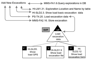
For example, in the SPL of the paleontology subdomain [38], we can reuse the same variation point in two functionalities. One of them is Add New Excavations (showed in Table 2), and the other one is Add New Paleontologist, showed in Figure 5. As this last functionality lets the user to add a new excavation for indicating the excavation in which he/she was involved, the variation point Load excavation data is reused in the same way for both functionalities (Here, only a part of the Add New Excavations is reused, specifically the service PS-T4.20). The variation point is also defined as because it can be instantiated, in a different way, for each of those functionalities.
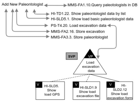
Figure 5.
SeVaTax Model for Add New Paleontologist functionality.
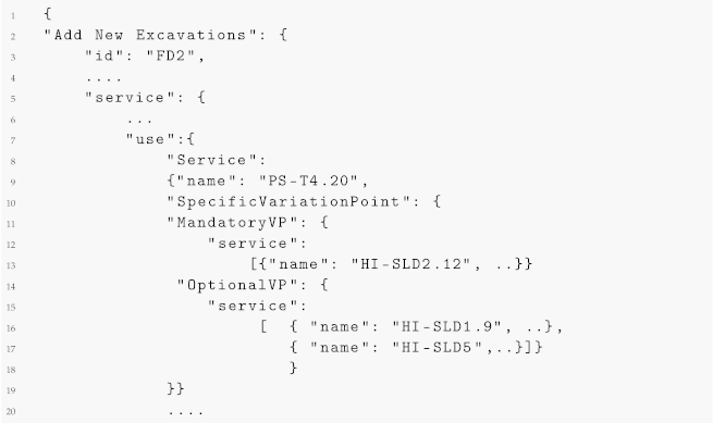
Finally, the last item of the datasheet is a JSON file built according to the JSON properties (showed in the second column of Table 1). This file is generated to allow automatic processing of SeVaTax models.
In Listing 1 we can see the JSON file for the SeVaTax model shown in Table 2 for the variation point.
Listing 1.
Part of the JSON file for representing the SeVaTax model shown in Table 2.
Listing 1.
Part of the JSON file for representing the SeVaTax model shown in Table 2.
 |
4.2. Translator (Component 2)
The translator is responsible for parsing the JSON files (from the datasheets) and generating two outputs, a formal representation in CNF (Component 2.1 of Figure 3) and an instantiation of the underlying structures (Component 2.2 of Figure 3). The CNF representation was presented in [8,9] for each interaction defined in Table 1. As an example of the translation activity, in Table 3 we show examples of parts of SeVaTax models together with the logic model, CNF translation, and the numeric representation of the CNF. This last column represents the inputs for the solver in the next activity.
Table 3.
Translation of parts of SeVaTax models.
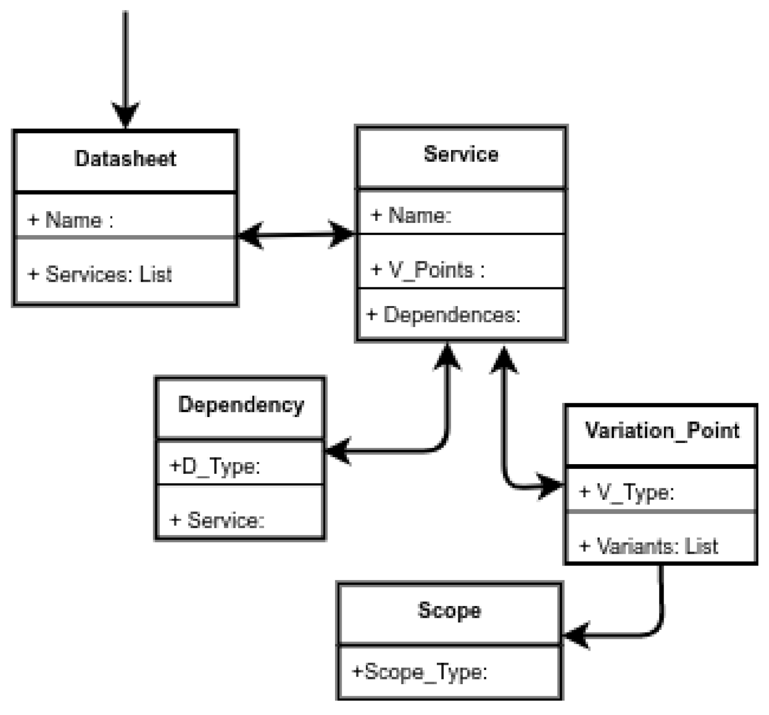
For supporting the validation activities, we defined underlying structures that instantiate each service and interaction of each variability model. These underlying structures have been restructured from previous work [9] in order to improve the way scenarios are detected and identified. In Figure 6 we can see the metamodel for representing each variability model of the datasheets. To represent the variation points, we register the variation point scope (which is unique) together with the variation point list. Each variation point contains a variability type and a variant list, where each variant corresponds to a service. Then, as each service belongs to one or more variability models (of each involved datasheet), it is possible to represent cross-dependencies and analyze the scopes of the variation points.

Figure 6.
Metamodel for representing underlying structures.
4.3. Validator (Component 3.1) and Results (Component 4)
The validator is responsible for identifying possible problems in the variability models when developing an SPL. Generally, the design of variability models is an error-prone task, that is, the development of an SPL involves functionalities and their associated variability models, which can show a conflict among functionalities. For example, in [38], we applied SeVaTax models (represented as functional datasheets) for designing functionalities in the paleontology subdomain; however, these functionalities could have contained incompatibilities that must be analyzed in order to avoid problems during implementation and/or product derivation. To illustrate this, in Figure 7 we introduce an anomaly as a require dependency in the variability model showed in Table 2—a mandatory service (HI-SLD2.12) requires an optional one (HI-SLD1.9), making it also present in all products. This is an example of the kind of problems that the validator must detect.
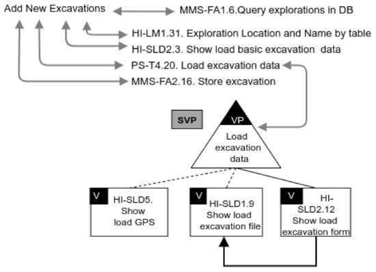
Figure 7.
Variability model for Add New Excavations with an anomaly.
Possible problems of the variability models are seen as queries that solvers are capable of answering. In this way, before configuring a solver, it is important to define the specific queries supported by the analysis process, that is, the set of questions that solvers are capable of answering. In previous works [8,9,10], we have defined a set of questions classified as validation scenarios. They represent possible problems of the variability models to be analyzed for providing more specific responses.
In the related work section (Section 3), we showed the most common responses provided by proposals in the literature. They were classified as results, indicating the support for incompatibilities (redundancies, anomalies and inconsistencies) and the level of detection, that is, from a simple identification to a correction of the specific problem. These incompatibilities have been classified in the literature as independent problems, that is, not associated to specific domains. In our work we also define them as generic or independent, which means they can be found in different variability models of different domains, but always representing classified incompatibilities.
After analyzing our previous works and the most common responses in the literature, here we extend and reorganize our previous validation scenarios in order to consider incompatibilities with respect to two main parameters: (1) the variability interactions used in the models; and (2) the severity of the incompatibilities (according to the proposal by Massen & Lichter [28]).
For the first parameter, as we have showed in Table 1, the interactions are divided into (1) variability types, for denoting mandatory, optional, alternative and variant variation points; (2) dependencies, for the use of uses, requires, and excludes restrictions among services; and (3) scope, for specifying the scope of each variation point at the moment of being instantiated. In this way, the variability models are firstly classified into validation scenarios by considering incompatibilities among the variability interactions involved.
Considering the second parameter, the variability models are also classified to explicitly incorporate the severity of an incompatibility. Thus, a variability model can present redundancies, when the model includes the same semantic restriction at least twice; anomalies, when the model is representing something irregular (According to Massen & Lichter an anomaly exists when potential configurations would be lost, though these configurations should be possible) that requires special attention; and inconsistencies, when the model presents contradictions making the analysis and derivations (in instantiated products) impossible. Obviously, the last one represents the most severe problem.
This new classification into the two parameters generates a comprehensive suite of validation scenarios defining possible incompatibility patterns among services. At the same time, the severity of an incompatibility helps on the identification and reparation actions when these patterns are found. In this way, from our classification of validation scenarios, we can specify specific responses provided by our validator, and take the required actions.
For each scenario, responses might be:
- Warning (W)
 : an alert is generated describing a possible problem together with the involved services;
 - General Identification (GI)
 : the services generating the conflict are identified, but it is not possible to identify a specific scenario;
 - Specific Identification (SI)
 : the scenario generating the conflict is identified. The causes of this conflict and the services involved for assisting the solution should be identified;
 - Repair (R)
 : the scenario that generates the conflict is identified and a pre-established solution is applied/suggested. The required action can be modification or elimination.
These validators’ responses are obtained by using the SAT solver (Sat4j) and/or the underlying structures to identify and correct the incompatibility, whenever it is possible. In general, the underlying structures are used as a support when the SAT solver is not enough to specifically identify the services generating the incompatibility. Similarly, for the repair response, the underlying structures are essential for suggesting the actions that could be carried out. To understand the use of these structures, in Figure 8 we show part of the instantiation of the variability model for the Add New Excavations functionality of Figure 7. Specifically, we represent the variation point PS-T4.20 with one mandatory and two optional services. We can also see the requires dependency representing that HI-SLD2.12 requires the HI-SLD1.9 service. In this case, when the anomaly is detected, the instantiation is used to identify the specific services involved and provide a solution.
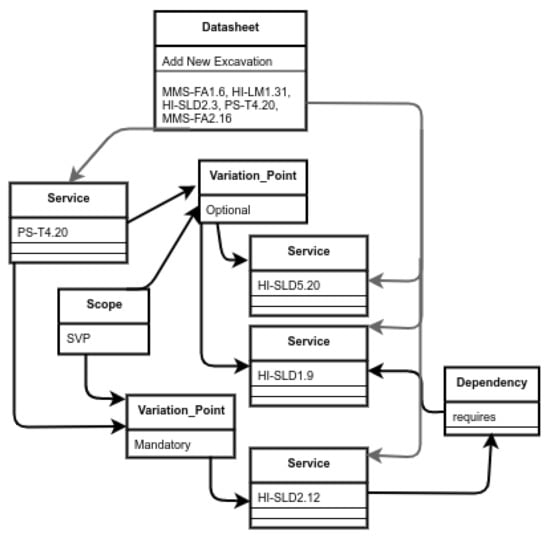
Figure 8.
Part of the instantiation of Add New Excavations functionality of Figure 7.
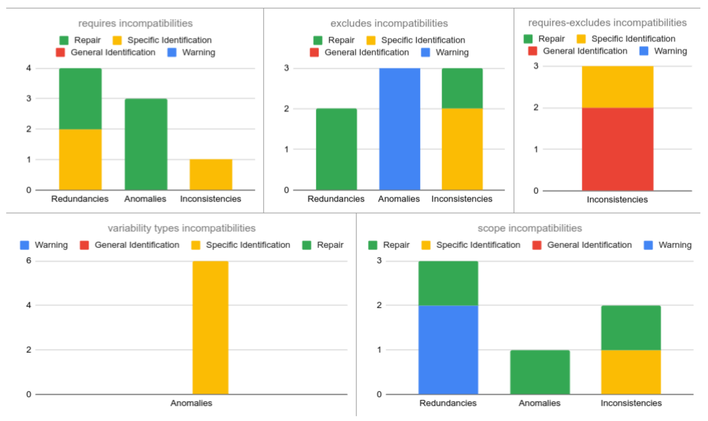
In Figure 9, we can see the classification of validation scenarios considering the use of the requires dependency. Columns are labeled according to the three different types of severity; meanwhile the rows represent the type of variability. For instance, a service with a requires dependency presents anomalies when the dependency is directed towards another optional, variant or alternative service, making it present on every instantiated product. An inconsistency appears when a requires dependency is directed towards another alternative service from the same variation point, that is, the variability model cannot be ever instantiated. Finally, in the figure we can see also variability models with redundancies, as the last ones. These scenarios, are independent from the variability types involved and they are present when a requires dependency is directed towards a parent, the same service, or a set of services transitively.
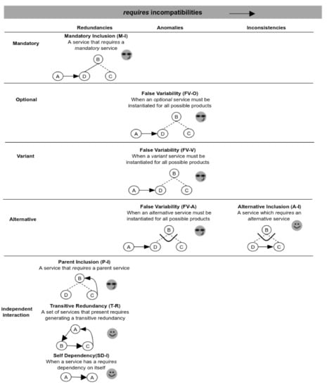
Figure 9.
Validation scenarios involving requires incompatibilities.
Figure 9 also shows the responses provided by our validator to each validation scenario defined. In five of them, our validator suggests correcting the incompatibility and in the rest ones, it provides a specific identification of the incompatibility and the involved services. For example, for the anomaly of the FV-O scenario (in the figure), each configurable service is evaluated individually by the SAT solver. To do so, it is necessary to pre-setup the service as false and the variation point (containing this service) as true in the CNF. If the generated CNF is inconsistent, then the service is a false optional.
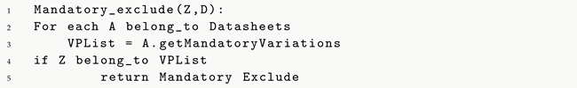
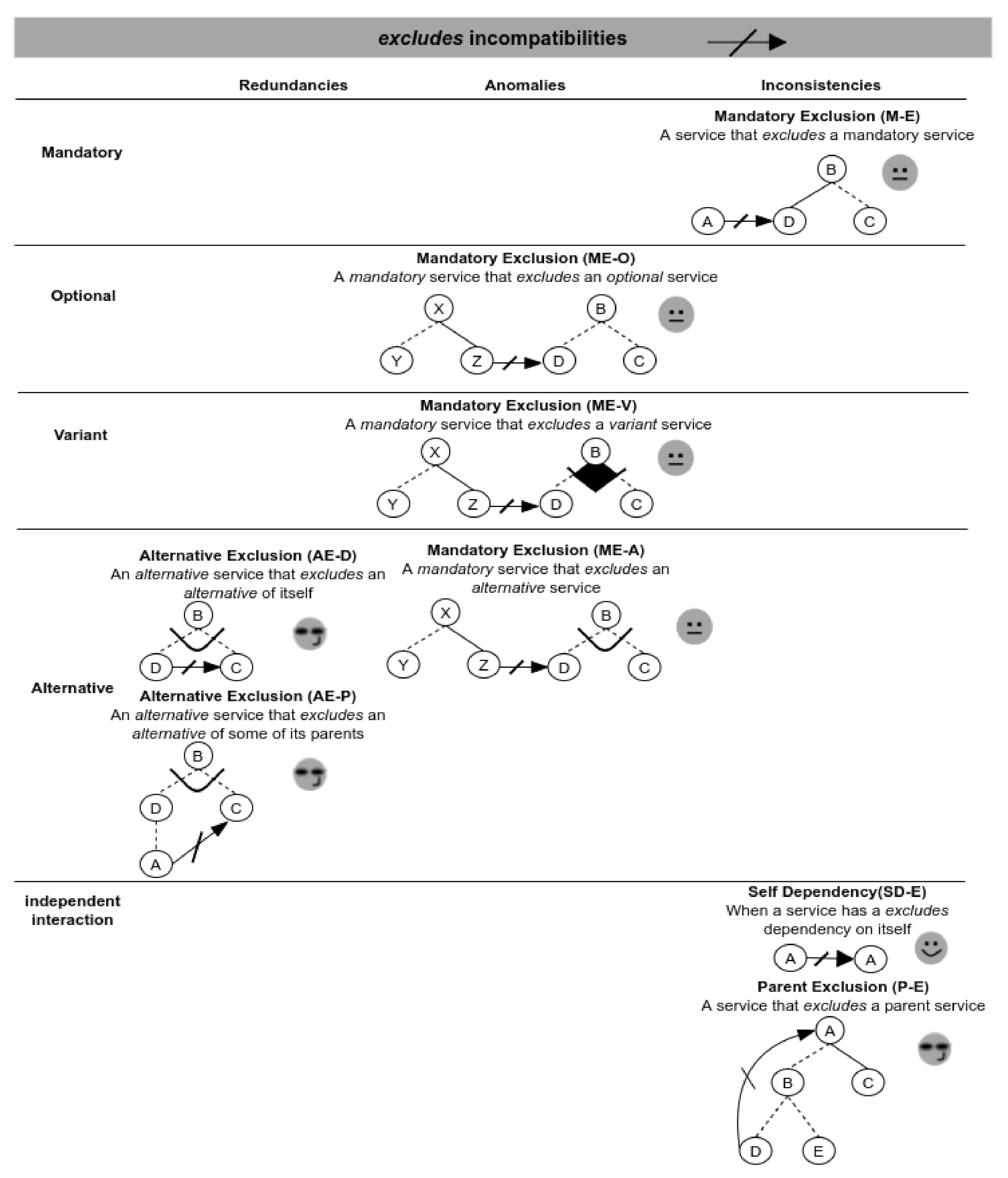
Following, Figure 10 shows incompatibilities when excludes dependencies are involved. Here, we have three possible inconsistencies in the scenarios—mandatory exclusion, self dependency and parent exclusion. At the same time, we can see that the responses of the validator are mostly warnings for alerting the exclusion of services on all instantiated products. For example, for the ME-A scenario, the validator uses the Mandatory_exclude(Z,D) function, which, given two services Z and D (where ), checks if D belongs to a mandatory variation point (Listing 2).
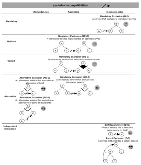
Figure 10.
Validation scenarios involving excludes incompatibilities.
Listing 2.
Mandatory_exclude(Z,D) function.
Listing 2.
Mandatory_exclude(Z,D) function.
 |
As mentioned above, the result of the evaluation is a warning about the presence of the scenario together with the involved services (Z and D).
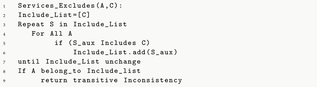
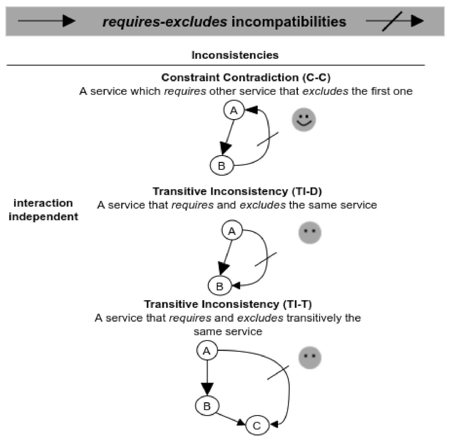
Figure 11 shows the validation scenarios involving both requires and excludes dependencies. In this case, all the scenarios present inconsistencies because they are involving services that are requiring and excluding the same services. Except for the C-C scenario, in which the validator can identify the specific services in conflict, the other two scenarios are only identified generally. For example, the TI-T scenario is evaluated by means of a Services_Excludes(A,C) function, which, given two services A and C (where ), generates a list (Includes_List) of all services that requireC; recursively adding services, which in turn require services that belong to the list (Includes_List). Then, if the service A belongs to Includes_List, there is a transitive inconsistency between A and C (Listing 3).
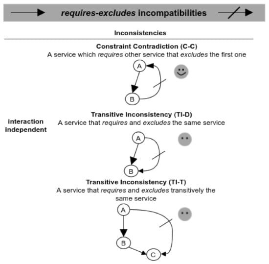
Figure 11.
Validation scenarios involving requires-excludes incompatibilities.
Listing 3.
Services_Excludes(A,C) function.
Listing 3.
Services_Excludes(A,C) function.
 |
The response of this evaluation is a general identification. The validator can only identify the involved services, but not the specific scenario.
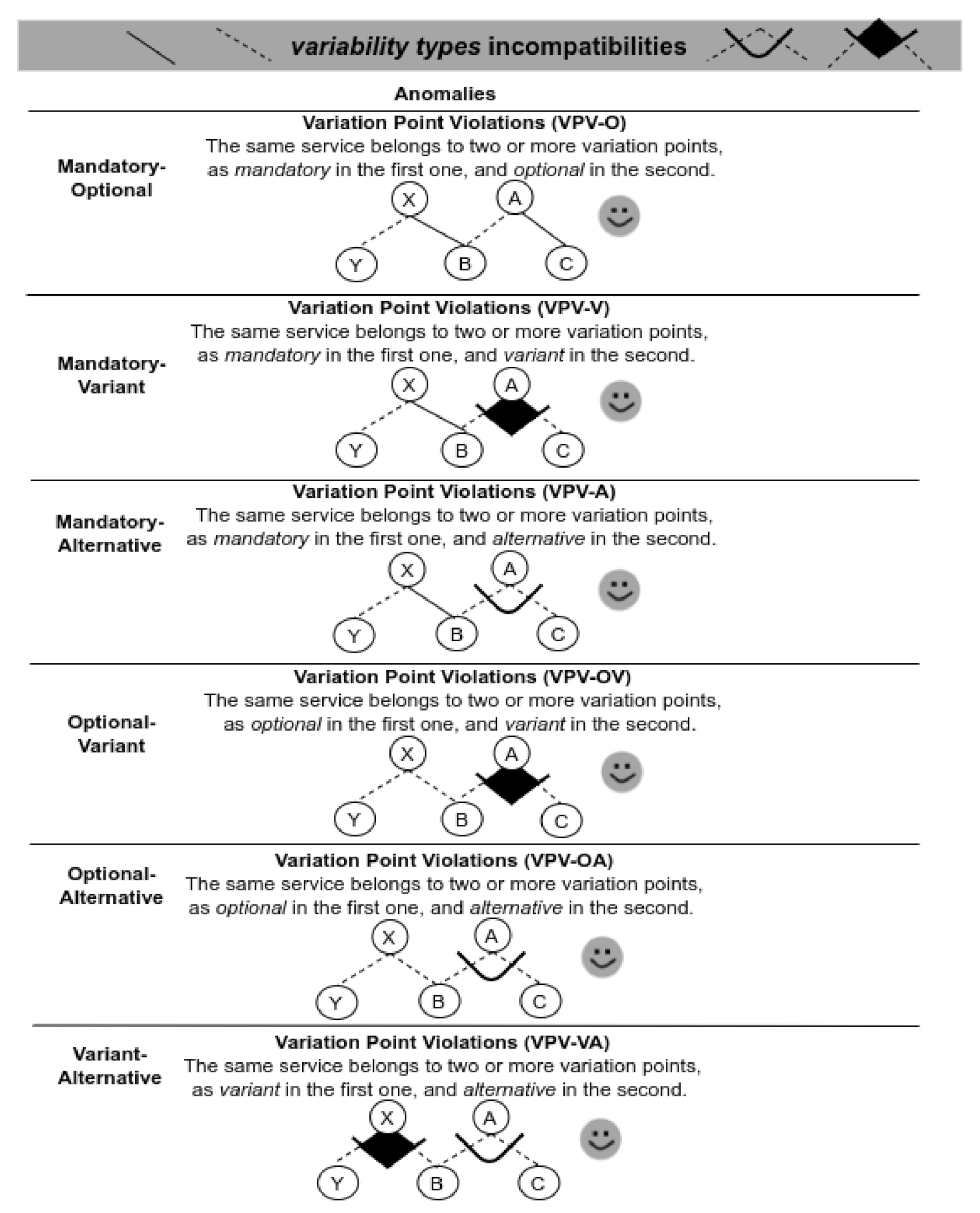
In Figure 12, we can see the validation scenarios involving combinations of variability types. These scenarios only generate anomalies, making services with specific associated variability cannot be really instantiated.
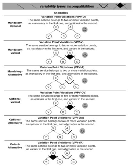
Figure 12.
Validation scenarios involving variability types incompatibilities.
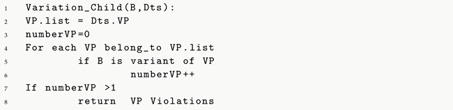
To evaluate these scenarios, we use the Variant_Child(B,Dts) function, which, given a variant B and a variability model , checks the number of variation points that the variant B contains. If the number of variation points is greater than one, there is a variation point violation (Listing 4).
Listing 4.
Variant_Child(B,Dts) function.
Listing 4.
Variant_Child(B,Dts) function.
 |
The response of the evaluation of these scenarios is a specific identification of the involved services in the anomaly.
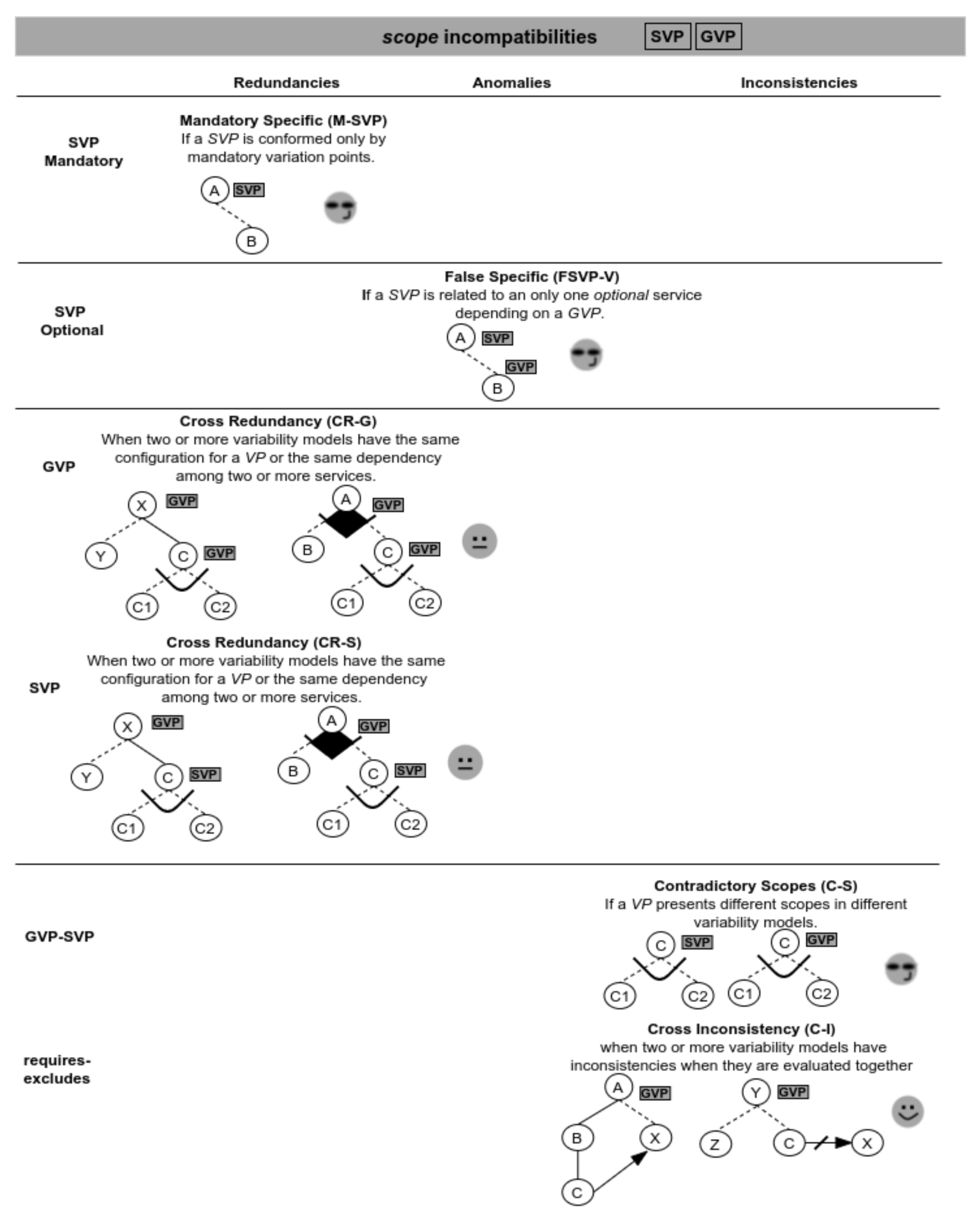
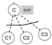
Finally, Figure 13 shows the validation scenarios involving scope operators. In these cases, there are possible redundancies involving the scope operators; therefore, it would be useful to know how to proceed with their instantiation. For instance, the M-SVP scenario is redundant because, regardless the instantiation you want to apply, the can never contain different configurations, so the validator suggests modifying the scope operator to .

Figure 13.
Validation scenarios involving scope incompatibilities.
Other redundancies occur in the CR-G and CR-S scenarios. For example, variability models in the figure are redundant considering the variation point C, because it is designed in the same way in both variability models. It is important to highlight here that these scenarios are not representing necessarily a problem, but it is useful for the designer that they are detected. Thus, the result of the evaluation is a warning about the presence of the scenario together with the involved services.
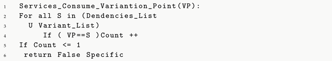
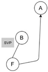
Following, an anomaly occurs in the FSVP-V scenario when a specific variation point SVP is related to an only one variant service depending on a GVP. When this happens, the scope will be always GVP because it is independent from the way the service is configured. This scenario is validated by using the Services_Consume_Variation_Point(VP) function, which given a variation point returns the number of services that use it; and when this number is one, we are in the presence of a False Specific (Listing 5).
Listing 5.
Services_Consume_Variation_Point(VP) function.
Listing 5.
Services_Consume_Variation_Point(VP) function.
 |
So, this variation point is suggested to be converted into a . Finally, we can see the C-S scenario representing an inconsistency when the same has different scopes in different variability models. To evaluate this scenario, for each service that represents a variation point, we register its scope into the underlying structures. Therefore, in the Service_Scope(S) function, when registering the scope, we check if the service has the same scope; in any other case, we are in the presence of a scope inconsistency (Listing 6).
Listing 6.
Service_Scope(S) function.
Listing 6.
Service_Scope(S) function.
 |
The result of the evaluation of this scenario suggests modifying the scope operator to .
As a summary of the validation scenarios and the responses of our validator, Figure 14 shows, for each incompatibility, the number of scenarios according to each type of response.

Figure 14.
Summary of number of validation scenarios according to the response of the validator.
Configurator (Component 3.2)
The configurator allows developers to build a specific product by means of instantiating the functional datasheets included in an SPL platform. Therefore, this component presents a user interface (UI) that allows developers to select the different variant services (associated with variation points). To perform that, a developer receives as input the validated functional datasheets (without anomalies), instantiates them, and generates a new set of datasheets without variability. This new set must be evaluated again.
4.4. The SeVaTax Web Tool
The SeVaTax process is supported by a Web tool that follows a layered model implemented as a client-server architecture. It is developed with the Angular (https://angular.io/) framework, and it is open-source (https://github.com/IngSisFAI/sevataxtool.git).
5. Validating the SeVaTax Process
In this section, we introduce two evaluations of the SeVaTax process aimed at validating accuracy and coverage of the scenarios. Figure 15 shows the process for designing the validation experiments, which is based on rules as activities defined in [39]. Once the hypotheses are defined (activity A), we carefully select the set of variability models to be analyzed, the solvers to be used, and the expected results. Finally, the experiments are run and the results analyzed.
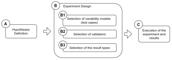
Figure 15.
Process for designing the validation experiments.
For the activity B1 (selection of variability models/test cases) we develop a tool that automatically generates variability models, taking into account the interactions defined in Table 1. This tool allows the designer to set up the number of variability models to be created, together with the number of services, variability points, dependencies, and levels for each of these models. Designers can also specify the number of inconsistencies or it can be set up as automatic. This tool is available to be downloaded from https://github.com/IngSisFAI/variabilityModelGenerator, and the test cases used in the next experiments are available from https://github.com/IngSisFAI/variabilityModelGenerator/tree/master/testCases.
5.1. Experiment 1: Accuracy
This evaluation analyzes accuracy when identifying specific incompatibilities through the use of scenarios. In this case, we compare our validator (component 3) to a basic implementation of an SAT solver (Sat4j).
- A.
- Hypotheses Definition
We define the following hypotheses:
Hypothesis 1 (H1).
A basic SAT solver is not enough for identifying specific incompatibilities of the variability models.
Hypothesis 2 (H2).
The SeVaTax validator improves incompatibility identification. This means that an incompatibility is not only identified but also the validator can identify the involved services and interactions.
- B.
- Experiment Design
Figure 16 shows the workflow for the experiment design. In the following, we describe each activity performed for validating accuracy.
B1. Selection of variability models: Here, we use our automatic variability model generation tool to create 30 test cases (variability models) containing 170 incompatibilities distributed into redundancies, anomalies and inconsistencies.
B2. Selection of validators: Each branch of the workflow, shown in Figure 16, represents a different validator. Thus, in the figure, we can see three branches: (1) the branch for the basic SAT solver, (2) the branch for validating our proposal, and (3) the manual validation in which the expected results are defined.
We choose a basic implementation of an SAT solver (Sat4j) because it is the same solver used by our approach. Similarly, in the figure we can see that the CNF translation is used as input of these two validators; but differently, our validation adds the inputs generated by the underlying structures used in the SeVaTax process.
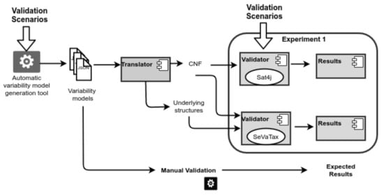
Figure 16.
Experiment 1—Workflow for accuracy validation.
Figure 16.
Experiment 1—Workflow for accuracy validation.

B3. Selection of the result types: The validation of the 30 test cases is performed by considering the next result types:
- (i)
- The validator identifies each validation scenario correctly.
- (ii)
- The validator finds some scenarios, but at least one of them is not correctly identified.
- (iii)
- The validator finds an error or problem but cannot identify the scenario.
- (iv)
- The validator cannot identify any scenario.
- C.
- Execution of the experiment and results
Figure 17 shows the expected results (third branch of Figure 16) in terms of the percentage of the number of scenarios (according to our test data) falling into each category. For example, for the 170 incompatibilities, 20% (34 incompatibilities) fall into requires incompatibilities (Figure 9), 30% (51 incompatibilities) are exclude incompatibilities (Figure 10), and so on.
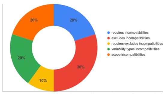
Figure 17.
Expected Results—Percentage of incompatibilities for each category.
In Figure 18 and Figure 19, we show the results for the basic SAT solver (first branch of Figure 16) and for the SeVaTax process (second branch of Figure 16), respectively, with respect to the expected values and the result types generated.
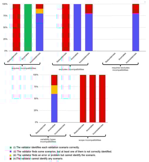
Figure 18.
Results obtained by the basic SAT solver implementation.

Figure 19.
Results obtained by the SeVaTax validator.
Thus, Figure 18 shows the percentage of each result type answered when test cases are analyzed with a basic SAT solver. For example, we can see that redundancies and scopes scenarios are not identified at all, that is 100% of (iv) responses (in red) (In case of require-excludes and variability types incompatibilities the bar of redundancies is 0% because these categories do not present any scenario of this type). These non-identified scenarios represent 56% of the total of scenarios according to the expected results (Redundancies scenarios are distributed among the categories (in Figure 17) containing this type of incompatibility). The scenario with the best result is FV (False Variability, which includes FV-O, FV-V and FV-A) representing anomalies within requires incompatibilities (Figure 9). In the figure we can see that this bar shows 100% of scenarios being identified correctly (response (i), in blue), and at the same time represents exactly 20% of the scenarios of test cases (according to Figure 17).
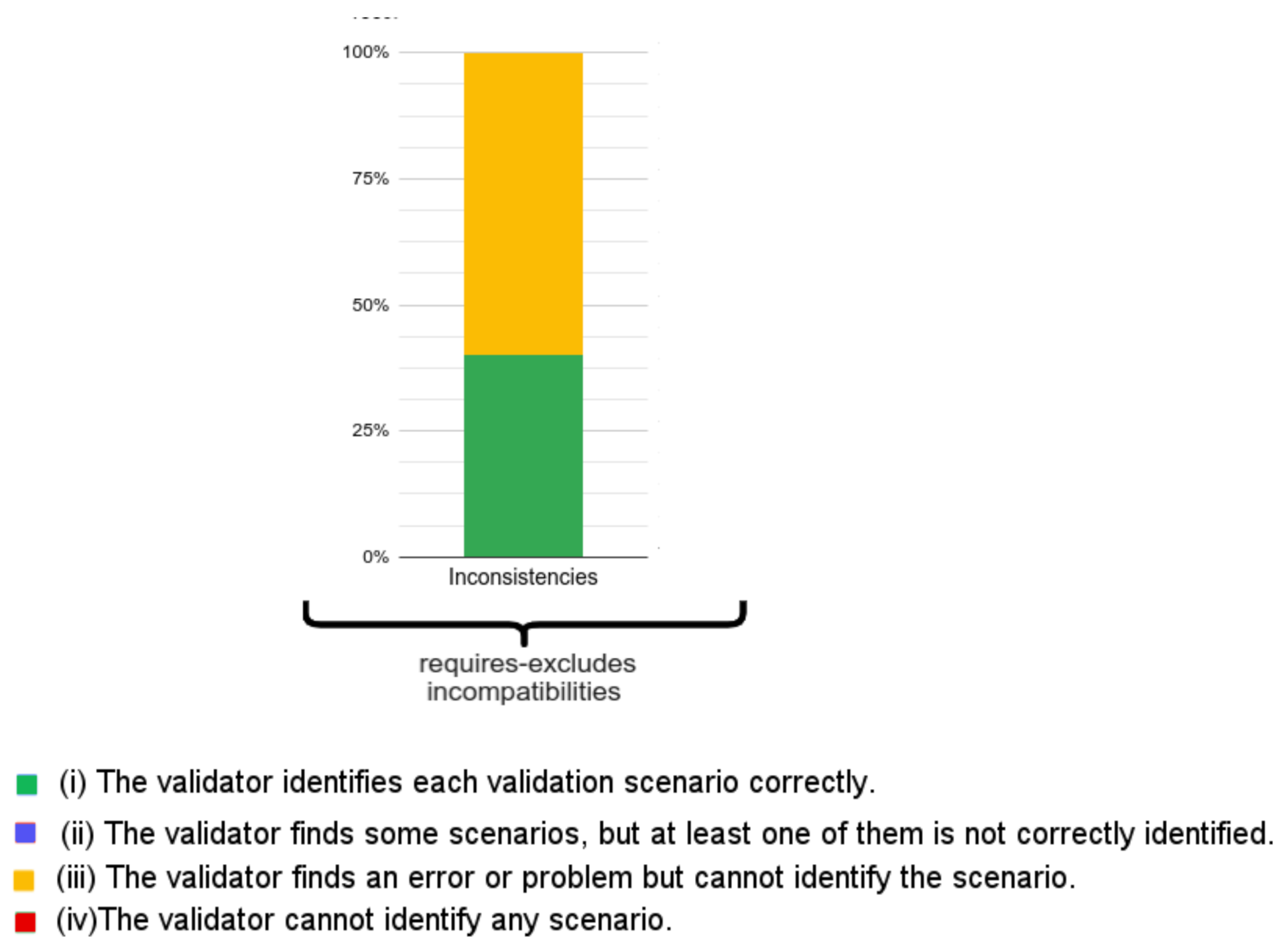
With respect to the SeVaTax validator, in Figure 19 we only show incompatibilities for which we obtained negative results, that is, when the scenarios fall into (ii), (iii) or (iv) results. This happens only in the TI scenarios (transitive inconsistency, which includes TI-T and TI-D scenarios) within requires-excludes incompatibilities (Figure 11). Here, SeVaTax cannot determine these specific incompatibilities, that is, it cannot identify the specific scenario generating the inconsistency. Sixty percent (in yellow in Figure 19) represent these cases, and the other 40% represent the C-C scenarios (within the requires-excludes incompatibilities according to Figure 11), in which SeVaTax identifies every incompatibility correctly. These scenarios represent 6% of the total of the analyzed scenarios (according to Figure 17, requires-excludes incompatibilities represent 10% of the scenarios, in which 6% are TI-T and TI-D, and the rest are C-C scenarios in which SeVaTax obtained an (i) result).
In summary, from the analysis of Figure 18 and Figure 19 we can see that the hypothesis H1 is confirmed with 45% of the non-identified scenarios for the basic SAT solver ((iv) responses). This percentage is comparable to the 6% of non-identified scenarios by the SeVaTax validator. Similarly, the hypothesis H2 is confirmed and reflected in the accuracy of the responses given by SeVaTax, that is, most of the responses fall into the (i) result.
5.2. Experiment 2: Coverage
This evaluation analyzes the coverage of the inconsistencies, anomalies and redundancies represented through the validation scenarios. We compare here SeVaTax against two other approaches: SPLOT and VariaMos. We choose these approaches based on two main aspects. Firstly, they are widely referenced in the literature with visible results, and secondly they provide configurable and available tools in which inputs and processing are well-defined.
- A.
- Hypotheses Definition
We define the following hypotheses:
Hypothesis 3 (H3).
The SeVaTax validator provides a specific answer for each validation scenario, that is, the validator has the ability to find the specific incompatibility (redundancy, anomaly and/or inconsistency) and classify it as a scenario.
Hypothesis 4 (H4).
The SeVaTax validator improves the identification of validation scenarios, providing better descriptions and solutions.
Both hypotheses are addressed to show that SeVaTax provides an improvement with respect to the correct identification of the validation scenarios and to the generation of specific responses.
- B.
- Experiment Design
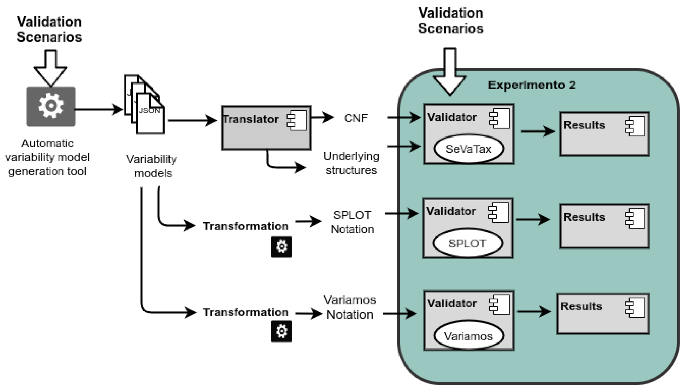
Figure 20 shows the workflow for the experiment design. Following we describe each activity performed by the coverage validation.
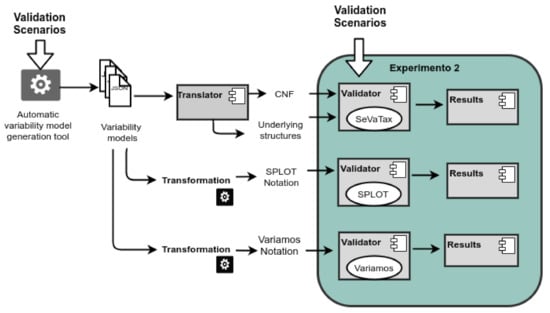
Figure 20.
Experiment 2—Workflow for coverage validation.
B1. Selection of variability models: Here, we use the automatic variability model generation tool to create 14 test cases with one validation scenario for each one. The scenarios associated to scope incompatibilities (Figure 13) are not considered here because scope operators are only proposed by our approach.
B2. Selection of validators: As we can see in Figure 20, we have three branches, one for each validator. Firstly, we translate the 14 variability models to the specific format expected by SPLOT and VariaMos. Both approaches use feature models as inputs, but also add specific characteristics. So, we manually translate the SeVaTax models to each notation.
B3. Selection of the result types: The validation of the 14 test cases is performed by considering the result types defined in the component Results of Figure 3: warning (W), identification (I), general identification (GI), and repair (R). We also add new responses for the analysis: (1) Not-Allowed (NA), when the inconsistency is not possible to be modeled by the approach, and (2) Not-Detected (ND) when neither the scenario or the problem is identified.
- C.
- Execution of the experiment and results
For the execution of this experiment, the 14 test cases, with the specific format of each approach, are run on each tool. Then, we analyze each result manually.
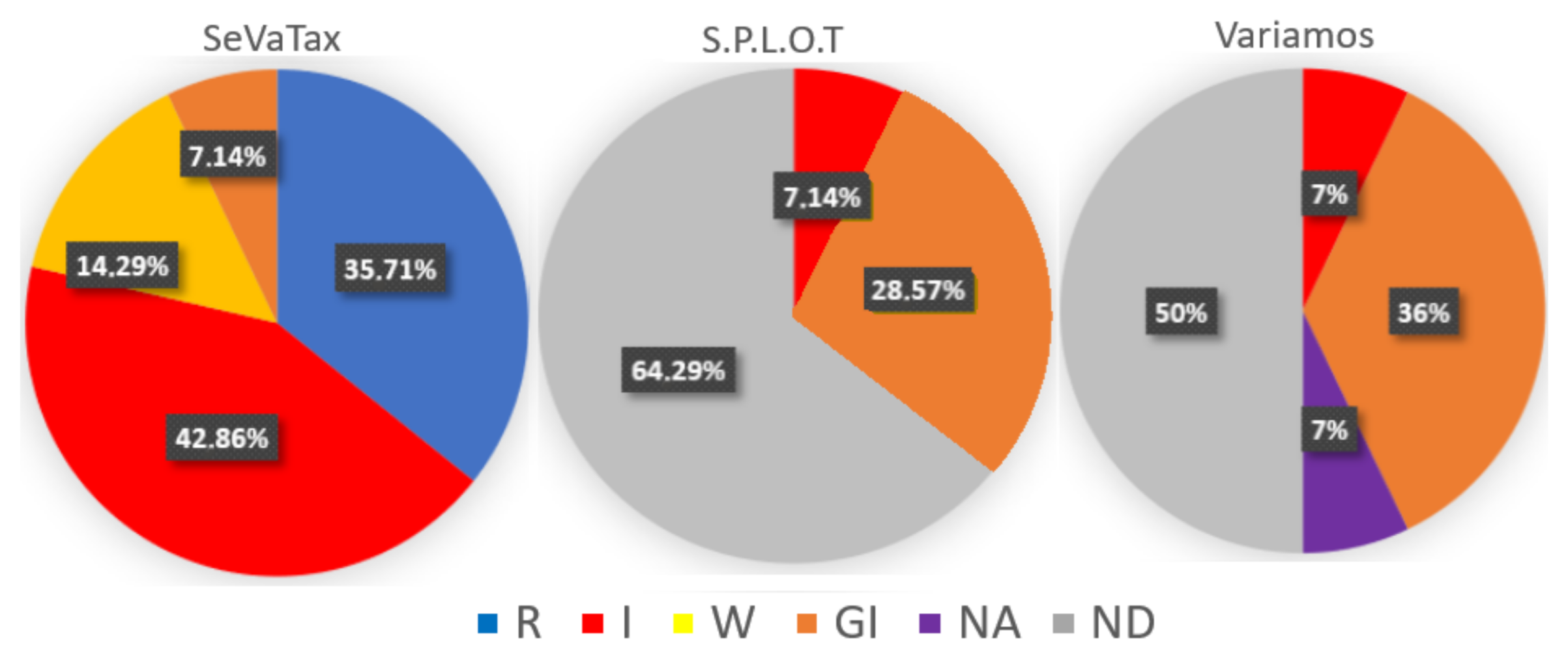
In Figure 21, we can observe that SPLOT identifies 35.71% (7.14% I and 28.57% GI) of the 14 scenarios. On the other hand, VariaMos has a coverage of 50% (7% I, 36% GI and 7% NA) of the 14 scenarios proposed, without considering the scope operators. Like SPLOT, VariaMos identifies inconsistencies in a general way (GI) and identifies (I) the false variability scenarios (included in requires incompatibilities). Furthermore, VariaMos does not allow us to model (NA) the SD-E scenario included in the excludes incompatibilities.

Figure 21.
Coverage percentage for each validation scenario according to the three validators.
The high percentages of unidentified scenarios (ND) in SPLOT (62.9%) and VariaMos (50%) are due in part to the little support that both approaches provide to scenarios with redundancies for all categories. As we have described previously, redundancies do not necessarily imply a logical inconsistency; however, they can present problems in the design and maintenance of the functionalities.
With respect to our approach, 92.79% of the 14 scenarios involved in the validation are identified, and even 35.7% are corrected (R). Only 7.14% of these 14 scenarios are generally identified and 14.29% generate an alert (W). This fact confirm the H3 hypothesis because our approach identifies and provides more specific responses, and even suggests corrections.
The results from Figure 21 validate the hypothesis H4, since the percentage of coverage is higher in SeVaTax compared to the other two approaches. In concordance, these approaches show a high percentage of validation scenarios that are not identified. This percentage is 64.29% in S.P.L.O.T, and 50% in VariaMos.
5.3. Threats to Validity
In [40], threats to validity are divided into four main categories for quantitative experimentation: conclusion validity for analyzing whether the experimental process is related to the outcomes found, internal validity for analyzing whether the experimental process really arrives to the outcomes found (there are no other factor that can affect the results), external validity for considering whether the results can be generalized, and construct validity for considering the relation between the theory behind the experimental process and the observations.
Looking at our experiments in the light of these threats, we found that each hypothesis was analyzed by using a well-defined and controlled validation process. Firstly, we have specially created an automatic variability model generation tool that randomly generates models with a specific number of inconsistencies and anomalies falling into the types of validation scenarios.
Then, in the case of our first experiment about accuracy, we used the same inputs, that is, the same variability models with the same CNF translation for both validators (Figure 16). So, we consider that there is no threat to internal or construct validity. As these variability models were generated by a software tool, there is no possibility of biases.
The conclusions of the experiment were based on a classification of result types according to each of the incompatibilities and expected responses. At this point, it is important to analyze the threats of conclusion validity in terms of the first three validations described (from (i) to (iii)). For example, we should analyze if these types of results are complete in terms of all possible answers, or if, in the case of the SAT solver, there are other types of answers that were not considered. As the validation scenarios were defined by ourselves, the experiment was guided towards these incompatibilities, even known that an SAT solver is not specifically designed to find such scenarios, so the answers depended on unexpected implementations. However, these implementations are valid situations of inconsistencies, anomalies or redundancies within variability models, so these problems must be detected. Another threat of conclusion validity is that the experiment was not applied and tested in a real context, but simulated with variability models.
Finally, we analyze the inputs of the expected results in the manual validation branch of Figure 16. As they were determined manually, it is possible for different people to determine different results. However, we had considered this situation, and the results were independently requested to different members of our research group, and analyzed together. In general, the results had very little variation and they were considered for generating the expected results we used.
Considering the second experiment, coverage, we can also analyze some threats to validity, in particular with respect to the inputs. Here, although the variability models were the same, we had to translate them to the specific format expected by each approach (SPLOT and VariaMos), and the translations were made manually. As each approach can slightly vary on modeling some variability primitives, we can have some differences among the inputs, which can affect the results. Thus, this fact can generate threats to conclusion validity.
Finally, considering the external validity of both experiments, we can analyze whether they can be generalized. In particular, as we have proposed a well-defined validation process (Figure 15) and conducting the experiments through controlled steps, we can change, for example, the set of validators applied on each experiment and run the same steps, even under the same hypotheses and result types. At the same time, as the automatic variability model generation tool is available to be downloaded, anyone can generate new inputs with new or the same validators.
6. Results
By considering the challenges and open issues obtained from the literature (Section 3), the SeVaTax process included artifacts and resources aimed at improving the activities involved in a VA process. Coming back to the challenges specifically addressed in this work, we discuss the way we proposed to deal with them as follows:
- Challenge 1: Define the set of basic operations (queries) that the VA process must support. Here, we have defined an extensive set of validation scenarios (31 scenarios) including a wide number of incompatibilities, which consider redundancies, anomalies and inconsistencies that can be present in the variability models. These scenarios have been obtained from the literature and from our experiences in the development of two SPLs for the marine ecology [35,36] and paleontology [38] domains. Specifically, from these developments we included the scope operators for reusing variation points and their instantiations. At the same time, we added specific support for each defined scenario, not only for a general identification, but also as a specific description of the services involved; and in the cases in which it is possible, we suggested corrections;
- Challenge 2: Include extended variability primitives together with their specific operations. At this point, as we use the OVM notation together with UML artifacts oriented to functional-based design models, we have extended the variability primitives of these models with scope operators. These operators emerged from an application of the SeVaTax models in GIS systems [37], where we needed ways to relate the same variability points distributed in several variability models. These operators let us to represent the real semantic of the domains;
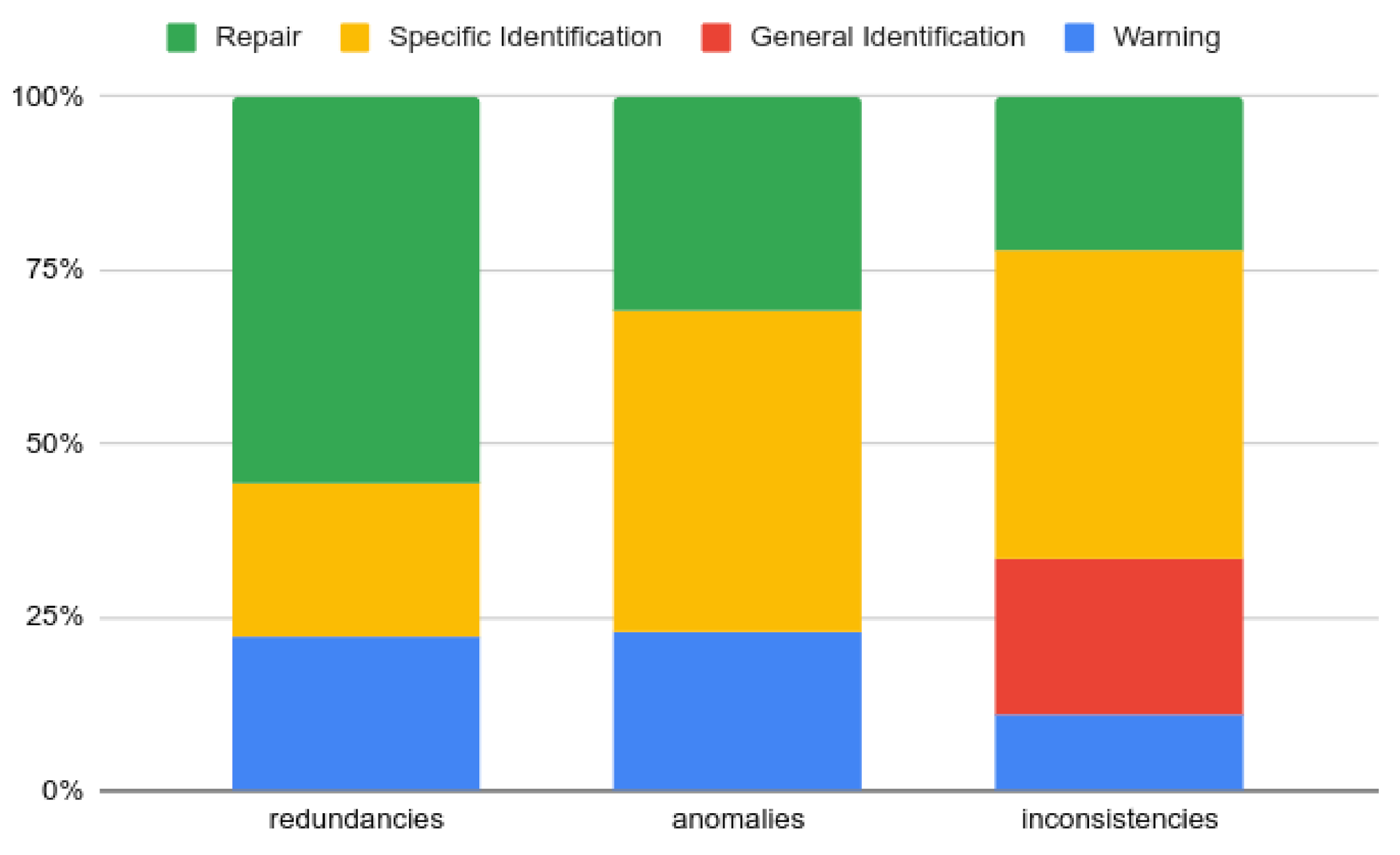
- Challenge 3: Addition of more support for error correction. The SeVaTax process contains a set of different responses (warnings, identifications, and/or reparations) when analyzing the variability models. As a summary, in Figure 14 we showed the responses generated by SeVaTax with respect to each incompatibility. In Figure 22 we also can see a summary of responses with respect to the severity level (redundancies, anomalies and inconsistencies) of the incompatibility. We can see that our validator repairs 50.5% of redundancies, 30.7% of anomalies, and 22.2% of inconsistencies. The response most regularly generated is the specific identification with 38% of the incompatibilities. The second one is repair (error correction), representing 35% of the incompatibilities;
 Figure 22. Summary of responses with respect to the severity level.
 - Challenge 4: Addition of most rigorous evaluations. Here, we have performed two experiments for validating accuracy and coverage. In the first one, we evaluated the quality of the responses in the SeVaTax process with respect to a manual response and a basic SAT solver. In the second experiment, we evaluated the coverage of the validation scenarios, that is, the capacity of different solvers to detect and respond to specific anomalies, incompatibilities, and redundancies.
7. Conclusions
In this work, we have briefly described our approach for the automated analysis of variability models, called SeVaTax. Then, we have extended the SeVaTax process, presented in previous works, in order to face some challenges defined in this field. As extensions, we have focused on improving validation scenario definitions (queries) and validation support (by solvers and underlying structures) in order to provide more concise results. In addition, we have performed two evaluations for analyzing the accuracy and coverage of the SeVaTax process.
However, there are still challenges that have not been addressed by our approach and must be taken into account in future work. One of them is the need for industrial validations, which empirically evaluate the cost and effort of using our tool. In this sense, we are currently working on running experiments in the paleontology domain, focusing on analyzing acceptance and effort.
Author Contributions
Conceptualization, A.B. and A.C.; Investigation, M.P., A.B. and A.C.; Methodology, M.P. and A.B.; Software, M.P.; writing—original draft preparation, A.B.; writing—review and editing, A.C.; supervision, A.B. All authors have read and agreed to the published version of the manuscript.
Funding
This research received no external funding.
Institutional Review Board Statement
Not applicable.
Informed Consent Statement
Not applicable.
Data Availability Statement
The SeVaTax process is supported by a Web tool developed with the Angular (https://angular.io/) framework: (https://github.com/IngSisFAI/sevataxtool.git). Additionally, for the evaluations, we develop a tool that automatically generates variability models. This tool is available to be downloaded from https://github.com/IngSisFAI/variabilityModelGenerator, and the test cases used in the experiments are available from https://github.com/IngSisFAI/variabilityModelGenerator/tree/master/testCases.
Acknowledgments
This work is partially supported by the UNComa project 04/F009 “Reuso de Software orientado a Dominios—Parte II” part of the program “Desarrollo de Software Basado en Reuso—Parte II”.
Conflicts of Interest
The authors declare no conflict of interest.
Abbreviations
The following abbreviations are used in this manuscript:
| VA | Variability Analysis |
| SPL | Software Product Line |
| FM | Feature Models |
| OVM | Orthogonal Variability Model |
| CVL | Common Variability Language |
| CSP | Constraint Satisfaction Problem |
| CNF | Conjunctive Normal Form |
| DL | Description Logic |
| CNF | Conjunctive Normal Form |
| TVML | Textual Variability Modeling Languages |
References
- Mazo, R.; Munoz-Fernandez, J.C.; Rincon, L.; Salinesi, C.; Tamura, G. VariaMos: An extensible tool for engineering (dynamic) product lines. In Proceedings of the 19th International Software Product Line Conference, Nashville, TN, USA, 20–24 July 2015; pp. 374–379. [Google Scholar] [CrossRef]
- Wang, H.H.; Li, Y.F.; Sun, J.; Zhang, H.; Pan, J. Verifying feature models using OWL. Web Semant. Sci. Serv. Agents World Wide Web 2007, 5, 117–129. [Google Scholar] [CrossRef]
- Benavides, D.; Segura, S.; Ruiz-Cortés, A. Automated Analysis of Feature Models 20 Years Later: A Literature Review. Inf. Syst. 2010, 35, 615–636. [Google Scholar] [CrossRef] [Green Version]
- Kang, K.; Cohen, S.; Hess, J.; Nowak, W.; Peterson, S. Feature-Oriented Domain Analysis (FODA) Feasibility Study; Technical Report CMU/SEI-90-TR-21; Software Engineering Institute, Carnegie Mellon University: Pittsburgh, PA, USA, 1990. [Google Scholar]
- Pohl, K.; Böckle, G.; Linden, F.J.v.d. Software Product Line Engineering: Foundations, Principles and Techniques; Springer: Secaucus, NJ, USA, 2005. [Google Scholar]
- Haugen, O.; Møller-Pedersen, B.; Oldevik, J.; Olsen, G.K.; Svendsen, A. Adding Standardized Variability to Domain Specific Languages. In Proceedings of the 2008 12th International Software Product Line Conference, 2008, Limerick, Ireland, 8–12 September 2008; pp. 139–148. [Google Scholar] [CrossRef]
- Pol’la, M.; Buccella, A.; Cechich, A. Analysis of variability models: A systematic literature review. Softw. Syst. Model. 2020, 20, 1043–1077. [Google Scholar] [CrossRef]
- Pol’la, M.; Buccella, A.; Cechich, A. Automated Analysis of Variability Models: The SeVaTax Process. In Proceedings of the Computational Science and Its Applications—ICCSA 2018—18th International Conference, Melbourne, Australia, 2–5 July 2018; Part IV. pp. 365–381. [Google Scholar] [CrossRef]
- Pol’la, M.; Buccella, A.; Cechich, A. Using Scope Scenarios to Verify Multiple Variability Models. In Proceedings of the Computational Science and Its Applications—ICCSA 2019—19th International Conference, Saint Petersburg, Russia, 1–4 July 2019; Lecture Notes in Computer Science, Part V. Volume 11623, pp. 383–399. [Google Scholar] [CrossRef]
- Braun, G.A.; Pol’la, M.; Cecchi, L.A.; Buccella, A.; Fillottrani, P.R.; Cechich, A. A DL Semantics for Reasoning over OVM-based Variability Models. In Proceedings of the 30th International Workshop on Description Logics, Montpellier, France, 18–21 July 2017; CEUR Workshop Proceedings. Volume 1879. [Google Scholar]
- Buccella, A.; Pol’la, M.; de Galarreta, E.R.; Cechich, A. Combining Automatic Variability Analysis Tools: An SPL Approach for Building a Framework for Composition. In Proceedings of the Computational Science and Its Applications—ICCSA 2018—18th International Conference, Melbourne, Australia, 2–5 July 2018; Lecture Notes in Computer Science. Volume 10963, pp. 435–451. [Google Scholar] [CrossRef]
- Eichelberger, H.; Schmid, K. A Systematic Analysis of Textual Variability Modeling Languages. In Proceedings of the 17th International Software Product Line Conference; SPLC’13; ACM: New York, NY, USA, 2013; pp. 12–21. [Google Scholar] [CrossRef]
- Lisboa, L.B.; Garcia, V.C.; Lucrédio, D.; de Almeida, E.S.; de Lemos Meira, S.R.; de Mattos Fortes, R.P. A systematic review of domain analysis tools. Inf. Softw. Technol. 2010, 52, 1–13. [Google Scholar] [CrossRef]
- Sree-Kumar, A.; Planas, E.; Clariso, R. Analysis of Feature Models Using Alloy: A Survey. In Proceedings of the 7th International Workshop on Formal Methods and Analysis in Software Product Line Engineering, FMSPLE@ETAPS 2016, Eindhoven, The Netherlands, 3 April 2016; pp. 46–60. [Google Scholar] [CrossRef] [Green Version]
- Jackson, D. Software Abstractions: Logic, Language, and Analysis; The MIT Press: Cambridge, MA, USA, 2006. [Google Scholar]
- Trinidad, P.; Benavides, D.; Cortés, A.R.; Segura, S.; Jimenez, A. FAMA Framework. In Proceedings of the International Software Product Line Conference, Washington, DC, USA, 8–12 September 2008; IEEE Computer Society: New York, NY, USA, 2008; p. 359. [Google Scholar]
- Krieter, S.; Pinnecke, M.; Krüger, J.; Sprey, J.; Sontag, C.; Thüm, T.; Leich, T.; Saake, G. FeatureIDE: Empowering Third-Party Developers. In Proceedings of the 21st International Systems and Software Product Line Conference—Volume B, Sevilla, Spain, 25–29 September 2017; SPLC ’17. ACM: New York, NY, USA, 2017; pp. 42–45. [Google Scholar] [CrossRef]
- Mendonca, M.; Branco, M.; Cowan, D. S.P.L.O.T.: Software Product Lines Online Tools. In Proceedings of the 24th ACM SIGPLAN Conference Companion on Object Oriented Programming Systems Languages and Applications, Orlando, FL, USA, 25–29 October 2009; pp. 761–762. [Google Scholar] [CrossRef]
- Roos-Frantz, F.; Galindo, J.A.; Benavides, D.; Ruiz-Cortés, A. FaMa-OVM: A tool for the automated analysis of OVMs. In Proceedings of the 6th International Software Product Line Conference—Volume 2, Leicester, UK, 6–11 September 2021; pp. 250–254. [Google Scholar]
- Sinnema, M.; Deelstra, S. Industrial validation of COVAMOF. J. Syst. Softw. 2008, 81, 584–600. [Google Scholar] [CrossRef]
- Dhungana, D.; Tang, C.; Weidenbach, C.; Wischnewski, P. Automated Verification of Interactive Rule-based Configuration Systems. In Proceedings of the 28th IEEE/ACM International Conference on Automated Software Engineering, Silicon Valley, CA, USA, 11–15 November 2013; ASE’13. IEEE Press: Piscataway, NJ, USA, 2013; pp. 551–561. [Google Scholar] [CrossRef]
- Classen, A.; Boucher, Q.; Heymans, P. A text-based approach to feature modelling: Syntax and semantics of TVL. Sci. Comput. Program. 2011, 76, 1130–1143. [Google Scholar] [CrossRef]
- Metzger, A.; Pohl, K.; Heymans, P.; Schobbens, P.; Saval, G. Disambiguating the Documentation of Variability in Software Product Lines: A Separation of Concerns, Formalization and Automated Analysis. In Proceedings of the 15th IEEE International Requirements Engineering Conference (RE 2007), New Delhi, India, 15–19 October 2007; pp. 243–253. [Google Scholar] [CrossRef] [Green Version]
- Cuenca, G.B.; Horrocks, I.; Motik, B.; Bijan, P.; Patel-Schneider, P.; Sattler, U. OWL 2: The Next Step for OWL. Web Semant. 2008, 6, 309–322. [Google Scholar]
- Rincón, L.; Giraldo, G.; Mazo, R.; Salinesi, C. An Ontological Rule-Based Approach for Analyzing Dead and False Optional Features in Feature Models. Electron. Notes Theor. Comput. Sci. 2014, 302, 111–132. [Google Scholar] [CrossRef] [Green Version]
- Langermeier, M.; Rosina, P.; Oberkampf, H.; Driessen, T.; Bauer, B. Management of Variability in Modular Ontology Development. In Service-Oriented Computing—ICSOC Workshops; Lomuscio, A., Nepal, S., Patrizi, F., Benatallah, B., Brandić, I., Eds.; Springer International Publishing: Cham, Switzerland, 2014; pp. 225–239. [Google Scholar]
- Afriyanti, I.; Falakh, F.; Azurat, A.; Takwa, B. Feature Model-to-Ontology for SPL Application Realisation. arXiv 2017, arXiv:1707.02511. [Google Scholar]
- Von Der Massen, T.; Lichter, H. Deficiencies in Feature Models. Available online: http://www.soberit.hut.fi/SPLC-WS/AcceptedPapers/Massen.pdf (accessed on 21 December 2021).
- Nakajima, S. Semi-automated Diagnosis of FODA Feature Diagram. In Proceedings of the 2010 ACM Symposium on Applied Computing, Sierre, Switzerland, 22–26 March 2010; SAC ’10. ACM: New York, NY, USA, 2010; pp. 2191–2197. [Google Scholar] [CrossRef]
- Wang, B.; Xiong, Y.; Hu, Z.; Zhao, H.; Zhang, W.; Mei, H. Interactive Inconsistency Fixing in Feature Modeling. J. Comput. Sci. Technol. 2014, 29, 724–736. [Google Scholar] [CrossRef]
- Bilic, D.; Carlson, J.; Sundmark, D.; Afzal, W.; Wallin, P. Detecting Inconsistencies in Annotated Product Line Models. In Proceedings of the 24th ACM Conference on Systems and Software Product Line: Volume A, SPLC ’20, Montreal, QC, Canada, 19–23 October 2020; Association for Computing Machinery: New York, NY, USA, 2020. [Google Scholar]
- Horcas, J.M.; Galindo, J.A.; Heradio, R.; Fernandez-Amoros, D.; Benavides, D. Monte Carlo Tree Search for Feature Model Analyses: A General Framework for Decision-Making. In Proceedings of the 25th ACM International Systems and Software Product Line Conference—Volume A, Leicester, UK, 6–11 September 2021; Association for Computing Machinery: New York, NY, USA, 2021; pp. 190–201. [Google Scholar]
- Beek, M.H.t.; Mazzanti, F.; Damiani, F.; Paolini, L.; Scarso, G.; Lienhardt, M. Static Analysis and Family-Based Model Checking with VMC. In Proceedings of the 25th ACM International Systems and Software Product Line Conference—Volume A, Leicester, UK, 6–11 September 2021; Association for Computing Machinery: New York, NY, USA, 2021; p. 214. [Google Scholar]
- Fu, M.C. Monte Carlo tree search: A tutorial. In Proceedings of the 2018 Winter Simulation Conference (WSC), Gothenburg, Sweden, 9–12 December 2018; pp. 222–236. [Google Scholar] [CrossRef]
- Buccella, A.; Cechich, A.; Arias, M.; Pol’la, M.; del Socorro Doldan, M.; Morsan, E. Towards systematic software reuse of GIS: Insights from a case study. Comput. Geosci. 2013, 54, 9–20. [Google Scholar] [CrossRef]
- Buccella, A.; Cechich, A.; Pol’la, M.; Arias, M.; Doldan, S.; Morsan, E. Marine Ecology Service Reuse through Taxonomy-Oriented SPL Development. Comput. Geosci. 2014, 73, 108–121. [Google Scholar] [CrossRef]
- Brisaboa, N.R.; Cortiñas, A.; Luaces, M.; Pol’la, M. A Reusable Software Architecture for Geographic Information Systems Based on Software Product Line Engineering. In Model and Data Engineering; Bellatreche, L., Manolopoulos, Y., Eds.; Springer International Publishing: Cham, Switzerland, 2015; pp. 320–331. [Google Scholar]
- Buccella, A.; Cechich, A.; Porfiri, J.; Diniz Dos Santos, D. Taxonomy-Oriented Domain Analysis of GIS: A Case Study for Paleontological Software Systems. ISPRS Int. J. Geo-Inf. 2019, 8, 270. [Google Scholar] [CrossRef] [Green Version]
- Wohlin, C.; Runeson, P.; Höst, M.; Ohlsson, M.C.; Regnell, B.; Wesslén, A. Experimentation in Software Engineering: An Introduction; Kluwer Academic Publishers: Norwell, MA, USA, 2000. [Google Scholar]
- Wohlin, C.; Runeson, P.; Hst, M.; Ohlsson, M.C.; Regnell, B.; Wessln, A. Experimentation in Software Engineering; Springer International Publishing: New York, NY, USA, 2012. [Google Scholar]


Publisher’s Note: MDPI stays neutral with regard to jurisdictional claims in published maps and institutional affiliations. |
© 2022 by the authors. Licensee MDPI, Basel, Switzerland. This article is an open access article distributed under the terms and conditions of the Creative Commons Attribution (CC BY) license (https://creativecommons.org/licenses/by/4.0/).