Article

Parallel Particle Swarm Optimization Using Apache Beam

1
Computer School, University of South China, Hengyang 421001, China
2
Science and Technology on Parallel and Distributed Processing Laboratory (PDL), National University of Defense Technology, Changsha 410073, China
*
Author to whom correspondence should be addressed.
Information 2022, 13(3), 119; https://doi.org/10.3390/info13030119
Submission received: 7 January 2022 / Revised: 22 February 2022 / Accepted: 24 February 2022 / Published: 28 February 2022
(This article belongs to the Topic Big Data and Artificial Intelligence)

Abstract

:
The majority of complex research problems can be formulated as optimization problems. Particle Swarm Optimization (PSO) algorithm is very effective in solving optimization problems because of its robustness, simplicity, and global search capabilities. Since the computational cost of these problems is usually high, it has been necessary to develop optimization algorithms with parallelization. With the advent of big-data technology, such problems can be solved by distributed parallel computing. In previous related work, MapReduce (a programming model that implements a distributed parallel approach to processing and producing large datasets on a cluster) has been used to parallelize the PSO algorithm, but frequent file reads and writes make the execution time of MRPSO very long. We propose Apache Beam particle swarm optimization (BPSO), which uses Apache Beam parallel programming model. In the experiment, we compared BPSO and PSO based on MapReduce (MRPSO) on four benchmark functions by changing the number of particles and optimizing the dimensions of the problem. The experimental results show that, as the number of particles increases, MRPSO remains largely constant when the number of particles is small (<1000), while the time required for algorithm execution increases rapidly when the number of particles exceeds a certain amount (>1000), while BPSO grows slowly and tends to yield better results than MRPSO. As the dimensionality of the optimization problem increases, BPSO can take half the time of MRPSO and obtain better results than it does. MRPSO requires more execution time than BPSO, as the problem complexity varies, but both MRPSO and BPSO are not very sensitive to problem complexity. All program code and input data are uploaded to GitHub.

1. Introduction

It is common for the real world to have a lot of optimization problems that are complex, large-scale, and NP-Hard. A lot of these problems not only contain constraints and objectives, but also have their modeling constantly changing. Unfortunately, it is hard for a universal method to provide a solution.
Nowadays, more and more artificial intelligence methods (e.g., heuristics and metaheuristics) are used to solve such problems in many different domains, such as online learning [1], multi-objective optimization [1,2], scheduling [3], transportation [4], medicine [5], data classification [6], etc. Many issues can theoretically be solved by searching through a large number of possible answers intelligently. For the metaheuristic algorithm, the search can begin with some type of guessing and then gradually refine the guesses until no further refinement is possible. The process of this can be seen as a blind climb: we start our search at a random point on the mountain and then, by jumping or stepping, keep moving upward until we reach the top.
The particle swarm optimization algorithm [7], a classical metaheuristic, has proven to be very effective in many fields [8,9,10]; it is a method for optimizing a problem by iteratively improving a candidate solution relative to a given measure of quality. During PSO, each particle has a velocity and position, and the optimization problem is transformed into several optimization functions, called fitness functions. Each particle records its own best value and updates the swarm’s best value.
In order to solve increasingly complex optimization problems, a useful method is parallel PSO. The parallelization solutions include Hadoop MapReduce, MATLAB parallel computing toolbox, CUDA, R Parallel package, Julia: Parallel for and MapReduce, OpenGL, OpenCL, OpenMP with C++ and Rcpp, Parallel computing module in python, MPI, HPF, PVM, POSIX threads, and Java threads on SMP machines [11].
Previous papers [12,13] have implemented MapReduce parallel PSO, which proved to be very effective in training a radial basis function (RBF) network and enlarging the swarm population and problem dimension sizes.
In this study, we used Apache Beam to implement parallelized PSO, as it is an open-source unified model for defining both batch and streaming data-parallel processing pipelines [14]. In the experiment, we used Apache Beam to parallelize the PSO algorithm (BPSO) and compare it with the running time and results of MapReduce parallel PSO (MRPSO).
In Section 2, we introduce the details of the PSO algorithm. In Section 3, we introduce the basic concepts of Apache Beam, WordCount programming examples, and the advantages of Apache Beam. In Section 4, we introduce, in detail, the algorithm ideas and steps of Apache Beam PSO. In Section 5, we compare BPSO with MRPSO on four benchmark functions, namely Sphere, Generalized Griewank, Generalized Rastrigin, and Rosenbrock functions, by varying the number and dimensionality of particles. The experiments show that BPSO can run faster and obtain better results than MRPSO under the same conditions. Finally, we summarize the paper and give directions for future work in Section 6.

2. Particle Swarm Optimization

PSO was originally proposed by Kennedy, Eberhart, and Shi [7,15] and was first developed to simulate social behavior [16], using formulas to mimic the movements of a bench of birds and fish.
In PSO, each particle updates its speed and position according to the best value found by itself and the best value found by the particle swarm, gradually approaching the global optimal value. Initially, each particle initializes its velocity and position in a function-specific feasible region and calculates its fitness by applying a fitness function. Then, the particle updates its speed and position by using the following equation [17]:
V i , d = C ( V i , d + C 1 R p ( P _ best i , d P i , d ) + C 2 R g ( G _ best i , d P i , d ) )
X i , d = X i , d + V i , d
the V is the particle’s velocity, i is the particle’s number in the swarm, d represents the dimension of the particle, and R p and R g are uniformly distributed random numbers.
In addition, P_best represents the best-known position of the particle and G_best is the best-known position of the entire swarm. C is a constriction factor derived from the existing constants in Equation (1):
C = 2 2 φ φ 2 4 φ
φ = C 1 + C 2
where C 1 = C 2 = 2.05.
Finally, if the particle’s fitness value is better, it updates P_best and G_best to the current position. When this is finished, the particle swarm has finished one iteration and is ready to go on to the next. The update process is summarized in Algorithm 1.
Algorithm 1. PSO Algorithm Update Process.
while a termination criterion is not met:
   for each particle i in the swarm:
     for each dimension:
        Update the particle’s velocity using Equation (1)
        Update the particle’s position using Equation (2)
     if f(Pi) better than f( P _ best i):
        Update the particle’s best known position
     if f( P _ best i) better than f( G _ best i):
        Update the swarm’s best known position
As PSO uses iteration to update the solutions, when will it stop? The termination criterion can be the number of iterations performed or a solution where the adequate objective function value is found [17].
PSO belongs to the field of swarm intelligence, so that it can be expressed in parallel. In combination with big-data models, such as MapReduce [12,13] Apache Spark [18,19], etc., the algorithm running speed can be improved further.

3. Apache Beam

Apache Beam is an open-source unified model for defining both batch and streaming data-parallel processing pipelines; it was created by language-specific SDKs and subsequently executed by one of the distributed back-ends supported by Beam, which includes Apache Nemo, Apache Flink, Hazelcast Jet, Apache Spark, Apache Samza, Twister2, and Google Cloud Dataflow [14].

3.1. WordCount

In Apache beam, the user’s program is a Pipeline (managing a directed acyclic graph of PTransforms and PCollections that is ready for execution [20]) and the input data are divided as PCollection (representing a collection of data, which could be bounded or unbounded in size [20]), which is transformed by PTransform (representing a computation that transforms input PCollections into output PCollections [20]). The PTransform can change, filter, group, analyze, or otherwise deal with elements in a PCollection. Then, we use IOs to the result to an external source. With the Runner (specifying where and how the pipeline should execute [20]) supported by the Apache Beam, we can run the pipeline without changing the code.
The flowchart of the classical WordCount program is shown in Figure 1, below.
As can be seen from the picture above, in the beginning, an input file is read by the Pipeline object and outputs a PCollection whose elements consist of lines of text. The transformation then splits the rows in the PCollection, where each element is a separate word. When the output of the previous step is received, the Count provided by the SDK converts it and outputs a PCollection of key/value pairs, where each key represents a unique word in the text, and the associated value is the number of occurrences of each key. The following conversion formats each key/value pair into a printable string that is suitable for writing to the output file. Finally, the Write conversion writes the string to the file.

3.2. Benefits of Apache Beam

With the development of big-data technology, a programming model called MapReduce can be used to solve the optimization problem of parallel PSO [12,13]. In addition, a MapReduce program usually consists of a mapping process (used to filter or sort data) and a reduction method (used to collect data to generate results).
However, the MapReduce task must be written as an acyclic data-flow program, that is, a stateless mapper followed by a stateless reducer, which is executed by the batch job scheduler [21]. Therefore, it is difficult to repeatedly query the dataset and solve optimization problems through iterative calculations. In addition, the algorithm is very slow when iterating, because it must save the data to the disk and reread the data from the disk for each iteration.
In order to overcome the abovementioned shortcomings, Apache Beam appeared, which unifies batch processing and stream data-parallel processing. The Apache Beam program is a pipeline, and data flow in the pipeline similar to water. We can use PTransform to transform the data into the format we need. With the rapid development of big data, more and more engines for large-scale data analysis appear, such as Apache Nemo, Apache Spark, Apache Flink, Google Cloud Dataflow, etc. While changing the big-data engine, we must relearn new languages and grammar, which wastes a lot of time and energy. In Apache Beam, we only need to care about the following four issues: What results are being calculated? Where in event time? When in processing time? How do refinements of results relate? We do not have to understand all the details of various runners and their implementations; instead, we need to focus on the logical composition of our data-processing jobs, rather than the physical orchestration of parallel processing.
The model behind Beam evolved from Google FlumeJava, MapReduce, Millwheel, etc. [20], so Apache Beam can express MapReduce naturally: MapElements, GroupByKey, and Combine. GroupedValues in Apache Beam replace Map, Shuffle, and Reduce in MapReduce, respectively.
Apache beam allows end-users to write pipelines by using existing SDKs and run them on existing runners. Users can focus on writing their application logic and have solutions to complex optimization problems within a reasonable time. Since Apache Beam can be used in any cluster of ordinary PCs with multiple distributed processing back-ends, more and more people will be able to use this parallel algorithm to solve huge optimization problems in practical applications.

4. Apache Beam PSO (BPSO)

First, we need to convert the standard PSO serialization process to parallelization. In standard PSO, after initialization, each particle changes its speed and position, and then calculates their fitness value and updates the most well-known position of the individual. In this process, each particle can be executed independently.
Considering the above process, we designed a BPSO with Map-Element function, as shown in Function 1. First, the particle object was initialized by a line of string. Second, we used (1) and (2) to update the velocity and position of the particle. Third, we compared the updated fitness through the new position and updated the individual best position of the particle. Since we wanted all particles to be in the solution space, when the position and velocity of any particle were out of range, we initialized the particles in the solution space. Finally, we used the message of each neighborhood ID and particle to send out key-value pairs (including particle ID, neighbors, current position, current fitness, speed, personal best position, personal best fitness, swarm’s best position, and swarm’s best fitness [12], as shown in Figure 2) to their neighbors if we found a better position.
Function 1 BPSO Map-Element
Function map_element(line):
   //Initialize the particle according to each line:
   particle p = Particle(line)
   //Update and limit position and velocity
   particle.update_velocity_position(p);
   particle.limit_velocity_position(p);
   //Compare fitness and update personal best position and fitness
   If is_better(p.personal_best_position, p.position):
      p.personal_best_position = p.position;
      p.personal_best_value = p.fitness;
   //Compare the best fitness:
   If is_better(p.swarm_best_fitness, p.personal_best_fitness):
      p.swarm_best_position = p.personal_best_position;
      p.swarm_best_value = p.personal_best_value;
   //Send messages to neighbors:
   for i in p.neighborhood:
      output(p.neighborhood[i], p.message);
   output (p.id, p.message);
In serial PSO, when any particle finds a better position, the best position of the swarm is updated. However, in a parallel model such as Apache Beam, each particle is a subset of a PCollection, and it must send messages to others through communication. Therefore, we designed the BPSO Combine-Grouped-Values as Function 2.
Before this operation, we used GroupByKey (an Apache Beam transformation similar to the Shuffle stage of MapReduce) to collect all the values associated with each unique key. As Function 2 said, initially we used variables to record the particles whose id is the key and store the best position and fitness of the swarm. Second, we queried the list of values to find the best position and fitness and find the particle that matches the corresponding key. Third, we output the message of the best particle.
In this process, each particle initializes and updates its personal best position. If a particle finds a better position than the individual best position, then it updates the individual best position and compares this position with the swarm’s best position.. Then it sends a message with the neighbor ID. When other particles receive this message, they use this information to update the personal and swarm’s best position. With the sharing of information, particle swarms gather near the optimal value to complete the search for the optimal value.
Different from the traditional PSO algorithm, the standard PSO algorithm [17] uses a ring topology and only communicates between the left and right neighbors instead of all particles. As the communication between particles decreases, the algorithm runs more efficiently and the communication cost is lower.
Function 2 BPSO Combine-Grouped-Values
Function combine_grouped-values(key,value_list):
   particle = None
   swarm_best_position = None
   swarm_best_fitness = Double.MAX_VALUE
   //Iterate through the list of all values to find the best position:
   for v in value_list:
     temp = Particle(v)
     //Find the particle corresponding to the key:
     if temp.id == key:
       p = temp
     //Update the best position of the particle swarm:
     if is_better(temp.personal_best_position, swarm_best_position):
       swarm_best_position = temp.personal_best_position
       swarm_best_fitness = temp.personal_best_fitness
   //Update the best position of the particle swarm of particles and output
   p.swarm_best_position = swarm_best_position
   p.swarm_best_fitness = swarm_best_fitness
   output (p.message)

5. Experimental Results

We implemented the standard PSO (MRPSO) based on MapReduce and the standard PSO (BPSO) based on Apache Beam. All algorithms related to particle operations are encapsulated in particle classes, so the basic operation of the above algorithm in the experiment is the same. All experimental codes and input data were uploaded to GitHub: https://github.com/keeper-jie/apache_beam_pso.git (accessed on 11 February 2022).
The experimental platform for this paper was based on a server: Ubuntu 18.04.6 LTS, 64 GB RAM, and 40 Intel® Xeon (R) Silver 4114 CPU @ 2.20 GHz. The experimental computer program of the experiment was written by using JDK 8u311, Apache Beam 2.23.0, and Hadoop 3.3.1. The experiment used Direct Runner as the Pipeline Runner of Apache Beam. In contrast to other papers [12,13] that used clusters to conduct experiments, we used a single server to ensure that the hardware conditions were identical.
In order to fully compare with the previous work [13], we selected four classic benchmark functions, as shown in Table 1. On the one hand, f 1 and f 4 are simple unimodal problems, while f 2 and f 3 are highly complex multimodal problems with many local minima; on the other hand, the variables of f 4 are dependent and others are independent, which have related variables, such as the i-th and (i + 1)-th variables. It is worth noting that the best fitness of all the four optimization functions is 0.
In order to better compare the operating speed of BPSO and MRPSO, we define Speedup as follows:
S = T mr T b
where S is Speedup, T mr is the execution time of MRPSO, and T b is the time of BPSO under the same conditions (iteration, dimension, and swarm population). In the following paragraphs, N is swarm’s population, and D is dimension.
To make it easier for the reader to reproduce our experiments, in contrast to Reference [17], which initialized the particle population in a specific range, we initialized the position and velocity of all particles to the boundary value of the feasible region, so that the particle could move from the minimum position of the boundary to the maximum position of the boundary, and vice versa. It is worth noting that we would reset the particle’s position and velocity if the particle exceeded the feasible range: particle’s position P   ϵ   U ( b lower ,   b upper ) and particle’s velocity V   ϵ   U ( | b upper b lower | ,   | b upper b lower | ) , where U stands for the uniformly distributed random, and b upper and b lower represent the lower and upper boundaries of the search space, respectively. The experimental results and analysis are as follows.

5.1. Running Time and Speedup vs. Swarm Population

We ran both BPSO and MRPSO on f 1 , f 2 , f 3 , and f 4 10 times, independently, and record the average running time of the algorithm. The results are shown in Table 2, Table 3, Table 4 and Table 5. In the experiment, the dimension of the particle was 30, and the number of iterations of the algorithm was 1000.
By analyzing Table 2, Table 3, Table 4 and Table 5 and Figure 3, we can draw the following conclusions:
  • Swarm Population: When the population size is small (less than 1000), the running time of MRPSO is similar, but when the number of particles changes from 1000 to 2000, the execution time of MRPSO increases rapidly. This may be because the initial file is too small, causing the framework running time (read and write files) to become the main influencing factor. As particles increase, the computation and communication costs become more important. However, as the number of particles continues to increase, the execution time of BPSO increases slowly.
  • Speedup: In the best case, the execution time off BPSO is about one-third of that of MRPSO; in the worst case, the execution time of the BPSO algorithm is about one-half of that of MRPSO.
  • Problem Complexity: As can be seen from Figure 3, under the same number of particles, BPSO and MRPSO are not very sensitive to the benchmark functions of different computational complexity, and the difference in algorithm running time is relatively small.

5.2. Particle’s Fitness Value vs. Swarm Population

We ran BPSO and MRPSO 10 times independently on f 1 , f 2 , f 3 , and f 4 , as well as recorded the particle best-fit values for each run and took the average value. The results are shown in Table 6, Table 7, Table 8 and Table 9. In the experiments, the particle size is 30 and the number of iterations of the algorithm is 1000.
By analyzing Table 6, Table 7, Table 8 and Table 9, we can draw the following conclusions:
  • Swarm Population: With a relatively small number of particles (100), MRPSO gives a little better result than BPSO, and as the number of particles increases (500 to 2000), BPSO can often give better results than MRPSO. For BPSO and MRPSO, increasing the number of particles tends to give better results with the same problem dimension.
  • Problem Complexity: For simple unimodal problems ( f 1 and f 4 ), the results of BPSO can be similar to or even better than those of MRPSO for the same particle number condition, regardless of whether the functions have dependence or not. For complex multimodal non-dependent problems ( f 2 ), BPSO and MRPSO results are similar, and, in some cases ( f 3 ), BPSO tends to give better results.

5.3. Running Time and Speedup vs. Problem Dimension

We fixed other conditions (2000 particles and 1000 iterations) and changed the dimensions of the optimization problem (30, 50, 100, and 200, respectively) to compare the execution time difference between MRPSO and BPSO. The results are shown in Table 10, Table 11, Table 12 and Table 13.
The following conclusions can be drawn from Table 10, Table 11, Table 12 and Table 13 and Figure 4:
  • Speedup: As the optimization problem dimension increases, the MRPSO runtime gets longer, while the BPSO grows slowly, and at problem dimension 50, the two runtimes are very close, with a speedup of 3 in the best case and 1.1 in the worst case.
  • Problem complexity: It is interesting to note that, although the complexity of the benchmark functions is different, there is no significant difference in the algorithm execution time, and there is no significant difference in whether the benchmark functions have dependencies or not.

5.4. Particle’s Fitness Value vs. Problem Dimension

As in the experimental idea of Section 5.2, we recorded and analyzed the experimental results of MRPSO and BPSO with the same particles (2000) but different dimensions (30, 50, 100, and 200, respectively), and the data are recorded in Table 14, Table 15, Table 16 and Table 17.
By analyzing Table 14, Table 15, Table 16 and Table 17, we can obtain the following conclusions:
  • Problem Dimension: The results of both BPSO and MRPSO deteriorate to different degrees as the problem dimension increases, but BPSO always obtains better results than MRPSO.
  • Problem Complexity: For simple unimodal problems (f1 and f4), highly complex multimodal problems (f2 and f3), and problems with or without dependencies (f4 and others), the gap between BPSO and MRPSO shrinks with increasing dimensionality; however, the results tend to be better than those of MRPSO.

6. Conclusions and Future Work

In this study, we implemented PSO by using Apache Beam, and then we designed experiments (increasing the number of particles and optimizing problem dimensions) and compared them with MapReduce PSO on four benchmark functions. The experiment proved the following:
  • As the number of particles increases, the running time of MRPSO is fixed when the number of particles is small, and the running time increases rapidly when the number of particles is large, while the running time of BPSO increases slowly and linearly according to the number of particles.
  • With the growth of the optimization problem dimension, the execution time of MRPSO basically increases linearly, while the growth of BPSO is slow.
  • With a constant number of particles or a constant problem dimension, the BPSO execution time does not differ significantly with the complexity of the problem, as does the MRPSO.
  • By comparing the BPSO and MRPSO results, BPSO tends to obtain better results than MRPSO when the number of particles, dimensionality, and problem complexity are changed respectively.
Therefore, when using parallel particle swarm algorithms or swarm intelligence algorithms later, Apache Beam is a good choice (compared to MapReduce), as it can usually reduce program runtime and get better results.
Interestingly, in our initial experiments, BPSO found a better location before sending its information to its neighbors, which reduced the communication between particles, and although the program took less time to execute, the results were often not as good as those of MapReduce. By reviewing the official Apache Beam documentation [22] and debugging BPSO and MRPSO, we found that, since Apache Beam is not thread-safe, under the same conditions (dimension, number of swarms, and iterations), the communication between particles is not sufficient (there is no guarantee that the neighbor of the current particle will receive the information sent by the current particle in time, because it is possible that the neighbor’s process will execute earlier), so BPSO results are usually worse than MPSO. We modified the program logic to send information about the particles to their neighbors after each particle update (regardless of whether a better location is found), and experiments proved that BPSO yielded better results than MRPSO, which, combined with the faster memory-based operation of BPSO, is reason enough to use Apache Beam instead of MapReduce.
Along this line, we can try to change the communication of particles by modifying the topology between them to reduce the program running time or to obtain better results, which will be the direction of future work.

Author Contributions

Investigation, J.L.; methodology, J.L. and T.Z.; experiment, J.L.; supervision, T.Z. and Z.L.; validation, J.L., Y.Z. and T.Z.; writing—original draft, J.L.; writing—review and editing, T.Z., Y.Z. and Z.L. All authors have read and agreed to the published version of the manuscript.

Funding

This research was supported by the National Natural Science Foundation of China (No. 62006110) and the Natural Science Foundation of Hunan Province (No. 2019JJ50499).

Institutional Review Board Statement

Not applicable.

Informed Consent Statement

Not applicable.

Data Availability Statement

The data used to support the findings of this study are available from the corresponding author upon request.

Acknowledgments

The first author (Liu Jie) thanks Wenjuan Chen for her support and company.

Conflicts of Interest

The authors declare no conflict of interest.

References

  1. Zhao, H.; Zhang, C. An Online-Learning-Based Evolutionary Many-Objective Algorithm. Inf. Sci. 2020, 509, 1–21. [Google Scholar] [CrossRef]
  2. Biswas, D.K.; Panja, S.C.; Guha, S. Multi Objective Optimization Method by PSO. Procedia Mater. Sci. 2014, 6, 1815–1822. [Google Scholar] [CrossRef] [Green Version]
  3. Dulebenets, M.A.; Pasha, J.; Abioye, O.F.; Kavoosi, M.; Ozguven, E.E.; Moses, R.; Boot, W.R.; Sando, T. Exact and Heuristic Solution Algorithms for Efficient Emergency Evacuation in Areas with Vulnerable Populations. Int. J. Disaster Risk Reduct. 2019, 39, 101114. [Google Scholar] [CrossRef]
  4. Estevez, J.; Graña, M. Robust control tuning by PSO of aerial robots hose transportation. In Proceedings of the International Work—Conference on the Interplay between Natural and Artificial Computation, Elche, Spain, 1–5 June 2015; pp. 291–300. [Google Scholar]
  5. D’Angelo, G.; Pilla, R.; Tascini, C.; Rampone, S. A Proposal for Distinguishing between Bacterial and Viral Meningitis Using Genetic Programming and Decision Trees. Soft Comput. 2019, 23, 11775–11791. [Google Scholar] [CrossRef]
  6. Dubey, A.K.; Kumar, A.; Agrawal, R. An Efficient ACO-PSO-Based Framework for Data Classification and Preprocessing in Big Data. Evol. Intel. 2021, 14, 909–922. [Google Scholar] [CrossRef]
  7. Kennedy, J.; Eberhart, R. Particle Swarm Optimization. In Proceedings of the ICNN’95—International Conference on Neural Networks, Perth, WA, Australia, 27 November–1 December 1995; IEEE: Perth, WA, Australia, 1995; Volume 4, pp. 1942–1948. [Google Scholar]
  8. Houssein, E.H.; Gad, A.G.; Hussain, K.; Suganthan, P.N. Major advances in particle swarm optimization: Theory, analysis, and application. Swarm Evol. Comput. 2021, 63, 100868. [Google Scholar] [CrossRef]
  9. Jain, N.K.; Nangia, U.; Jain, J. A Review of Particle Swarm Optimization. J. Inst. Eng. India Ser. B 2018, 99, 407–411. [Google Scholar] [CrossRef]
  10. Eberhart; Shi, Y. Particle Swarm Optimization: Developments, Applications and Resources. In Proceedings of the 2001 Congress on Evolutionary Computation (IEEE Cat. No.01TH8546), Seoul, Korea, 27–30 May 2001; IEEE: Seoul, Korea, 2001; Volume 1, pp. 81–86. [Google Scholar]
  11. Lalwani, S.; Sharma, H.; Satapathy, S.C.; Deep, K.; Bansal, J.C. A Survey on Parallel Particle Swarm Optimization Algorithms. Arab. J. Sci. Eng. 2019, 44, 2899–2923. [Google Scholar] [CrossRef]
  12. McNabb, A.W.; Monson, C.K.; Seppi, K.D. Parallel Pso Using Mapreduce. In Proceedings of the 2007 IEEE Congress on Evolutionary Computation, Singapore, 25–28 September 2007; pp. 7–14. [Google Scholar]
  13. Mehrjoo, S.; Dehghanian, S. Mapreduce based particle swarm optimization for large scale problems. In Proceedings of the 3rd International Conference on Artificial Intelligence and Computer Science, Penang, Malaysia, 12–13 October 2015; pp. 12–13. [Google Scholar]
  14. Beam Overview. Available online: https://beam.apache.org/get-started/beam-overview/ (accessed on 7 January 2022).
  15. Shi, Y.; Eberhart, R. A Modified Particle Swarm Optimizer. In Proceedings of the 1998 IEEE International Conference on Evolutionary Computation Proceedings. IEEE World Congress on Computational Intelligence (Cat. No.98TH8360), Anchorage, AK, USA, 4–9 May 1998; IEEE: Anchorage, AK, USA, 1998; pp. 69–73. [Google Scholar]
  16. Kennedy, J. The Particle Swarm: Social Adaptation of Knowledge. In Proceedings of the 1997 IEEE International Conference on Evolutionary Computation (ICEC ’97), Indianapolis, IN, USA, 13–16 April 1997; IEEE: Indianapolis, IN, USA, 1997; pp. 303–308. [Google Scholar]
  17. Bratton, D.; Kennedy, J. Defining a standard for particle swarm optimization. In Proceedings of the 2007 IEEE Swarm Intelligence Symposium, Honolulu, HI, USA, 1–5 April 2007; pp. 120–127. [Google Scholar]
  18. Sherar, M.; Zulkernine, F. Particle Swarm Optimization for Large-Scale Clustering on Apache Spark. In Proceedings of the 2017 IEEE Symposium Series on Computational Intelligence (SSCI), Honolulu, HI, USA, 27 November–1 December 2017; IEEE: Honolulu, HI, USA, 2017; pp. 1–8. [Google Scholar]
  19. Cui, L. Parallel Pso in Spark. Master’s Thesis, University of Stavanger, Stavanger, Norway, 2014. [Google Scholar]
  20. GitHub—Apache/Beam: Apache Beam Is a Unified Programming Model for Batch and Streaming. Available online: https://github.com/apache/beam (accessed on 7 January 2022).
  21. MapReduce—Wikipedia. Available online: https://en.wikipedia.org/wiki/MapReduce#Lack_of_novelty (accessed on 7 January 2022).
  22. Beam Programming Guide. Available online: https://beam.apache.org/documentation/programming-guide/#requirements-for-writing-user-code-for-beam-transforms (accessed on 11 February 2022).
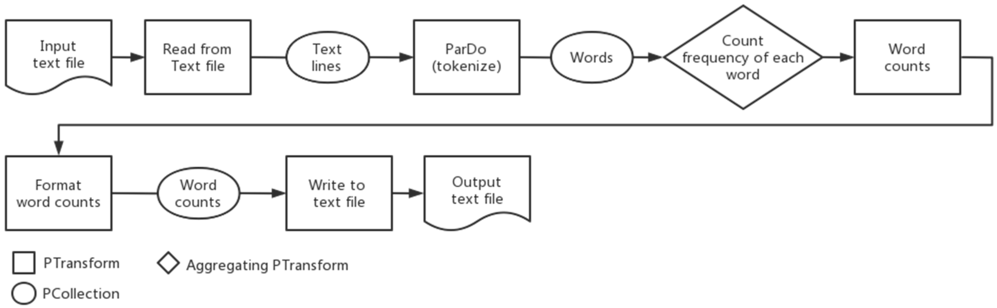
Figure 1. Apache Beam WordCount pipeline data flow.
Information 13 00119 g001
Figure 2. Message of particle 3 (fitness function, sphere function; dimension, 2).
Information 13 00119 g002
Figure 3. Running time and swarm population.
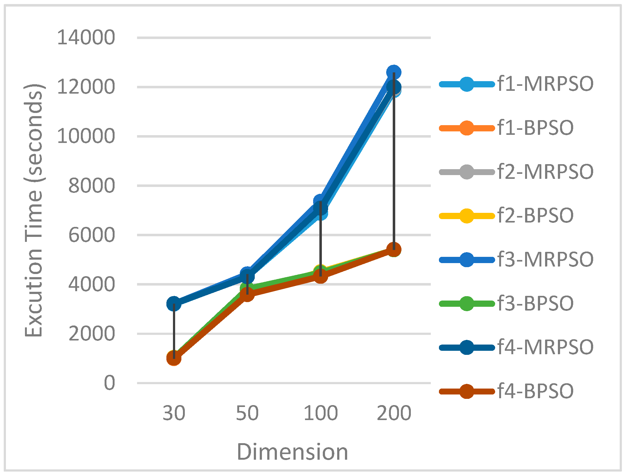
Information 13 00119 g003
Figure 4. Running time and dimensions.
Information 13 00119 g004
Table 1. Benchmark function.
EquationNameBounds
f 1 = i = 1 D x i 2 Sphere/Parabola ( 100 , 100 ) D
f 2 = 1 4000 i = 1 D x i 2 i = 1 D cos ( x i / i ) + 1 Generalized Griewank ( 600 , 600 ) D
f 3 = i = 1 D [ x i 2 10 cos ( 2 π x i ) + 10 ] Generalized Rastrigin ( 10 , 10 ) D
f 4 = i = 1 D 1 [ 100 ( x i + 1 x i 2 ) 2 + ( x i 1 ) 2 ] Rosenbrock function ( 10 , 10 ) D
Table 2. MRPSO and BPSO running time and speedup on f 1 .
NMRPSO TimeBPSO TimeSpeedup
1001198.49436.082.75
5001192.87578.182.06
10002189.19740.492.96
20003197.82988.383.24
Table 3. MRPSO and BPSO running time and speedup on f 2 .
NMRPSO TimeBPSO TimeSpeedup
1001206.55438.462.75
5001213.93637.241.90
10002212.14776.572.85
20003209.241031.513.11
Table 4. MRPSO and BPSO running time and speedup on f 3 .
NMRPSO TimeBPSO TimeSpeedup
1001210.64446.732.71
5001209.00616.241.96
10002209.92770.612.87
20003210.921013.853.17
Table 5. MRPSO and BPSO running time and speedup on f 4 .
NMRPSO TimeBPSO TimeSpeedup
1001203.08450.842.67
5001209.39620.171.95
10002208.28769.742.87
20003215.171008.693.19
Table 6. Mean of the particle best-fit values in MRPSO and BPSO on f 1 . The bold numbers refers to the better results.
NMRPSO Fitness ValueBPSO Fitness Value
100128.14133.96
5009.372.46
10007.090.68
20005.600.41
Table 7. Mean of the particle best-fit values in MRPSO and BPSO on f 2 . The bold numbers refers to the better results.
NMRPSO Fitness ValueBPSO Fitness Value
1002.482.92
5001.091.02
10001.051.00
20001.051.00
Table 8. Mean of the particle best-fit values in MRPSO and BPSO on f 3 . The bold numbers refers to the better results.
NMRPSO Fitness ValueBPSO Fitness Value
10092.7996.45
50093.1643.86
100056.4035.90
200060.6721.58
Table 9. Mean of the particle best-fit values in MRPSO and BPSO on f 4 . The bold numbers refers to the better results.
NMRPSO Fitness ValueBPSO Fitness Value
100208.13214.30
50042.3032.92
100040.4829.94
200037.6727.43
Table 10. MRPSO and BPSO running time and speedup on f 1 .
DMRPSO TimeBPSO TimeSpeedup
303197.82988.383.24
504327.673760.291.15
1006877.074462.221.54
20011,858.535398.022.20
Table 11. MRPSO and BPSO running time and speedup on f 2 .
DMRPSO TimeBPSO TimeSpeedup
303209.241031.513.11
504399.533641.001.21
1007155.964508.831.59
20011,937.035395.532.21
Table 12. MRPSO and BPSO running time and speedup on f 3 .
DMRPSO TimeBPSO TimeSpeedup
303210.921013.853.17
504414.913819.421.16
1007360.374470.321.65
20012,593.525396.432.33
Table 13. MRPSO and BPSO running time and speedup on f 4 .
DMRPSO TimeBPSO TimeSpeedup
303215.171008.693.19
504309.393582.941.20
1007086.784323.711.64
20011,995.855412.742.22
Table 14. Mean of the particle best-fit values in MRPSO and BPSO on f 1 . The bold numbers refers to the better results.
DMRPSO Fitness ValueBPSO Fitness Value
305.600.41
5049.4719.62
100345.25226.72
2001184.811065.62
Table 15. Mean of the particle best-fit values in MRPSO and BPSO on f 2 . The bold numbers refers to the better results.
DMRPSO Fitness ValueBPSO Fitness Value
301.051.00
501.501.19
1004.343.30
20011.9310.37
Table 16. Mean of the particle best-fit values in MRPSO and BPSO on f 3 . The bold numbers refers to the better results.
DMRPSO Fitness ValueBPSO Fitness Value
3092.7921.58
50135.50101.66
100456.46332.56
200948.23909.30
Table 17. Mean of the particle best-fit values in MRPSO and BPSO on f 4 . The bold numbers refers to the better results.
DMRPSO Fitness ValueBPSO Fitness Value
3037.6727.43
50134.1090.79
100505.26400.99
2001438.011291.71
Publisher’s Note: MDPI stays neutral with regard to jurisdictional claims in published maps and institutional affiliations.

