Article

Neural Vocoding for Singing and Speaking Voices with the Multi-Band Excited WaveNet

Analysis/Synthesis Team—UMR 9912 STMS, IRCAM (the Institute for Research and Coordination in Acoustics/Music), CNRS (Centre National de la Recherche Scientifique), Sorbonne Université, 75004 Paris, France
*
Author to whom correspondence should be addressed.
Information 2022, 13(3), 103; https://doi.org/10.3390/info13030103
Submission received: 31 December 2021 / Revised: 8 February 2022 / Accepted: 16 February 2022 / Published: 23 February 2022
(This article belongs to the Special Issue Signal Processing Based on Convolutional Neural Network)

Abstract

:
The use of the mel spectrogram as a signal parameterization for voice generation is quite recent and linked to the development of neural vocoders. These are deep neural networks that allow reconstructing high-quality speech from a given mel spectrogram. While initially developed for speech synthesis, now neural vocoders have also been studied in the context of voice attribute manipulation, opening new means for voice processing in audio production. However, to be able to apply neural vocoders in real-world applications, two problems need to be addressed: (1) To support use in professional audio workstations, the computational complexity should be small, (2) the vocoder needs to support a large variety of speakers, differences in voice qualities, and a wide range of intensities potentially encountered during audio production. In this context, the present study will provide a detailed description of the Multi-band Excited WaveNet, a fully convolutional neural vocoder built around signal processing blocks. It will evaluate the performance of the vocoder when trained on a variety of multi-speaker and multi-singer databases, including an experimental evaluation of the neural vocoder trained on speech and singing voices. Addressing the problem of intensity variation, the study will introduce a new adaptive signal normalization scheme that allows for robust compensation for dynamic and static gain variations. Evaluations are performed using objective measures and a number of perceptual tests including different neural vocoder algorithms known from the literature. The results confirm that the proposed vocoder compares favorably to the state-of-the-art in its capacity to generalize to unseen voices and voice qualities. The remaining challenges will be discussed.

1. Introduction

A Vocoder is a parametric model of speech or singing voice signals that allows reproduction of a speech signal from parameters following an analysis/synthesis procedure. In the case of voice synthesis, the analysis procedure may be replaced by means of a generator that directly produces the vocoder parameters for synthesis. Research into vocoders has a long history. While initial systems were built using electrical circuits [1], most of the known vocoders were implemented in software. Early implementations were the phase vocoder [2], sinusoidal models [3], and pitch-synchronous overlap-add (PSOLA) [4]. Later, a large number of vocoders employing various techniques have been proposed [5,6,7,8,9,10,11]. Most of these systems rely, in one form or another, on the source-filter model of voice production [12,13]. While splitting a voice model into source and filter parts simplifies analysis and representation, it comes with the problem that in the physical world source and filter are strongly coupled [14,15]. As a result, a change in pitch will generally be accompanied by changes in glottal pulse form, formant positions, intensity and noise level. While the precise and robust estimation of these parameters was already a challenging research problem, the formulation of voice models that represent the relevant interactions did remain elusive.
Recently, it has been shown that autoregressive deep neural networks (DNN) can be trained to invert mel spectrograms into high-quality speech signals [16]. By means of a perceptual test, the Ref. [16] demonstrated that compared to natural speech, the speech signals generated by means of the DNN are not perceived as significantly different. Because the mel spectrogram is a parametric representation of speech, the DNN inverting the mel spectrogram is denoted as a neural vocoder. The particular autoregressive structure of the DNN used in the Ref. [16] is called the WaveNet.
The very high quality of the synthesis obtained in the Ref. [16] has triggered strong research activities related to neural vocoders. Initial research into neural vocoders did focus on the problem of the high computational costs for training and running the WaveNet, and on the question of the size of the data sets required for training individual speaker models [17,18,19,20,21]. More recent research activities have begun to investigate multi-speaker models [22,23,24]. Initial results have demonstrated that multi-speaker neural vocoders can generalize not only to unseen speakers, but also to unseen languages and expressivity [23]. In this article, we will follow the Ref. [22] in denoting a neural vocoder that supports multiple voices a universal neural vocoder, noting for clarity that such a vocoder is not as universal as an analysis/resynthesis with a short-time Fourier transform. The quest for a truly universal neural vocoder is one of the motivations of the present work.
Producing a neural vocoder that supports multiple—or even arbitrary—voices can be seen as an enabling technology. For synthesis, a universal neural vocoder not only simplifies the creation of new voices, but also allows building TTS systems with front ends containing a speaker identity control [25]. Such speaker control can be used to switch between existing speakers. However, it may also be used to produce speakers with a combination of features that do not exist in the training database. For speech processing, it allows for the development of DNN systems for voice transformation, for example, for speaker identity conversion [26], pitch transformation [27,28], and gender transformation [29]. At IRCAM, for example, we are currently developing technology that aims to reproduce an artificial singing voice spanning three octaves of vocal range, a capability that is attributed to the voice of Farinelli [30]. As soon as voice transformation becomes creative, the mel spectrograms will almost certainly contain features that cannot be observed in a single original voice, and therefore, a universal neural vocoder is required.
A universal neural vocoder would also allow for the development of versatile real-world applications for classical voice transformation, for example, for cinema and music production, where precise control of speech parameters for arbitrary speakers/singers is desired. For film production, precise modification of speech duration may be necessary. For music production, one may need to globally or locally correct or manipulate the pitch in a singing voice recording. In these cases, modifications need to be precise and the content needs to be preserved as much as possible. The changes should be limited to the attribute modifications that are required to keep the signal coherent overall. This kind of precise attribute editing is the subject of active research for image manipulation [31,32,33] but has not received much attention for voice processing.
The large potential of a universal neural vocoder motivated our research presented in the following. In the long term, this work aims to develop a neural vocoder supporting perceptually transparent analysis/resynthesis for arbitrary speakers and arbitrary voice qualities, notably, the spoken and singing voice.

1.1. Related Work

The neural vocoders mentioned so far all rely exclusively on DNN for signal generation. There are no signal processing components integrated into the generator. Another line of research, more inline with the present study, aims to compose DNN with classical signal modeling techniques to avoid having the DNN learn correlations that can be expressed easily using signal models. A prominent example is DDSP, a python package for differentiable digital signal processing [34,35]. The Ref. [34] proposes to implement a classical additive sinusoidal model [36] using the differentiable operators of a deep learning framework as the signal processing back-end and uses a DNN as the front-end to control the parameters of the additive model. The fact that the signal processing operators are differentiable allows training the whole system as an auto-encoder. The model receives control parameters (F0, instrument type, ...) extracted from a given signal that it has to reconstruct by means of choosing the various parameters of the signal model. Interestingly, during inference, the signal parameters obtained from an input signal can be manipulated before being sent to the front-end. Ideally, if the DNN controller was learned with sufficient examples, and if the input parameter combinations remain in realistic ranges, the DNN controller will be able to translate the input parameters into the most appropriate parameters of the signal model. This setup has two benefits: First, it solves the long-standing problem of high-level control of advanced signal processing models, and second, by means of imposing some structure into the DNN training of the model can be done with fewer data. The key problem is to find a structure that is properly adapted to the target domain not limiting the expressivity of the model.
A prominent candidate for structuring a vocoder into signal processing operators and DNN modules is the source-filter model [12,13]. Adding a filter component into a neural vocoder does not in itself imply any limitations for the signals that may be represented by the vocoder. One of the most basic source-filter models—linear predictive coding (LPC) [12]—can be applied to arbitrary input signals. As mentioned above, a fundamental problem of the classical vocoders is the missing interaction between source and filter, other problems are the linearity assumption and various constraints imposed on the source or filter components. In a DDSP type setup these problems can be solved. The DNN based controller can establish interaction and non linearity, and if either source or filter is a DNN, then the model’s expressivity can also be easily adapted to fit the signals. A particular problem that arises with the introduction of source and filter components is gain ambiguity. If no constraints are established, the source and filter can be modified transparently by means of applying a filter to the source and the inverse filter to the filter. This problem needs to be addressed to achieve a robust parameter estimation.
Indeed, there exist numerous studies [19,37,38,39,40] investigating combinations of DNN and signal processing components for training neural speech vocoders. In most cases, a WaveNet [16] acts as source, which is passed through a filter obtained either from the input signal [40] or by means of a separate DNN [39]. The Refs. [37,38] conditioned a WaveNet on classical acoustic features (e.g., F0, Voice/Unvoiced, ...) to generate an excitation signal and make use of an autoregressive (AR) vocal tract filter (VTF) to construct a speech signal. The Ref. [39] uses a mel spectrogram as input and conditions a model resembling the WaveNet on features derived from the mel spectrogram. The VTF is obtained directly from the mel spectrogram by means of straightforward mathematical operations. Most of these systems are using a multi-resolution spectral loss as objective function. A particularity of [39] is the incorporation of an adversarial loss. The Ref. [40] did not use a WaveNet for the excitation generation, but instead relies on WaveGlow [18]. Finally, the Ref. [19] did not use a classical VTF component, but a neural filter module to modify an excitation consisting of the output of a sinusoids-plus-noise model with seven partials. The neural filter module then took care of completing the missing parts of the excitation and creating the formant structure.

1.2. Contributions

In the Ref. [41], we presented our first results concerning the Multi-Band Excited WaveNet (MBExWN), a neural vocoder performing a perceptually nearly transparent analysis/resynthesis for seen and unseen voice identities, as well as seen and unseen voice qualities. In Ref. [41] we were using two different models, one for speech and the other for singing voice. The present paper introduces the following innovations compared to the Ref. [41]:
Automatic and adaptive signal normalization: A universal neural vocoder should work independently from the signal energy. The existing normalization strategies standardize either the full training database, individual speakers, or individual phrases. In all cases, the standardization poses the problem that the maximum amplitude will depend on the distribution of signal amplitudes. Practically, this means that the amplitude of the same content of a signal will depend on the number and length of pauses. Correctly handling these irrelevant amplitude variations will waste resources in the neural vocoder. To address this problem we will introduce a fully adaptive, time-varying signal normalization strategy for neural vocoders conditioned on mel spectrograms that eases the practical use of a neural vocoder in signal processing applications. We discuss our results in an experimental evaluation comparing the adaptive normalization with a more straightforward gain augmentation of the training dataset. To our knowledge, this is the first time the impact of a variation of signal gain has been studied for a neural vocoder working in an analysis/synthesis setup.
Ablation study motivating the MBExWN model topology: [41] does not provide an objective evaluation of the various model components. We provide explicit parameter settings for the pseudo quadrature mirror filterbank (PQMF) and evaluate a few model configurations in form of an ablation study. The results support the effectiveness of the model structure proposed in the Ref. [41].
Investigation of model deficiencies: [41] proposes to use two distinct models for speech and singing voices. This is unfortunate, notably for practical applications. The present study will investigate the performance of the MBExWN model when trained on both singing and speaking voices. Furthermore, the Ref. [41] found that the synthesis of rough voices does not work well. The present study confirms this result and provides some theoretical insights into their origin.
The rest of the paper is organized as follows. In Section 2.1 we will describe and motivate the model topology, in Section 2.2 we will discuss the loss functions that are used for training, in Section 2.3 we will introduce the signal adaptive normalization strategy, and in Section 3 will describe the data sets and discuss our experimental results. In Section 4 we will discuss our findings and put them into perspective.

2. Materials and Methods
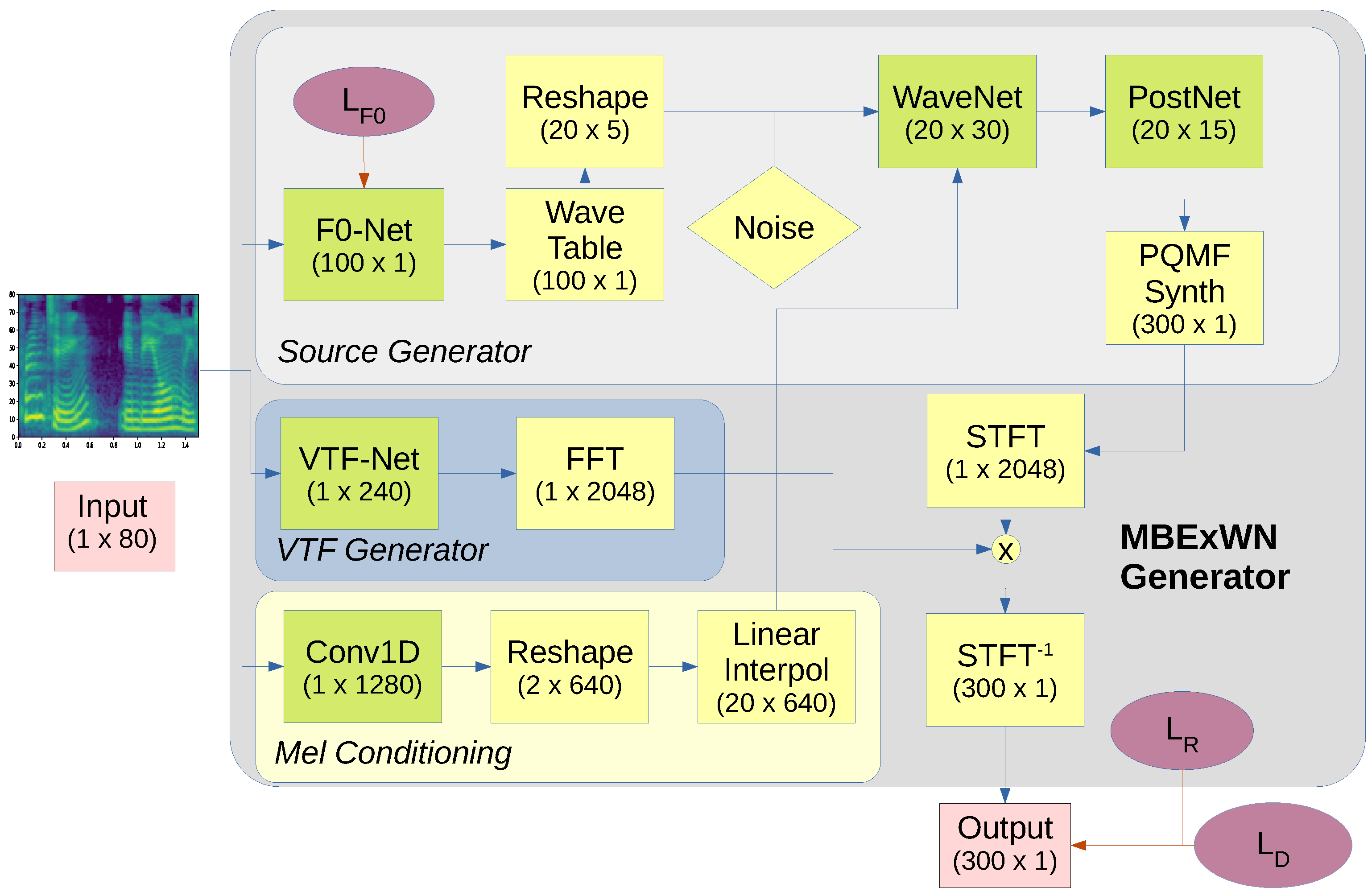
As an introduction into the following analysis, we present the MBExWN model, which due to space constraint, was introduced rather briefly in the Ref. [41]. The overall structure of the neural vocoder is shown in Figure 1. All green blocks are DNN submodules and yellow blocks represent signal processing operators. Red ovals represent loss functions which will be described in Section 2.2. Please note that for the experiments discussed in the following the input mel frame rate of the vocoder is 80 Hz, and the vocoder generates an output sample rate of 24 kHz.

2.1. Model Topology

For constructing the various submodules of the MBExWN generator, we use three variants of convolutional layers together with a few activation functions and the reshape operator. The convolutional layers to be used will be denoted as follows:
Conv1D: 
The classic one-dimensional convolutional layer.
Conv1D-UP: 
A Conv1D layer followed by a reshape operator. Conv1D-UP is used to perform upsampling using sub-pixel convolution and is initialized with checkerboard free initialization following [42].
LinConv1D-UP: 
A Conv1D-Up layer with fixed, pre-computed weights followed by a reshape operation. The weights are pre-computed such that the layer performs upsampling by means of linear interpolation.
Note that the Conv1D and Conv1D-UP layers use weight normalization according to the Ref. [43]. The model uses the following three activation functions: leaky ReLU with the slope for the negative part of the input set to 0.2, fast sigmoid defined as
y = 0.5 + 0.5 x 1 + | x | ,
and finally, for the WaveNet, gated activations as proposed in the Ref. [44]. As a motivation for using fast sigmoids we note that we do not expect the network to require the hard saturation provided by a standard sigmoid function, and therefore selected the fast variant for its lower computational complexity.

2.1.1. VTF Generation

In line with the discussion from the Ref. [37], we decided to use an STFT-based VTF module such that the internal vocoder only needs to produce an excitation signal, and does not need to deal with the rather narrow vocal tract resonances. The VTF network translates the input mel spectrogram into 240 causal cepstral filter coefficients. These coefficients are then converted into a spectral envelope by means of applying a DFT. Note that the use of causal cepstral coefficients implies that the resulting filter is minimum phase [45]. Furthermore, the limitation of the number of cepstral coefficients provides efficient control over the minimum formant bandwidth [46], which allows for avoiding extreme resonances that may arise with autoregressive filters in case that a pole comes too close to the unit circle. The VTF network is very simple as it does not need to perform any upsampling. The details of the VTF-Net are shown in Table A1 in Appendix A.1.
The output of the VTF-Net needs to be converted further into a complex STFT so that it can be used for spectral domain filtering. This conversion is not straightforward due to two problems: First, the gain ambiguity that was mentioned in the introduction, and second, the limited range of the representation of the floating point variables that may lead to NaN notably for the gradient calculation of the VTF. To solve these two problems we constrain the filter to a limited range in dB and normalize the energy of the final filter transfer function to force the filter to preserve frame energy. Accordingly, for each frame m the causal cepstral coefficients c m , k are converted into a complex spectrum S m as follows:
L m = RFFT c m , k
S m = exp r max tanh Re ( L m )   +   i Im L m
S m = N · S m | S m | 2       for m = 0 , 1 , ,
where RFFT is the FFT of a real-valued signal (discarding the negative frequency axis, due to symmetry), r max is a the maximum filter gain or attenuation, Re and Im are the real- and imaginary parts respectively, and N is the number of frequency bands. For all models discussed in the following, we have r max = 40 dB.
The application of the VTF by means of spectral-domain filtering requires a specification of the STFT window and FFT size for the STFT blocks in Figure 1. To allow an appropriate representation of the formant structure the STFT window needs to be longer than the filter impulse response of the formants. Using fundamental relations between bandwidth and decay rate for individual poles [47], one can conclude that a Hanning window of 50 ms should allow for a reasonable approximation of formants with bandwidths above 40 Hz. We note that according to the Ref. [46] a cepstral filter with 240 coefficients achieves a frequency resolution of about 50 Hz. If a better VFT precision is desired the STFT window should be increased together with the number of cepstral coefficients.

2.1.2. Excitation Generation

A crucial element of a neural vocoder is the generation of the quasi-periodic excitation. In our own initial investigations, we found that notably for the singing voice, the existing approaches like multi-band MelGAN [21] and WaveGlow [18] had problems generating long stable pitch contours for the voiced segments. Therefore, similar to the Ref. [19], we decided to generate a periodic excitation. However, because the F0 is not used as input feature, we needed to generate the F0 contour from the mel spectrogram. For this we used the F0-Net in Figure 1. The F0-Net is a rather straightforward multi-layer CNN with a topology specified in Table A2 in Appendix A.2.
The F0-Net has an upsampling factor of 100, which means that for a 80 Hz mel frame rate the F0 sequence is generated with a sample rate of 8000 Hz. For the next stage, we need to convert the F0 into a quasi-periodic excitation. In a first step, we will translate the output of the F0-Net, denoted as y n , into a phase contour. This is achieved as follows:
F 0 n = F 0 m i n + ( F 0 m a x F 0 m i n ) y n
ϕ n = ( k = 0 n F 0 k / R ) mod 1 ,
where F 0 m i n and F 0 m a x denote the minimal and maximal f0 we want to be able to generate, and R denotes the sample rate. In the following experiments we use F 0 m i n = 45 Hz and F 0 m a x = 1400 Hz. The result ϕ n is a normalized phase that can be used as an index into a wavetable or as an argument for a trigonometric function.
For transforming the phase function into an excitation signal, the Ref. [19] proposed to use a sinusoidal model with seven harmonics. Unfortunately, for very high-pitch singing (note that for specific productions we are currently working on our training database containing soprano singers’ singing with F 0 = 1400 Hz), the upper sinusoids will produce aliasing. To avoid aliasing, we have experimented with two approaches. The first is a sinusoidal model containing only one harmonic given by:
e n = 0.5 sin ( 2 π ϕ n ) ( 1 cos ( 2 π ϕ n ) ) ,
where ϕ n is the phase contour described above. This excitation signal is always band limited to 2F0 and therefore does not produce aliasing in our setup. The second approach is using a set of 13 wavetables with a properly selected number of harmonics such that band-limited synthesis can be performed for a limited F0 range. Notably, the upper F0 in Hz for each wavetable is given by
W i = 125 × 1 . 25 i .
Thus, the first wavetable will be used for F 0 < 125 Hz and contains 30 harmonics, where the last one for F 0 > 1800 Hz contains only two harmonics. For intermediate F 0 , we sample with a weighted sum of the two closest wavetables. The two excitation generators will be compared in the ablation study in Section 3.2.3.
The output of the wavetable operator is then reduced in sample rate by means of time to channel folding with factor 5 and concatenated with a white noise signal. This intermediate signal therefore has a sample rate of only 1600 Hz, which allows to operate the pulse-forming WaveNet efficiently. The WaveNet is conditioned on the mel spectrogram that is upsampled to match the internal sample rate of 1600 Hz. As the WaveNet does not need to produce any oscillation, we can greatly reduce its computational complexity and run it without recursion. We use two WaveNet blocks with five layers each. The WaveNet is run with padding SAME, kernel size 3, and a dilation factor that increases by factor 2 with each layer. The number of channels of the WaveNet blocks will be denoted C W in the following. Our default setup is C W = 320 , but for the model that represents singing and spoken voices, we use C W = 340 . The last layer of each WaveNet block uses a Conv1D layer with filter size 1 and 30 channels. With this configuration, each WaveNet block has a receptive field of 41 ms. Note that in the present setup, each WaveNet block is designed to have a receptive field that covers about two periods of the lowest F0 supported by the model. Given the WaveNet only acts as a pulse former and not as an oscillator, longer receptive fields are not required. The output of the second WaveNet is then fed into a PostNet with a single Conv1D layer with filter size 1 that produces a 15-channel version of the excitation signal with 1.6 kHz.

2.1.3. The PQMF Synthesis Filter

The final stage performs the upsampling of the 1.6 kHz PostNet output with 15 channels to the final rate of 24 kHz. Here, we have experimented with two options; notably, the sub-pixel convolution that is also used for the F0 prediction, and a PQMF synthesis filter.
The use of a PQMF synthesis filter as an upsampling operator within a DNN was proposed in the Ref. [48] with a four-band PQMF. The same PQMF was later used in the Ref. [21] for the multi-band MelGAN. The general argument is that the PQMF synthesis filter allows generating channels with considerably reduced redundancy, leading to a reduction in computational complexity. As will be shown in the experimental evaluation in Section 3.2.3, the PQMF approach indeed leads to a slightly lower reconstruction error. In our setup, we need a 15-band PQMF synthesis filter that we have designed using the procedure described in the Ref. [49] using the Kaiser window with shape parameter β = 9 . This allows achieving a stopband attenuation of approximately 90 dB. We selected a filter with 120 coefficients and pass-band transition starting at 0.042 π . The filter transfer function is displayed in Figure 2. The limitation to 120 coefficients does not allow a very steep transition, but the stopband suppression with 90 dB effectively suppresses any cross-talk over more than two neighboring bands.

2.2. Loss Functions

As objective functions, we use the following loss functions. The first loss is the F0 prediction loss given by
L F 0 = ( k K | F k F ^ k | ) / k 1 .
F k is the target F0 and F ^ k are the predicted value at time sample position k K , and K is the set of points that are voiced and sufficiently far away from any voiced/unvoiced boundary such that we can assume the ground truth F0 is correct. In the present study, we used points k that are annotated as voiced and further than 50 ms away from a voiced/unvoiced boundary. For these unambiguously voiced sections, the F0 predictor can be optimized using only the prediction error.
The second loss is a multi-resolution spectral reconstruction loss similar to the Ref. [23]. It is composed of two terms—the first one is calculated as normalized RMSE magnitude differences, and the second as log amplitude differences.
L A   =   S S ^ F / S F , and
L L = 1 K M log ( S ) log ( S ^ ) 1 .
Here, S and S ^ are the magnitudes of the STFT of the target and generated signals, K, and M are the number of frames and the number of bins in S, and . 1 and . F are the L1 and Frobenius norm, respectively.
The final reconstruction loss is then the mean of the reconstruction losses obtained for the different resolutions
L R = ( j ( L A , j + L L , j ) ) / j 1 ,
where j runs over the resolutions. For the following experiments, we used STFT with window sizes 15 ms, 37.5 ms, 75 ms and hop sizes 3.125 ms, 7.5 ms, 15 ms. The reconstruction loss is used as an objective function for the pulse shaping WaveNet and the VTF-Net.
Finally, when training with the discriminator loss L D , we use nearly the same discriminator configuration and loss as the Ref. [23]. The only difference is that instead of using three discriminator rates, we only use two. The first one works on the original sample rate, and the second on a reduced sample rate obtained by means of average pooling of factor 4. We motivate the decision to drop the last discriminator with the fact that the stability of the periodic oscillations is already ensured by the excitation model and therefore the discriminator is only needed to evaluate the pulse form and the balance between deterministic and stochastic signal components.

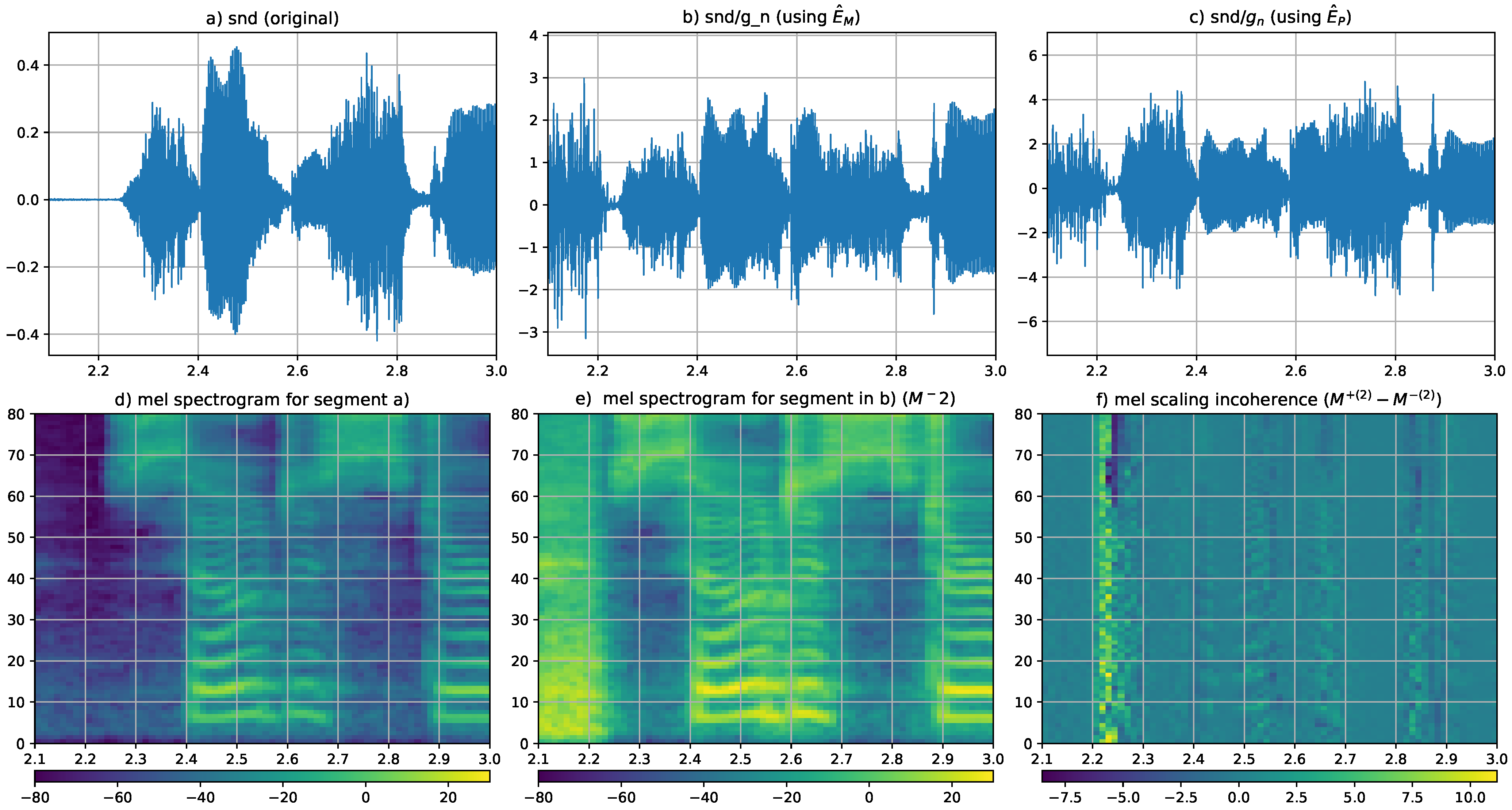
2.3. Signal Adaptive Data Normalization

Due to the internal nonlinearities, a neural network is sensitive to data scaling. Therefore, for any real-world application, proper scaling of the input data needs to be ensured. The problem is not straightforward to solve for a neural vocoder that should work for voice processing in a digital audio workstation. Data standardization [50], which means that the input data is standardized, is no solution because the standard deviation of an audio signal strongly depends on the presence of pauses. In the following, we will investigate two other solutions. The first is based on data augmentation. In this case, training will be performed on data sets with a random constant gain applied to the audio files. After training, the network should be able to handle mel spectra in an amplitude range that was covered by the augmented data set. The problem with this approach might be that training with augmented data will bind network resources such that performance degrades. The second solution is based on a new, adaptive signal normalization that tries to ensure that any given signal content always appears to the network with the same level. This is achieved by means of a pair of gains—the first being applied to the mel spectrogram, and the second, compensating the first is applied as a gain contour on the synthesized signal. In the following, we will introduce the proposed adaptive signal normalization scheme. The experimental evaluation of both strategies will be performed in Section 3. The proposed adaptive normalization proceeds in four steps:
  • Derive an appropriate pair of gain sequences ( G l , g n ) from the sequence of log amplitude mel spectra, M l .
  • Shift the log amplitude mel spectrum M l by means of − log G l .
  • Apply the neural vocoder on the normalized mel spectrogram; and
  • Multiply the generated signal by means of g n .
In the above list and in the following discussion, the subscript l indicates the frame index of a mel- or STFT spectrogram, and the subscript n indicates the sample index of a time signal. Ideally, the pair ( G l , g n ) is selected such that for arbitrary signals x n with mel spectrogram frames M l , the signal x n g n has a mel spectrogram with frames M l + log G l . Accordingly, the selection of an appropriate pair ( G l , g n ) is the key to the normalization strategy.

Estimation of Normalization Gain Contours from the Log Amplitude Mel Spectrogram

We start by acknowledging that there is only one solution that creates perfect coherence between gain changes applied via G l and g n . This ideal solution is G l = g n = c , which means the gain is constant. This solution seems sub-optimal for the normalization problem described above where we want local segments to have approximately constant energy. We therefore search for a sufficiently smooth g n such that the incoherence which is produced as a result of the differences between the scaling operations has a negligible perceptual impact.
Because the signal x n is given to the vocoder only in form of the frames of the mel spectrogram M l , the gain sequences need to be derived from M l . As the initial step, we need to estimate the signal energy that is present in the analysis frame described by a mel spectrum. For this, we make use of Parseval’s theorem, which states
( w a , l h n x n ) 2 = 1 N k N | X l , k | 2 ,
where X l , k is the bin k frame l in the N-point STFT of the frame l of signal x windowed with analysis window w a , n and h the step size between the STFT frames. We denote as X l the vector containing the magnitudes of all bins of frame l. Now the question is: How do we get an estimate of the energy of frame X l given only the log amplitude mel spectrogram M l of the corresponding frame? Clearly, the answer depends on the way the mel spectrogram is calculated. In our study, we used yh python package librosa [51] to generate the mel filter bank B using filters that individually sum to one. Using this filter matrix the mel spectrogram is calculated by means of
M l = log ( | X l | B ) .
This means that M l is a vector containing the average bin amplitude over each mel band for frame l. We tested two approaches to estimate the frame energy. The first uses the pseudo-inverse of the mel filter bank B + and can be written as
X ^ l = max ( exp ( M l ) B + , 0 ) ,
E ^ P , l = 1 N k N | X ^ l , k | 2 ,
and the second directly uses the average amplitudes present in the mel spectrum
E ^ M , l = 1 N k ( 0.5 b k exp ( M l , k ) ) 2 ,
where b k is the number of bins in mel band k and the factor 0.5 is to compensate the fact that the mel band filters overlap so that each bin counts twice in the sum Equation (17). Note that Equation (17) is correct if the energy in each band would be concentrated in the center of the band, which is quite obviously not the case. The value E M therefore overestimates the energy of all bands that contain more than a single bin, and the greater the width of the band, the more this will happen. Interestingly, as will be demonstrated below, this systematic error will not have a negative effect when training with the normalized signals.
Given the energy estimates of the individual frames, we can now calculate the L individual frame scaling factors that will produce signal frames with approximately equal energy. The gain factors are
G l = 1 E ^ M , l .
Note that here, we have used the result from Equation (17) as an example but that the same procedure applies for Equation (16). To find a gain function g n that approximately results in gain changes G l for the signal frames, we employ an iterative smoothing procedure inspired by the Ref. [52]. We denote by ( G l ( i ) , g n ( i ) ) the state of the pair of gain sequences at iteration i and set G l ( 0 ) = G l as a start value. From G l ( i ) , we produce a smoothed gain function by means of overlap, adding a gain synthesis window w s that has a length of α times the length of the mel spectrum analysis window and that are scaled with the G l ( i ) as follows
g n ( i ) = l G l ( i ) w s , l h n .
From this g n ( i ) , we can produce a new G l ( i + 1 ) by means of windowing with the analysis window w a , n
G n ( i + 1 ) = n g n ( i ) w a , l h n .
With increasing i, the differences between neighboring frames will decrease, and the coherence between the gain changes applied in the time and the spectral domain will increase. We can measure the incoherence using the difference
D l ( i ) = M l + ( i ) M l ( i )
δ ( i ) = 1 L N l L | D l ( i ) |
Δ ( i ) = max l , k | D l , k ( i ) | ,
where M l + ( i ) is the mel frame after subtracting log ( G l ( i ) ) , and M l ( i ) is the mel spectrogram computed from the normalized signal x n / g n ( i ) . As an example, we use the signal segment shown in Figure 3a. The mean and absolute error values according to Equations (22) and (23) for an the STFT analysis with w a , n a Hanning window of length 50 ms, a hop size of h = 12.5 ms, and a mel analysis with 80 bands distributed between 0 and 8 kHz and α = 2 are shown in Table 1. As expected, we observe that the maximum and mean error decreases with the number of smoothing iterations that is performed. The average error is rather small already after one iteration. On the other hand, the maximum error in dB remains quite large.
For a further study of the effect and the inconsistency, we refer to Figure 3. The first row displays the effect of the normalization using the two different energy estimates, that is, Equations (16) and (17). A short segment of a speech signal is shown in Figure 3a. The same segment after applying the smoothed time-domain gain g n ( 2 ) obtained with the two different energy estimation methods are displayed in Figure 3b,c. Figure 3b displays the result obtained by estimating the energy without applying the pseudo inverse. Comparison of images Figure 3b,c reveals as expected that the energy estimate E ^ M is systematically too high, and therefore the normalized signal ends up with a smaller amplitude compared to Figure 3c. More interesting is the comparison of the normalization in the unvoiced and voiced segments that can be clearly distinguished in the mel spectrogram in Figure 3d. Notably, the fricatives are located around 2.3 s and 2.8 s. While the stronger over-estimation of the energy in the higher mel bands leads to the fricatives in Figure 3b to be smaller in amplitude compared to the voiced segments (2.5 s), the gain function computed from the spectrogram obtained by means of the pseudo-inverse produces higher amplitudes for the fricatives than for the voiced segments. The image Figure 3e displays the mel spectrogram M ( 2 ) of the normalized segment shown in Figure 3b. One can clearly note an overall shift to higher amplitude levels. Finally, the visualization of the time-frequency distribution of the difference calculated in Equation (21) are shown in image Figure 3f. The largest differences are concentrated in the part where the signal transitions into silence. This is reassuring because it means that the perceptual effect of the relatively large incoherence in that segment remains limited.

3. Results

The following experiments use the same four databases and a similar experimental design as the Ref. [41]. However, the focus of the perceptual evaluation has changed. While in the Ref. [41] the objective was to compare multi-speaker and multi-singer MBExWN models to models trained on individual speakers and singers, here the focus is comparing the multi-speaker and multi-singer models to a single multi-voice model trained on speech and singing databases. Compared to the Ref. [41] the changes in the following evaluation are the following:
  • An objective evaluation of the adaptive normalization strategy has been added.
  • Training the vocoder with random gain augmentation has been added as an alternative strategy to avoid problems with gain variations during inference.
  • A new voice model trained jointly on singing and speech database has been added to study the effect of increasing diversity in the training set.
  • To not overcharge the perceptual tests the single singer and single speaker MBExWN models are no longer used in the test.
  • Training parameters have been changed slightly to use smaller and longer batches.
  • Two bugs in the implementation of the reconstruction loss have been fixed, and the set of resolutions used for the reconstruction loss has been adapted slightly.
For all optimizations, we use the Adam optimizer [53] with learning rate l r = 1 × 10 4 . The decay rate parameters are β 1 = 0.9 and β 2 = 0.999 , for training without discriminator and β 1 = 0.5 and β 2 = 0.5 for training with discriminator. Batch size is always 20, and the segment length is approximately 400 ms.

3.1. Databases and Annotations

There are four databases used for training. The first is the LJSpeech single speaker dataset [54] denoted as LJ in the following. The second denoted as SP, is a multi-speaker dataset composed of the VCTK [55], PTDB [56], and AttHack [57] data sets. The SP data set contains approximately 45 h of speech recorded from 150 speakers. For singing voice experiments we used a single singer data set containing a Greek byzantine singer [58] denoted as DI and for the multi-singer model a database composed of the NUS [59], SVDB [60], PJS [61], JVS, [62] and Tohoku [63] data sets, as well as an internal data set composed of 2 pop, and 6 classical singers. This data set contains about 27 h of singing recordings from 136 singers. The last data set will be denoted as SI. A final data set used for training is constructed by means of joining the SI and SP data sets to form what will be denoted as the voice data set VO. The VO data set will be used to study the effect of joining speech and singing data in a single model. For evaluation purposes we use further audio samples that were collected from various sources. Further details will be given in the text.
For completeness, we mention the LibriTTS data set [64] that has been used to train the baseline Universal Mel GAN model that is used in the perceptual evaluation. The LibriTTS data set will be denoted as LT. We stress that we did not use the LT data set for training our own models.
All samples in the data sets were resampled to 24 kHz. All voice files were annotated automatically with F0 contours using the FCN estimator [65] set-up to use an analysis hop size of 2 ms. The F0 contours were then extended to include voiced/unvoiced information. To obtain the voiced/unvoiced segmentation we employ the confidence value C F C N that is output by the FCN estimator together with a harmonicity estimate calculated by IRCAM’s SuperVP software [66] to calculate a harmonicity value H F 0 for the given F0. For all F0 values existing in the annotation, we set the voiced/unvoiced flag to unvoiced whenever min ( H F 0 , C F C N ) < 0.5 . While the harmonicity estimation in SuperVP is not available as an isolated piece of software, it performs similarly to the noise separation algorithm described in the Ref. [67] that separates deterministic and noise components and then calculates H F 0 as the noise/total energy balance over four periods of the F0.

3.2. Evaluation

The following section will compare different variants of the MBExWN model using first objective measures and later subjective tests.

3.2.1. Training

For each model, we first pre-train the F0 prediction model over 100 k batches using only the Equation (9) as objective function. As a next step, we pre-train the full generator without discriminator loss for 200 k batches with the pre-trained F0 model loaded. Fine-tuning of the pre-trained models is then performed in two configurations. For evaluation purposes, we reload the pre-trained models and train generators for 600 k more batches without using adversarial loss. The full models are also initialized from the pre-trained generators and are fine-tuned with the additional adversarial loss for 800 k batches.
The models that are evaluated will be denoted using a code structured like: T-D-C. Here, T is a placeholder for the model type using the following shortcuts: MW: The Multi-band Excited WaveNet introduced here, MMG: the multi-band MelGAN from the Ref. [21], UMG universal MelGAN vocoder from the Ref. [23]. D will be replaced by the data set that was used for training using two symbol sequences introduced above in Section 3.1. The letter C is a placeholder for the way the model was trained. We will distinguish PR for pre-training with prediction and reconstruction error, as well as FD for fine tuning with discriminator loss and FR for fine tuning with only F0 prediction error and reconstruction error.

3.2.2. Evaluation of the Adaptive Normalization Strategy

We start the study with an objective evaluation of the adaptive signal normalization presented in Section 2.3. We will compare the result obtained using the adaptive signal normalization with a simpler approach consisting of training the MBExWN models with different degrees of gain augmentation. The objective of this study is to find the optimal configuration for training the models that will be used in the subsequent perceptive test. This evaluation will be run with five different random initializations of the network weights to assess of the variability of the results. To avoid an excessive amount of training time we limit the evaluation for this case to model configurations MW-SP-PR and MW-SI-PR. The evaluation uses a total of 315 phrases of dedicated test data collected from both training data sets. That means the test data contains speakers that were used during training, but the phrases used for validation have not been used for training. The evaluation is performed with with signals multiplied by gain factors taken from the list S = [ 1 , 0.5 , 0.1 , 0.01 ] . These gain variations are meant to evaluate the robustness of the model against gain changes.
We have compared 16 different normalization strategies with varying smoothing window size (parameter α ), the number of smoothing iterations and the initial energy estimate (Equations (17) or (16)). With respect to gain augmentation we train three different models with gain values randomly drawn from intervals R a = [ γ , 1 ] . The three models are using γ = 0.5 , γ = 0.1 , and γ = 0.01 , respectively. Finally a model trained with γ = 1 constitutes the baseline, which is not taking care of the problem. As a performance indicator we will use the mean absolute difference of the log amplitude mel spectrograms of the input M, and the resynthesized sound M ^ computed as follows:
V j , l , k = max ( M j , l , k , T )
V ^ j , l , k = max ( M ^ j , l , k , T )
R M = 1 J j 1 L j · K l , k | V j , l , k V ^ j , l , k | .
Here, j, l, and k are the file index, frame index, and mel bin index respectively, and J, L j , and K are the number of files used for evaluation, the number of frames for file j, and the number of bins in the mel spectrograms, respectively. We note that we do not claim that this performance measure reflects the perceptual performance of the various configurations. On the other hand, it will provide insight into the impact of the gain changes on the model’s performance given different choices. We prefer evaluating the reconstruction error on the mel spectrogram instead of the STFT because the mel frequency scale appears to be perceptually more relevant than the linear frequency scale that puts too much weight on the frequency bands that are perceptually less important. The lower bound T allows avoiding a strong impact of the perceptually irrelevant small values that may arise in the noise sections. For the present evaluation T = log ( 10 5 ) . Besides Equation (26) we also calculate the F0 prediction error using Equation (9) which will provide another point of view on the way the MBExWN model reacts to gain changes.
We will not show the results of all the configurations here, but refer to Table A3 and Table A4 in Appendix B. We will describe a conclusion of the results in the following.
Considering the mel reconstruction error in Table A3, a first observation is that there are two clearly separated outliers. The models using adaptive signal normalization without smoothing obtain a mel reconstruction error R M > 8 dB. They clearly do not work. In the second group, when ordered according to Equation (26), three different variants are grouped together. The best performance is observed for the models using adaptive normalization with smoothing based on the simplified energy estimator given by Equation (17). The second group is constituted by the models using adaptive normalization with smoothing based on the energy estimator using the pseudo inverse given by Equation (16). The worst performance is achieved by models trained with random gain augmentation. Within the two groups with adaptive normalization, a general trend is that smoothing with the longest smoothing windows performs worse. Overall the degradation due to gain mismatch in the mel reconstruction error remains quite small. The best model trained with gain augmentation is the model trained with random attenuation in the range R a [ 0.1 , 1 ] . It achieves an average mel reconstruction error of 1.758 dB. On the other hand, the best model trained with adaptive normalization achieves 1.52 dB. Given the confidence intervals are in the order of 0.01 dB the difference is statistically significant. On the other hand, depending n the distribution of these errors the perceptual importance of this small difference may be negligible.
Interestingly, when looking into the F0 estimation error evaluated using Equation (9), we find one of the reasons for the increase of the mel reconstruction error. Again all models using adaptive signal normalization obtain the smallest F0 prediction error. While the F0 prediction error is independent of the gain factors and below 1.7 Hz for all but one configuration using the simple energy model in Equation (17), the best model using random gain augmentation achieves an average F0 error of 2.7 Hz. Moreover, we can see that the models trained with gain augmentation suffer from a strong increase in the F0 prediction error for the smallest gain of 0.01. Here, the best-performing model has an average F0 prediction error of 4 Hz.
The effect of the F0 prediction degradation is visualized in the Figure 4. The figure shows a segment of the original mel spectrogram in Figure 4a and mel spectrograms recreated from resynthesized signals together with the difference of those mel spectrograms compared to the original. The resynthesized mel spectrogram and its difference to the original in Figure 4b,c are related to the model trained with adaptive signal normalization with smoothing window size α = 2 and 1 smoothing iteration.
Figure 4d,e show the same content for the model trained with gain augmentation R a [ 0.1 , 1 ] . To avoid cluttering the images with noise all images are displayed using a lower amplitude bound T = 50 dB. Comparing the mel spectrograms in Figure 4b,d, it is hard to see any differences. Comparing the differences in Figure 4c,e, one can easily detect the effect of an F0 error in Figure 4e around 0.5 s.
The evaluation of the different normalization strategies leads us to conjecture that the normalization based on the simpler energy estimate Equation (17) is a better choice for F0 prediction error and mel spectrogram reconstruction error. Accordingly, we will use Equation (17) in the following. Furthermore, even if larger incoherence remains when smoothing is performed over smaller segments the reconstruction error does not degrade. The model seems to be able to compensate for the incoherence winning on the other hand from a more stable signal representation. Accordingly, smoothing can be performed over a short range of about 2–3 analysis windows. To minimize the computational cost of the normalization operation we select α = 2 and perform mel spectrogram normalization after a single smoothing iteration with G ( 1 ) . The synthesized signal is then re-scaled by means of multiplying with 1 / g n ( 1 ) .

3.2.3. Ablation Study

As a next step, again using networks after the pre-training stage, we perform an ablation study. The objective here is to compare a few variants of the model configuration to determine the effectiveness of the model shown in Figure 1. The different variants are denoted as follows:
Default 
The configuration as displayed in Figure 1 using 13 wavetables as described in Section 2.1.2.
Default-2S 
Default configuration using only two sinusoids as shown in Equation (7) instead of the 13 wavetables. This should validate the use of the wavetable.
WT+PQMF
Default configuration with a PQMF analysis filter replacing the reshape operator after the wavetable.
NO VTF
Default configuration without the VTF Generator using the output of the PQMF synthesis filter as the output signal.
NO PQMF
Default configuration with the PQMF synthesis filter is replaced by a reshape operator.
For each of these variants a MW-VO-PR model has been trained with three different initializations with random weights. The evaluation has then been performed over a total of 315 test files from the SI and SP data sets. The results of the ablation study are shown in Table 2.
Table 2 shows that the configuration adding a PQMF analysis filter after the wavetable leads to a marginal degradation. Further investigation reveals that the PQMF analysis filter at that place is better for the SI model but less good for the SP model. Due to the fact that the PWMF analysis filter is computationally more complex the simpler reshaping operation is used after the wavetable. Building the excitation with two sinusoids instead of the 13 wavetables leads to a slight but significant degradation when evaluated over the VO dataset. Because the computational cost of the use of the 13 wavetables remains negligible compared to the rest of the network, we selected the wavetable-based excitation in our default setup. Concerning the PQMF synthesis filter after the PostNet we find that disabling the PQMF produces on average a consistent increase of the reconstruction error. As can be seen from the confidence interval the increase is clearly significant and therefore the PQMF synthesis filter has been included in the default configuration. Finally, removing the VTF-Net and the STFT filter at the output results in a quite noticeable increase in the reconstruction error. The performance degradation is clearly significant, and therefore, the VTF component is included in the MBExWN default configuration. We note that the rather strong positive effect of the VTF Generator motivates a further investigation into the role of the VTF in the overall system. The detailed inspection presented in Appendix C reveals that the source generated after the PQMF synthesis filter is approximately white. On the other hand, the VTF Generator does not only help with creating the formant structure but also contributes to the harmonic structure. Therefore, in contrast to a classical source filter model, it cannot not be understood only as a representation of a VTF.

3.3. Perceptual Tests

The following section describes the three perceptual tests we have conducted to evaluate the perceived quality of the proposed MBExWN model. In contrast to perceptual tests performed in other studies, and due to the intended use of our model for signal manipulation, our main interest is the perceptually transparent resynthesis of the original voice signal. Therefore, we chose to perform MUSHRA tests containing the reference signal and a group of resynthesized signals that the participants can play as they like. The task given was to concentrate on any differences that might be perceived between the original and the resynthesis and to rate the perceived differences on a scale from 0 to 100 with categories imperceptible (80–100), perceptible, not annoying (60–80), slightly annoying (40–60), annoying (20–40), very annoying/no similarity (0–20). All tests have been performed online using the prolific platform (https://www.prolific.co/, accessed on 28 December 2021).
Using an online platform for perceptual tests comes with an increased risk that individual participants do make random choices. To detect such cases we added a hidden reference to all our MUSHRA tests. The hidden reference is denoted HREF in the tables below. As this signal is identical to the reference the result should be high receiving at least a ranking of 80 on the scale described above. To avoid too much impact from participants selecting random results we remove all experiments where the hidden reference receives a ranking lower than 80. Furthermore, there were submissions with people reporting 0. The online form had a dedicated checkbox for technical problems. Participants were instructed to check this box when the sound did not play properly or did not play at all. Now some of the participants selected between 0–20 without selecting the problem checkbox. Still, as none of the examples can reasonably be qualified to have no similarity at all with the reference, these submissions were discarded as well. The number of discarded submissions will be reported for each test.
The first perceptual test compares the generalized voice model MW-VO-FD, to the dedicated singing or speech models MW-SI-FD and MW-SP-FD. We add the model MW-VO-FR trained without discriminator as a lower quality anchor and as well to measure the effect of the adversarial loss. The evaluations are performed on a subset of the test data of the SI and SP data sets respectively. Note that the MW-VO models work with an increased number of WaveNet channels ( C W = 340 ) compared to the specialized models MW-SI-FD and MW-SP-FD for which we use C W = 320 . For this test, we received a total of 100 submissions, 50 for each of the two data sets. We had to discard five submissions considering the quality criteria described before. The test results are displayed in Table 3. Model results displayed slanted indicate the model had seen the tested voice identities during training. The best-performing model is always marked in bold. The evaluation results shown in Table 3, Table 4 and Table 5, represent the average rating of the model. The standard deviation is shown in parenthesis.
The first column indicates the data source the data is taken from. The second column marked HREF represents the results for the hidden reference. In the next two columns, we find the MBExWN models that were trained on either speech or singing data set, and in the two subsequent columns we find the all-purpose voice models trained either with or without discriminator.
First, it is quite reassuring, even considering that we removed outliers below 80, that participants ranked the hidden reference best with a similarity rating of 96 and 95 for both domains. Reassuring as well is the fact that the model trained without a discriminator is perceived as the least similar to the reference from all four candidates. A little bit unexpected is the fact that the MW-VO-FR model is perceived as less annoying for singing than for speech. This may be due to the fact that the participants are more used to listening to spoken voices than to singing voices. Another explanation may be that the MW-VO-FR model has more problems with fricatives and breathing noises that are less strong in the singing database. Now the interesting aspect of the test is the comparison of the dedicated speech and singing voice models MW-SP-FD and MW-SI-FD to the general-purpose voice model MW-VO-FD. The question here would be whether the use of data from the other domain will improve the model compared to the concurrent that is trained only on the target domain. The answer seems to depend on the domain. While for singing voice re-synthesis the general-purpose voice model performs better than the specialized model, for the speech voice synthesis the opposite is true. This result may be explained as follows. The singing voice databases contain rather clean singing with very few noises, while for the models the voiced/unvoiced transitions with perturbations and rather strong noises are more problematic. Having seen these in the speech database can help the general-purpose voice model to better deal with the few noises that exist in the singing voice evaluation while the other way around the general-purpose model is less prepared to deal with these noises than the specific speech model. Note that this does not mean that we can use the MW-SP-FD model for singing because the singing voices may contain pitches for that no examples exist in the speech training database. On the other hand, the perceptual test performed in Ref. [41] has shown that for singing voice with pitches in the range covered by the speech training data base, the speaking and singing voice models performs quite similar.
In the second and third tests, we evaluate the generalization performance of the three MBExWN models with full fine-tuning MW-VO-FD, MW-SI-FD and MW-SP-FD on unseen voice identities. Note that besides the modifications and bug fixes mentioned above, the MW-SI-FD and MW-SP-FD models are retrained variants of the models that have been tested in the Ref. [41]. The new aspect here is the performance of the multi-voice MW-VO-FD model.
Concerning speech we use as the first baseline a single speaker Multi-band MelGAN [21] that we trained on the LJSpeech data set. For training the model we used an implementation from https://github.com/TensorSpeech/TensorflowTTS (accessed on 18 December 2021). In the following this model will be denoted MMG-LJ-FD. As a second baseline we compare our speaking voice models to the Universal MelGAN [23] trained on a data set containing the LJSpeech data set [54] and the Libri-TTS data set [64]. This model will be denoted UMG-LJ+LT-FD. Note, that due to the very large size of the Universal MelGAN (90 M parameters) we could not retrain this model ourselves. We are grateful to Won Jang for allowing us for the purpose of this evaluation to gather his results from the demo page of the Universal MelGAN (https://kallavinka8045.github.io/icassp2021/#unseen-domains-speaker-emotion-language-1, accessed on 18 December 2021). The results of the second test on speech are displayed in Table 4. There were 140 submissions in total for the evaluation. 18 of these had to be discarded from the evaluation due to the quality constraints mentioned above.
Looking into the individual experiments we find that the single speaker Multi-band MelGAN model trained exclusively on the LJ data set is selected as only marginally better than our multi-speaker model for that the LJ speaker was not part of the training data set. The second row uses again examples from the LJ data set this time taken from the Universal MelGAN demo page. We display this separately to compare with the results of the Universal MelGAN also downloaded from the demo page. Note again that the Universal MelGAN training database contains the LJ speaker together with over 900 other speakers. Therefore the LJ speaker is a known speaker for the UMG-LJ+LT-FD model. This speaker is an unseen speaker for the MW-SP-FD model. Still, the perceptual evaluation ranks the MW-SP-FD model more similar to the reference. Finally, for the out-of-domain examples from the demo website of the Universal MelGAN, the UMG-LJ+LT-FD model performs best. These examples contain languages not seen by any model (Chinese, Japanese, Spanish, and German), an unseen speaker with slightly expressive reading, and other unseen speakers. We note that a more detailed analysis reveals that MW-SP-FD and UMG-LJ+LT-FD perform very similarly for all but the expressive reading examples in the UMG(others) evaluation. Here, UMG-LJ+LT-FD receives a rating of close to 90, while MW-SP-FD receives a ranking of 78 consistent with the results for the other sounds from the UMG web page. This outstanding performance on one of the unseen cases is intriguing. It should be noted that UMG-LJ+LT-FD is trained on the LibriTTS corpus that itself contains audiobook recordings. It may well be that there are similar expressive reading examples in the LibriTTS corpus, which in turn would explain the very good performance of the UMG-LJ+LT-FD model for that case. Finally, concerning the MW-VO-FD model we find again that mixing the singing data into the training database does slightly degrade the performance of the MBExWN model when applied to speech synthesis. As a result, the model performs consistently less well than the model trained only on SP.
The final test concerns the study of the performance on unseen singing voices. Here again, one of the baselines is a single singer multi-band MelGAN [21] that we trained on the Dimitrios data set [58]. The model will be denoted MMG-DI-FD. Further, we evaluate our two MBExWN singing voice models on various unseen singers, singing styles, and voice types that have been extracted from the MUSDB18 data set [68]. With the objective to demonstrate the limitations of the singing models when applied to rough singing voices, we collected a few recordings containing creaky and other irregular singing examples from the internet. All these results are displayed in Table 5. During the test, we collected three times 30 submissions, five of which were discarded due to quality problems.
As before the submissions after cleaning the inconsistent responses shows a high level of similarity for the hidden reference. The test confirms the results we observed already in the first test. The multi-voice MBExWN model trained on speaking and singing voices performs consistently better than the singing-voice model MW-SI-FD. The MW-VO-FD is ranked best in all cases, including for the evaluation with the rough singing voices. This confirms that added spoken voices to the training data can be beneficial even for a model used only for singing synthesis. We note that the evaluation on the Pop data extracted from the MusDB shows some degradation. This can be explained with a rather strong amount of reverberation that remains in these solo singing examples. The models cannot reproduce those which is consistent with a weaker similarity rating. The data set with rough voices is an obvious problem. There are creaky, growl, and metal singing voices including a wide variety of cases with strong subharmonics. A detailed analysis of some of these cases reveals that the octave jumps that are required for the MBExWN model to create an excitation with a fading subharmonic poses a problem that can not be solved by the current model setup. Due to the limitation to an excitation with a single periodicity and a rather short receptive field the model has currently no means to prepare an excitation where the singer produces a soft octave jump by means of fading out the fundamental and all even harmonics. It is very likely that the excitation model needs to be changed to be prepared to handle this kind of excitation. On the other hand, for the moment we do not have a sufficient number of examples to be able to train a modified model to properly handle these cases that exist in various configurations.

3.4. Computational Complexity

The MBExWN models MW-SP-FD and MW-SI-FD have C W = 320 WaveNet channels and about 10M parameters. The model achieves inference rate of 50 kHz when running on a single core of an Intel i7 laptop CPU. For the 24 kHz model, this inference rate corresponds to a generation that is two times faster than real-time. On a NVidia V100 GPU the inference rate is 2.4 kHz, which means on such a high-performance GPU the model is about 100 times faster than real-time. These measures have been obtained using a model that was exported into a configuration that does no longer allow optimization. The sounds used for the test had a duration of at least 20 s of audio. Each sound was processed individually using batch size 1. We note that the MW-VO-FD model has C W = 340 WaveNet channels and about 11 M parameters. For this case, the inference speed decreases by about 10%. The model compares favorably with the Universal MelGAN [23] that has been used in the perceptual evaluation above. The Universal MelGAN has 90M parameters and, according to the Ref. [23], achieves an inference speed of 860 kHz on a V100 NVidia GPU.

4. Discussion

Neural vocoders are an emerging technology opening new perspectives for voice signal processing. The majority of the literature considers the neural vocoders under the perspective of using them for speech synthesis and covers single speaker models vocoders. In contrast to this, the present study investigates neural vocoders from the perspective of general voice processing backends. The mel spectrogram is seen as a low dimensional yet feature-complete representation of voice signals that has the potential to be used as an internal representation for a wide variety of voice attribute manipulation systems. This kind of attribute manipulation with DNN is an established line of research for image processing. We believe that the research activities related to attribute manipulation for images are facilitated by the fact that image manipulation can be performed directly on the images. For voice signals, attribute manipulation is hindered by the fact that reconstruction of a voice signal from an encoding is in itself already a difficult problem. This is due to the fact that the reconstruction loss operating directly on the voice signal does not provide a meaningful loss. Accordingly, the existing voice transformation algorithms are often trained using objectives that require reconstructing mel spectrograms [26,27,28], and in turn, require a solution for the mel inversion problem.
The present paper aims to support these research activities by means of establishing a neural vocoder that allows generating high-quality voice signals from mel spectrogram representations of voice signals covering a wide variety of languages, voice qualities, and speakers or singers. In contrast to all existing research activities, we chose to not evaluate our neural vocoder using a perceptual test using MOS grades but instead performed a MUSHRA test evaluating the degree of transparent reconstruction of the original. This reflects the objective to develop an algorithm that does not only produce high-quality voice signals; instead, the algorithm should reproduce the original voice transparently, such that it can be used to precisely manipulate individual attributes [32].
The present study translates ideas introduced in the DDSP package [34,35] to the problem of neural vocoding. It demonstrates that a multi-voice neural vocoder achieving efficient and near-transparent resynthesis can be constructed by means of appropriately combining classical signal processing components with DNN modules. The signal processing modules are a wavetable, a pseudo-quadrature mirror filterbank, and a cepstrum-based frequency domain VTF generator followed by a spectral domain filter. The vocoder achieves real-time processing using only a single core of a laptop CPU. The perceptual evaluation demonstrates that compared to a state-of-the-art multi-speaker neural vocoder, the Universal MelGAN [23], the proposed multi-speaker model achieves approximately the same performance using 9 times fewer parameters. The model was trained with about 5 times fewer examples and is approximately three times more efficient. This comparison seems to confirm the beneficial impact of the dedicated signal processing blocks.
The study has demonstrated two approaches to create robust performance even when applied to voice signals that vary by about 40 dB in signal intensity. This is achieved by means of an adaptive normalization that remains computationally negligible compared to the rest of the vocoder components. Combining efficiency, high quality, and robustness against intensity changes is an essential step towards integrating neural vocoders into professional audio production software and for manipulation of speaking and singing voice attributes [69].
The study has demonstrated a few deficiencies of the present implementation. Integrating speech and singing voice into a single vocoder improves the results for singing voice but degrades the performance for speech. Here, further research is clearly required. Increasing the number of parameters is a possible option, but would increase computational costs. We are currently investigating architectural changes that hopefully will improve expressivity without increasing computational costs such that the vocoder allows better coverage of voice qualities in the same model. A further problem for the current neural vocoder are rough and saturated voices that are rather important for singing applications, but for that, hardly any signal processing algorithms exist.

Demonstration Material

To facilitate research into voice attribute manipulation using the mel spectrogram as voice representation, the trained models MW-SI-FD, MW-SP-FD, and MW-VO-FD together with a Python/Tensorflow package that allows inference with these models is available online (https://github.com/roebel/MBExWN_Vocoder, accessed on 1 February 2022). The same page provides also access to sound examples from the perceptual tests in Section 3.3.

5. Conclusions

In this paper, we have extended a previous study concerning the Multi-band Excited WaveNet: a neural vocoder containing a wavetable-based generator coupled with a WaveNet as the excitation source. We have proposed a new adaptive signal normalization algorithm that is performed on the fly and improves the robustness of the vocoder against intensity changes of up to 40 dB. A perceptual test has shown that the proposed model achieves near-transparent resynthesis quality even for out-of-domain data. The signal degrades when confronted with rough and saturated voices. Further research will be conducted to solve these cases.

Author Contributions

Conceptualization, A.R. and F.B.; methodology, A.R. and F.B.; software, A.R.; experimental study, A.R. and F.B.; data curation, A.R. and F.B.; writing—original draft preparation, A.R.; writing—review and editing, A.R.; visualization, A.R.; project administration, A.R.; funding acquisition, A.R. All authors have read and agreed to the published version of the manuscript.

Funding

This research was funded by ANR project ARS, grant number ANR-19-CE38-0001-01 and computation were performed using HPC resources from GENCI-IDRIS (Grant 2021-AD011011177R1).

Institutional Review Board Statement

Ethical review and approval were waived for this study, due to the fact that perceptional tests have been performed online using the dedicated web service provided by prolific https://www.prolific.co/ (accessed on 28 December 2021). The service of prolific implies that participants contribute online, fully anonymously, and voluntarily. Moreover it implies that participants are free to choose the studies they want to participate in from a list of online surveys, and that they can opt out at any time.

Informed Consent Statement

Informed consent was obtained from all subjects involved in the study. By means of a text presented during the announcement of the test participants have been informed before the study starts about: the general goals and duration of the online survey; the payment that can be expected when finishing the survey; and the fact that their answers will be used to establish average responses to the questions for a scientific publication on audio quality.

Data Availability Statement

All speech data used for training the models is publicly available by means of the links provided in the document. For singing data, there are about 2 thirds publicly available by means of the links provided in the document and 1 third of the singing data mentioned as internal recordings are owned by IRCAM and cannot be made publicly available.

Acknowledgments

The authors would like to thank Won Jang for sharing information and materials related to the universal MelGAN [23].

Conflicts of Interest

The authors declare no conflict of interest. The funders had no role in the design of the study; in the collection, analyses, or interpretation of data; in the writing of the manuscript, or in the decision to publish the results.

Abbreviations

The following abbreviations are used in this manuscript:
DNNDeep neural network
MBExWNMulti_band Excited WaveNet
PQMFpseudo quadrature mirror filterbank
VTFvocal tract filter

Appendix A. Model Topology

The present section regroups detailed specifications concerning the layers of the VTF-Net and the F0-Net displayed in Figure 1.

Appendix A.1. VTF-Net

Table A1. Layers of the VTF-Net. For layer type notation see Section 2.1.
LayerFilter Size# FiltersActivation
Conv1D3400leaky ReLU
Conv1D1600leaky ReLU
Conv1D1400leaky ReLU
Conv1D1240-

Appendix A.2. F0-Net

Table A2. Layers of the F0-Net. For layer type notation see Section 2.1.
LayerFilter Size# Output FeaturesUp-SamplingActivation
Conv1D3150 leaky ReLU
Conv1D-Up31502leaky ReLU
Conv1D5150 leaky ReLU
Conv1D3120 leaky ReLU
Conv1D-Up31205leaky ReLU
Conv1D1120 leaky ReLU
Conv1D-Up31005leaky ReLU
Conv1D1100 leaky ReLU
Conv1D350 leaky ReLU
LinConv1D-Up 2fast sigmoid

Appendix B. Adaptive Normalization

The tables below contain the mel reconstruction errors Equation (26) and F0 prediction errors Equation (9) discussed in Section 2.3.
Table A3. Mean mel reconstruction errors on for mel spectrograms rescaled by the factor S. All errors in dB with a 95% confidence interval.
NormalizationAverage S = 1 S = 0.5 S = 0.1 S = 0.01
norm_M(3, 1) 1.520 ± 0.007 1.403 ± 0.008 1.410 ± 0.009 1.534 ± 0.012 1.734 ± 0.014
norm_M(2, 1) 1.525 ± 0.007 1.393 ± 0.008 1.410 ± 0.009 1.555 ± 0.012 1.742 ± 0.014
norm_M(3, 3) 1.527 ± 0.007 1.392 ± 0.009 1.406 ± 0.010 1.549 ± 0.013 1.763 ± 0.014
norm_M(1, 3) 1.531 ± 0.006 1.423 ± 0.008 1.433 ± 0.009 1.556 ± 0.012 1.712 ± 0.014
norm_M(1, 2) 1.531 ± 0.007 1.406 ± 0.008 1.421 ± 0.010 1.559 ± 0.013 1.738 ± 0.014
norm_M(1, 1) 1.534 ± 0.007 1.403 ± 0.008 1.421 ± 0.010 1.570 ± 0.013 1.743 ± 0.014
norm_M(2, 2) 1.535 ± 0.007 1.411 ± 0.008 1.423 ± 0.010 1.559 ± 0.013 1.747 ± 0.014
norm_M(10, 3) 1.556 ± 0.007 1.430 ± 0.009 1.438 ± 0.011 1.559 ± 0.013 1.798 ± 0.015
norm_P(1, 3) 1.585 ± 0.007 1.469 ± 0.008 1.478 ± 0.009 1.605 ± 0.013 1.791 ± 0.013
norm_P(1, 1) 1.593 ± 0.007 1.459 ± 0.009 1.479 ± 0.010 1.625 ± 0.013 1.811 ± 0.013
norm_P(3, 1) 1.599 ± 0.008 1.444 ± 0.008 1.463 ± 0.010 1.623 ± 0.013 1.871 ± 0.014
norm_P(3, 3) 1.618 ± 0.008 1.473 ± 0.009 1.491 ± 0.010 1.644 ± 0.014 1.865 ± 0.015
norm_P(10, 3) 1.627 ± 0.007 1.502 ± 0.010 1.511 ± 0.011 1.623 ± 0.013 1.870 ± 0.014
rand_att(0.1) 1.758 ± 0.006 1.651 ± 0.010 1.691 ± 0.011 1.812 ± 0.012 1.880 ± 0.014
rand_att(0.01) 1.772 ± 0.007 1.669 ± 0.011 1.719 ± 0.012 1.847 ± 0.013 1.850 ± 0.016
rand_att(0.5) 1.797 ± 0.009 1.601 ± 0.011 1.646 ± 0.012 1.835 ± 0.012 2.119 ± 0.014
rand_att(1) 1.875 ± 0.011 1.604 ± 0.010 1.667 ± 0.012 1.919 ± 0.014 2.341 ± 0.017
norm_M(1, 0) 8.500 ± 0.134 9.563 ± 0.297 9.397 ± 0.286 8.634 ± 0.251 6.390 ± 0.182
norm_P(1, 0) 8.646 ± 0.139 9.749 ± 0.307 9.569 ± 0.295 8.779 ± 0.259 6.488 ± 0.191
Table A4. Mean F0 errors on mel spectrograms rescaled by the factor S. All errors in Hz with a 95% confidence interval.
NormalizationAverage S = 1 S = 0.5 S = 0.1 S = 0.01
norm_M(3, 1) 1.333 ± 0.047 1.343 ± 0.094 1.339 ± 0.094 1.332 ± 0.093 1.318 ± 0.093
norm_M(1, 2) 1.385 ± 0.051 1.384 ± 0.101 1.384 ± 0.101 1.379 ± 0.101 1.393 ± 0.104
norm_M(2, 1) 1.426 ± 0.049 1.433 ± 0.101 1.433 ± 0.101 1.421 ± 0.099 1.417 ± 0.095
norm_M(3, 3) 1.515 ± 0.050 1.532 ± 0.102 1.529 ± 0.102 1.511 ± 0.099 1.489 ± 0.098
norm_M(1, 1) 1.568 ± 0.053 1.585 ± 0.107 1.597 ± 0.111 1.575 ± 0.107 1.532 ± 0.103
norm_M(1, 3) 1.593 ± 0.052 1.619 ± 0.108 1.601 ± 0.104 1.598 ± 0.105 1.565 ± 0.099
norm_M(10, 3) 1.657 ± 0.054 1.673 ± 0.109 1.670 ± 0.108 1.653 ± 0.107 1.632 ± 0.105
norm_M(2, 2) 2.006 ± 0.063 2.012 ± 0.126 2.023 ± 0.128 2.007 ± 0.126 1.980 ± 0.124
rand_att(0.01) 2.763 ± 0.119 1.838 ± 0.100 1.936 ± 0.113 2.509 ± 0.181 5.355 ± 0.591
rand_att(0.1) 2.922 ± 0.090 2.379 ± 0.133 2.421 ± 0.134 2.775 ± 0.161 4.236 ± 0.277
norm_M(1, 0) 3.046 ± 0.120 3.079 ± 0.242 3.046 ± 0.237 2.963 ± 0.226 3.101 ± 0.258
norm_P(1, 0) 3.200 ± 0.130 3.202 ± 0.257 3.160 ± 0.249 3.140 ± 0.251 3.333 ± 0.292
norm_P(1, 1) 3.489 ± 0.086 3.380 ± 0.165 3.381 ± 0.165 3.412 ± 0.167 3.787 ± 0.191
rand_att(0.5) 3.783 ± 0.156 2.508 ± 0.150 2.616 ± 0.159 3.320 ± 0.219 6.677 ± 0.597
norm_P(3, 1) 4.345 ± 0.154 4.037 ± 0.274 4.049 ± 0.276 4.123 ± 0.282 5.185 ± 0.393
norm_P(1, 3) 4.357 ± 0.116 4.191 ± 0.223 4.194 ± 0.223 4.255 ± 0.227 4.912 ± 0.270
norm_P(10, 3) 6.560 ± 0.159 6.288 ± 0.292 6.036 ± 0.277 6.365 ± 0.300 7.579 ± 0.398
rand_att(1) 7.499 ± 0.515 2.790 ± 0.183 3.412 ± 0.279 6.708 ± 0.894 20.881 ± 2.562
norm_P(3, 3) 8.697 ± 0.283 8.391 ± 0.549 8.398 ± 0.550 8.461 ± 0.555 9.429 ± 0.598
Table A3 shows the mel reconstruction error following Equation (26) between the input mel spectrograms and the mel spectrograms calculated on the synthesized audio, Table A4 shows the mean F0 prediction error following Equation (9) of the respective F0 modules. We study the effect of multiplying the input signal by a factor S thus investigating the robustness towards gain changes in input data. The original data is obtained with S = 1 , the more S deviates from 1 the more the model is required to deal with gain variations.
We compare different strategies to achieve invariance to signal gain: Gain augmentation with random gain R a and adaptive mel normalization using Equation (20). For the adaptive mel normalisation we vary the number of iterations i performed in Equation (19) and the length L s of the window w s (cf., Equation (19)). The window length is given as a multiple α of the length L a of the analysis window w a (cf., Equation (20)) used to calculate the STFT and the mel spectrograms.
L s = α L a
Furthermore, we evaluate the impact of the energy estimate that is used to derive the normalization gain. Here a more approximate variant according to Equation (17) is compared to a method using the pseudo inverse Equation (16).
For the gain augmentation, we multiply the mel spectrograms with a random factor during training. The range of possible gain factors is varied in this study and determined by the parameter γ . The notation for the configurations used in Table A3 and Table A4 are the following:
norm_M(α, i): 
Adaptive mel normalization with energy estimate from the amplitudes E ^ M (Equation (17)).
norm_P(α, i): 
Adaptive mel normalization with E ^ P obtained from the pseudo-inverse (cf., Equation (16)).
rand_att(γ): 
Gain augmentation with random gain R a [ γ , 1 ] .

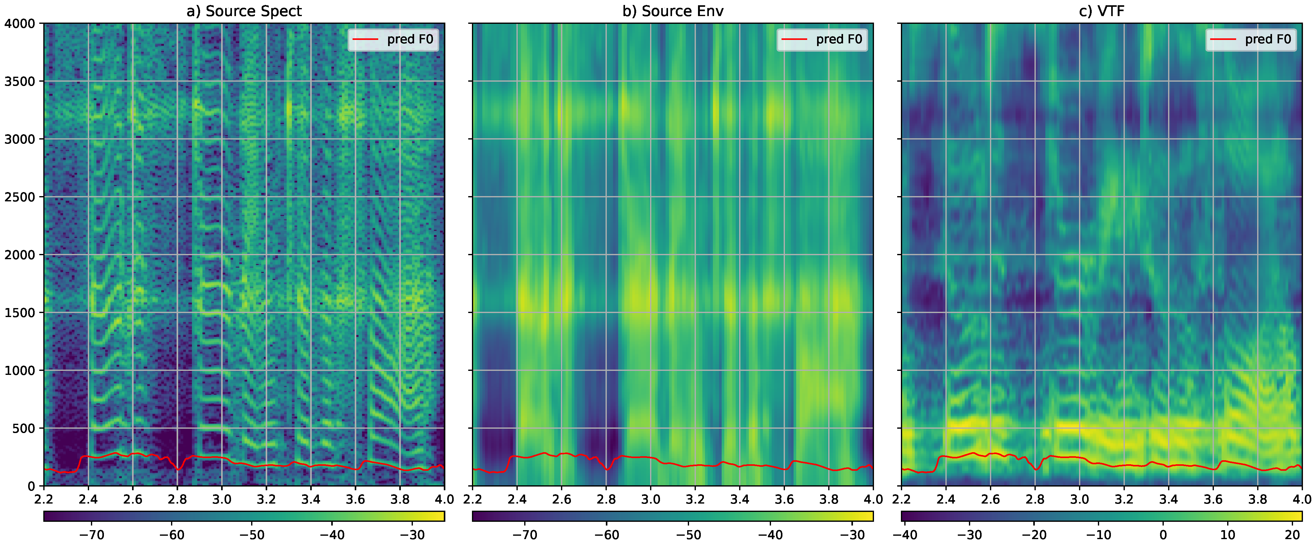
Appendix C. The Effect of the VTF Generator

The ablation study from Section 3.2.3 confirms a positive impact of the VTF Generator of the MBExWN vocoder. Here the question arises how the model separates source and filter components. In the following we will investigate the source-filter decomposition performed by the model using as an example a sub-segment of the phrase LJ007-0048 of the LJSpeech database [54]. The source component generated for this signal segment by means of the Source Generator in Figure 1 is displayed in Figure A1a. The F0 contour predicted by the F0-Net is superimposed on the spectrogram as a red line. The harmonic structure generated according to the predicted F0 is clearly visible. We note that due to the adaptive normalization described in Section 2.3 the energy variation over time is quite weak. The spectral envelope of this signal segment is shown in Figure A1b. This envelope has been estimated using the cepstral domain spectral envelope estimator [46] with frequency resolution set to 200 Hz. The spectral envelope does not show a formant structure but instead shows horizontal stripes at about 1600 Hz and 3200 Hz. Not visible in these band-limited images is the fact that these stripes are part of a periodic structure with a periodicity of approximately 1600 Hz that extends up to Nyquist. This periodic structure is due to the fact that the overall transfer function of the PQMF synthesis filter shown in Figure 2 does contain a periodic 3 dB amplification around the transition bands. In Figure A1c we show the VTF generated by the MBExWN VTF module. Here, we find that the harmonic structure is not fully separated from the VTF. Notably, for segments with F0 above 200 Hz, the harmonic structure is clearly visible. Furthermore, we also find a frequency periodic attenuation that compensates for the frequency periodic amplification in the source signal due to the PQMF synthesis filter. Clearly, the source-filter separation does not establish the separation expected in a classical speech vocoder. A few comments are in order. As mentioned in the introduction the source-filter decomposition is ambiguous. Besides ensuring that the filter preserves energy, Equation (4), nothing prevents the model from moving gain factors for small bands between source and filter. Nevertheless, the Figure A1b shows that besides the effect of the PQMF synthesis filter, the source component remains relatively flat. The MBExWN vocoder does not seem to require using a dedicated source envelope regularization as the one proposed in the Ref. [70]. We explain the fact that the source remains well behaved by the fact that the VTF-Net is much smaller and much simpler to train. Accordingly the model will tend to use the WaveNet only, for those effects that the VTF-Net cannot represent. More problematic is the fact that the harmonic structure appears in the VTF displayed in Figure A1c. This can be explained quite easily as follows. As shown in the Ref. [46] the frequency resolution of a cepstral filter representation can be linked to the number of cepstral coefficients by means of
Δ F = 0.5 F s O T E .
Here Δ F is the frequency resolution, F s is the sampling rate, and O T E is the order of the cepstral model. For our setup the frequency resolution of the VTF filter with 240 coefficients is Δ F = 50 Hz. This frequency resolution is required to represent the speech formants, notably the first one that may have a bandwidth of that order. Accordingly, if we want the VTF module to be able to represent speech formats this implies that it also may represent the harmonic structure. In our initial experiments, we have been able to prevent this situation by means of adding a loss that follows [46] and uses a variant of Equation (A2) to limit the maximum number of cepstral coefficients as a function of the target F0. While the loss succeeds to remove the harmonic structure from the VTF the overall reconstruction error increases slightly, and for some cases, the synthesized signal is perceived as if some vowels are somewhat nasalized. We did interpret this as a result of the model having a problem reproducing the narrow formants. The perceptual evaluation also reveals that the presence of the harmonic structure in the VTF does not produce any perceivable degradation and therefore, in the final MBExWN vocoder, we did not constrain the cepstral order as a function of the F0.
Figure A1. Visualization of the source filter components generated by the MBExWN model. The red line visible in all figures is the F0 predicted by the F0 component. (a) The spectrogram of the source signal generated by the PostNet. (b) The estimate of the spectral envelope of the source signal. (c) The VTF generated in the VTF model of the MBExWN model.
Information 13 00103 g0a1
Another observation that can be made in Figure A1 is the fact that the periodic attenuation/amplification linked to the PWMF filter does not seem to be present at all time positions. The amplification of the source signal seems to be weaker at 3200 Hz and time position 3.8 s and correspondingly the attenuation is weaker in the VTF at the same location. We see this coherent modification of the source signal and the VTF as a positive result that indicates that the coupling of source and filter is working correctly, even if here the model does use it to fix a problem that is produced by the PQMF component. We note that the periodic amplification could be easily prevented by means of a constant filter, but this optimization did not seem justified given the model handles this rather stable effect quite well.

References

  1. Dudley, H. Remaking Speech. J. Acoust. Soc. Am. 1939, 11, 169–177. [Google Scholar] [CrossRef]
  2. Flanagan, J.L.; Golden, R.M. Phase Vocoder. Bell Syst. Tech. J. 1966, 45, 1493–1509. [Google Scholar] [CrossRef]
  3. McAulay, R.J.; Quatieri, T.F. Speech Analysis-Synthesis Based on a Sinusoidal Representation. IEEE Trans. Acoust. Speech Signal Process. 1986, 34, 744–754. [Google Scholar] [CrossRef] [Green Version]
  4. Moulines, E.; Charpentier, F. Pitch-Synchronous Waveform Processing Techniques for Text-to-Speech Synthesis Using Diphones. Speech Commun. 1990, 9, 453–467. [Google Scholar] [CrossRef]
  5. Quatieri, T.F.; McAulay, R.J. Shape Invariant Time-Scale and Pitch Modification of Speech. IEEE Trans. Signal Process. 1992, 40, 497–510. [Google Scholar] [CrossRef]
  6. Kawahara, H.; Masuda-Katsuse, I.; de Cheveigné, A. Restructuring Speech Representations Using a Pitch-Adaptive Time-Frequency Smoothing and an Instantaneous-Frequency-Based F0extraction: Possible Role of a Repetitive Structure in Sounds. Speech Commun. 1999, 27, 187–208. [Google Scholar] [CrossRef]
  7. Kawahara, H.; Morise, M.; Takahashi, T.; Nisimura, R.; Irino, T.; Banno, H. TANDEM-STRAIGHT: A temporally stable power spectral representation for periodic signals and applications to interference-free spectrum, F0, and aperiodicity estimation. In Proceedings of the IEEE International Conference on Acoustics, Speech and Signal Processing (ICASSP 2008), Las Vegas, USA, 30 March–4 April 2008; pp. 3933–3936. [Google Scholar]
  8. Zen, H.; Tokuda, K.; Black, A.W. Statistical Parametric Speech Synthesis. Speech Commun. 2009, 51, 1039–1064. [Google Scholar] [CrossRef]
  9. Röbel, A. Shape-Invariant Speech Transformation with the Phase Vocoder. In Proceedings of the International Conference on Spoken Language Processing (INTERSPEECH 2010), Makuhari, Japan, 26–30 September 2010; pp. 2146–2149. [Google Scholar]
  10. Degottex, G.; Lanchantin, P.; Roebel, A.; Rodet, X. Mixed Source Model and Its Adapted Vocal-Tract Filter Estimate for Voice Transformation and Synthesis. Speech Commun. 2013, 55, 278–294. [Google Scholar] [CrossRef]
  11. Morise, M.; Yokomori, F.; Ozawa, K. WORLD: A Vocoder-Based High-Quality Speech Synthesis System for Real-Time Applications. IEICE Trans Inf. Syst. 2016, 99, 1877–1884. [Google Scholar] [CrossRef] [Green Version]
  12. Markel, J.D.; Gray, A.H. Linear Prediction of Speech; Springer: Berlin/Heidelberg, Germany, 1976. [Google Scholar]
  13. Fant, G. The Source Filter Concept in Voice Production. STL-QPSR Dept Speech Music Hear. KTH 1981, 22, 21–37. [Google Scholar]
  14. Rothenberg, M. Acoustic interaction between the glottal source and the vocal tract. In Vocal Fold Physiology; Stevens, K.N., Hirano, M., Eds.; University of Tokyo Press: Tokyo, Japan, 1981; pp. 305–323. [Google Scholar]
  15. Titze, I.R. Nonlinear Source–Filter Coupling in Phonation: Theory. J. Acoust. Soc. Am. 2008, 123, 1902–1915. [Google Scholar] [CrossRef] [PubMed] [Green Version]
  16. Shen, J.; Pang, R.; Weiss, R.J.; Schuster, M.; Jaitly, N.; Yang, Z.; Chen, Z.; Zhang, Y.; Wang, Y.; Skerrv-Ryan, R.; et al. Natural TTS synthesis by conditioning wavenet on MEL spectrogram predictions. In Proceedings of the 2018 IEEE International Conference on Acoustics, Speech, and Signal Processing (ICASSP 2018), Calgary, AB, Canada, 15–20 April 2018; pp. 4779–4783. [Google Scholar] [CrossRef] [Green Version]
  17. van den Oord, A.; Li, Y.; Babuschkin, I.; Simonyan, K.; Vinyals, O.; Kavukcuoglu, K.; van den Driessche, G.; Lockhart, E.; Cobo, L.C.; Stimberg, F.; et al. Parallel WaveNet: Fast High-Fidelity Speech Synthesis. arXiv 2017, arXiv:1711.10433. [Google Scholar]
  18. Prenger, R.; Valle, R.; Catanzaro, B. Waveglow: A flow-based generative network for speech synthesis. In Proceedings of the International Conference on Acoustics, Speech, and Signal Processing (ICASSP), Brighton, UK, 12–17 May 2019; pp. 3617–3621. [Google Scholar] [CrossRef] [Green Version]
  19. Wang, X.; Takaki, S.; Yamagishi, J. Neural Source-Filter Waveform Models for Statistical Parametric Speech Synthesis. IEEEACM Trans. Audio Speech Lang. Process. 2020, 28, 402–415. [Google Scholar] [CrossRef]
  20. Yamamoto, R.; Song, E.; Kim, J.M. Parallel wavegan: A fast waveform generation model based on generative adversarial networks with multi-resolution spectrogram. In Proceedings of the 2020 IEEE International Conference on Acoustics, Speech, and Signal Processing (ICASSP 2020), Barcelona, Spain, 4–8 May 2020; pp. 6199–6203. [Google Scholar] [CrossRef] [Green Version]
  21. Yang, G.; Yang, S.; Liu, K.; Fang, P.; Chen, W.; Xie, L. Multi-band melgan: Faster waveform generation for high-quality text-to-speech. In Proceedings of the 2021 IEEE Spoken Language Technology Workshop (SLT 2021), Shenzhen, China, 19–22 January 2021; pp. 492–498. [Google Scholar] [CrossRef]
  22. Lorenzo-Trueba, J.; Drugman, T.; Latorre, J.; Merritt, T.; Putrycz, B.; Barra-Chicote, R.; Moinet, A.; Aggarwal, V. Towards Achieving Robust Universal Neural Vocoding. In Proceedings of the 20th Annual Conference of the International Speech Communication Association (INTERSPEECH 2019), Graz, Austria, 15–19 September 2019; pp. 181–185. [Google Scholar] [CrossRef] [Green Version]
  23. Jang, W.; Lim, D.; Yoon, J. Universal MelGAN: A Robust Neural Vocoder for High-Fidelity Waveform Generation in Multiple Domains. arXiv 2021, arXiv:2011.09631. [Google Scholar]
  24. Jiao, Y.; Gabryś, A.; Tinchev, G.; Putrycz, B.; Korzekwa, D.; Klimkov, V. Universal neural vocoding with parallel wavenet. In Proceedings of the 2021 IEEE International Conference on Acoustics, Speech, and Signal Processing (ICASSP 2021), Toronto, ON, Canada, 6–11 June 2021; pp. 6044–6048. [Google Scholar] [CrossRef]
  25. Ping, W.; Peng, K.; Gibiansky, A.; Arik, S.O.; Kannan, A.; Narang, S.; Raiman, J.; Miller, J. Deep Voice 3: Scaling Text-to-Speech with Convolutional Sequence Learning. arXiv 2018, arXiv:1710.07654. [Google Scholar]
  26. Zhang, J.X.; Ling, Z.H.; Dai, L.R. Non-Parallel Sequence-to-Sequence Voice Conversion with Disentangled Linguistic and Speaker Representations. IEEEACM Trans. Audio Speech Lang. Process. 2020, 28, 540–552. [Google Scholar] [CrossRef]
  27. Qian, K.; Zhang, Y.; Chang, S.; Yang, X.; Hasegawa-Johnson, M. AutoVC: Zero-shot voice style transfer with only autoencoder loss. In Proceedings of the International Conference on Machine Learning, Long Beach, CA, USA, 9–15 June 2019; pp. 5210–5219. [Google Scholar]
  28. Qian, K.; Zhang, Y.; Chang, S.; Hasegawa-Johnson, M.; Cox, D. Unsupervised speech decomposition via triple Information Bottleneck. In Proceedings of the 37th International Conference on Machine Learning, Virtual, 13–18 July 2020; pp. 7836–7846. [Google Scholar]
  29. Benaroya, L.; Obin, N.; Roebel, A. Beyond Voice Identity Conversion: Manipulating Voice Attributes by Adversarial Learning of Structured Disentangled Representations. arXiv 2021, arXiv:2107.12346. [Google Scholar]
  30. Desler, A. ‘Il Novello Orfeo’ Farinelli: Vocal Profile, Aesthetics, Rhetoric. Ph.D. Thesis, University of Glasgow, Glasgow, UK, 2014. [Google Scholar]
  31. Lample, G.; Zeghidour, N.; Usunier, N.; Bordes, A.; Denoyer, L.; Ranzato, M. Fader Networks:Manipulating Images by Sliding Attributes. In Proceedings of the 31st Conference on Neural Information Processing Systems (NIPS 2017), Long Beach, CA, USA, 4–9 December 2017; pp. 5967–5976. [Google Scholar]
  32. He, Z.; Zuo, W.; Kan, M.; Shan, S.; Chen, X. AttGAN: Facial Attribute Editing by Only Changing What You Want. IEEE Trans. Image Process. 2019, 28, 5464–5478. [Google Scholar] [CrossRef] [Green Version]
  33. Collins, E.; Bala, R.; Price, B.; Susstrunk, S. Editing in style: Uncovering the local semantics of GANs. In Proceedings of the 2020 IEEE/CVF Conference on Computer Vision and Pattern Recognition (CVPR), Seattle, WA, USA, 13–19 June 2020; pp. 5770–5779. [Google Scholar] [CrossRef]
  34. Engel, J.; Hantrakul, L.; Gu, C.; Roberts, A. DDSP: Differentiable Digital Signal Processing. arXiv 2020, arXiv:2001.04643. [Google Scholar]
  35. Engel, J.; Hantrakul, L.; Gu, C.; Roberts, A. DDSP Software. Available online: https://github.com/magenta/ddsp (accessed on 22 December 2021).
  36. Serra, X.J.; Smith, J.O. Spectral Modeling Synthesis: A Sound Analysis/Synthesis System Based on a Deterministic plus Stochastic Decomposition. Comput. Music J. 1990, 14, 12–24. [Google Scholar] [CrossRef]
  37. Song, E.; Byun, K.; Kang, H.G. ExcitNet vocoder: A neural excitation model for parametric speech synthesis systems. In Proceedings of the 2019 IEEE 27th European Signal Processing Conference (EUSIPCO), Coruna, Spain, 2–6 September 2019; pp. 1–5. [Google Scholar]
  38. Juvela, L.; Bollepalli, B.; Tsiaras, V.; Alku, P. GlotNet—A Raw Waveform Model for the Glottal Excitation in Statistical Parametric Speech Synthesis. IEEEACM Trans. Audio Speech Lang. Process. 2019, 27, 1019–1030. [Google Scholar] [CrossRef]
  39. Juvela, L.; Bollepalli, B.; Yamagishi, J.; Alku, P. GELP: GAN-excited liner prediction for speech synthesis from mel-spectrogram. In Proceedings of the International Speech Communication Association (Interspeech 2019), Graz, Austria, 15–19 September 2019; pp. 694–698. [Google Scholar]
  40. Oh, S.; Lim, H.; Byun, K.; Hwang, M.J.; Song, E.; Kang, H.G. ExcitGlow: Improving a WaveGlow-based Neural Vocoder with Linear Prediction Analysis. In Proceedings of the IEEE 2020 Asia-Pacific Signal and Information Processing Association Annual Summit and Conference (APSIPA ASC), Auckland, New Zealand, 7–10 December 2020; pp. 831–836. [Google Scholar]
  41. Roebel, A.; Bous, F. Towards Universal Neural Vocoding with a Multi-band Excited WaveNet. arXiv 2021, arXiv:2110.03329. [Google Scholar]
  42. Aitken, A.; Ledig, C.; Theis, L.; Caballero, J.; Wang, Z.; Shi, W. Checkerboard Artifact Free Sub-Pixel Convolution: A Note on Sub-Pixel Convolution, Resize Convolution and Convolution Resize. arXiv 2017, arXiv:1707.02937. [Google Scholar]
  43. Salimans, T.; Goodfellow, I.; Zaremba, W.; Cheung, V.; Radford, A.; Chen, X. Improved techniques for training gans. In Proceedings of the Advances in Neural Information Processing Systems, Barcelona, Spain, 5–10 December 2016; pp. 2234–2242. [Google Scholar]
  44. Van den Oord, A.; Dieleman, S.; Zen, H.; Simonyan, K.; Vinyals, O.; Graves, A.; Kalchbrenner, N.; Senior, A.; Kavukcuoglu, K. WaveNet: A generative model for raw audio. In Proceedings of the 9th ISCA Speech Synthesis Workshop, Sunnyvale, CA, USA, 13–15 September 2016; p. 125. [Google Scholar]
  45. Smith, J.O. Spectral Audio Signal Processing. 2011. Available online: https://ccrma.stanford.edu/~jos/sasp (accessed on 10 May 2021).
  46. Röbel, A.; Villavicencio, F.; Rodet, X. On Cepstral and All-Pole Based Spectral Envelope Modeling with Unknown Model Order. Pattern Recognit. Lett. Spec. Issue Adv. Pattern Recognit. Speech Audio Process. 2007, 28, 1343–1350. [Google Scholar] [CrossRef]
  47. Smith, J.O. Introduction to Digital Filters with Audio Applications. 2007. Available online: https://ccrma.stanford.edu/~jos/filters/filters.html (accessed on 10 May 2021).
  48. Yu, C.; Lu, H.; Hu, N.; Yu, M.; Weng, C.; Xu, K.; Liu, P.; Tuo, D.; Kang, S.; Lei, G. DurIAN: Duration Informed Attention Network for Speech Synthesis. In Proceedings of the 21st Annual Conference of the International Speech Communication Association (INTERSPEECH 2020), Shanghai, China, 25–29 October 2020; pp. 2027–2031. [Google Scholar]
  49. Lin, Y.P.; Vaidyanathan, P. A Kaiser Window Approach for the Design of Prototype Filters of Cosine Modulated Filterbanks. IEEE Signal Process. Lett. 1998, 5, 132–134. [Google Scholar] [CrossRef] [Green Version]
  50. Shanker, M.; Hu, M.Y.; Hung, M.S. Effect of Data Standardization on Neural Network Training. Omega 1996, 24, 385–397. [Google Scholar] [CrossRef]
  51. McFee, B. Librosa—Librosa 0.8.1 Documentation. 2021. Available online: https://librosa.org/doc/latest/index.html#id1 (accessed on 5 October 2021).
  52. Griffin, D.; Lim, J. Signal Estimation from Modified Short-Time Fourier Transform. IEEE Trans. Acoust. Speech Signal Process. 1984, 32, 236–243. [Google Scholar] [CrossRef]
  53. Kingma, D.P.; Ba, J.L. Adam: A Method for Stochastic Optimization. In Proceedings of the International Conference on Learning Representations, San Diego, CA, USA, 7–9 May 2015. [Google Scholar]
  54. Ito, K.; Johnson, L. The LJ Speech Dataset. 2017. Available online: https://keithito.com/LJ-Speech-Dataset (accessed on 10 May 2021).
  55. Yamagishi, J.; Veaux, C.; MacDonald, K. CSTR VCTK Corpus: English Multi-Speaker Corpus for CSTR Voice Cloning Toolkit (Version 0.92). 2019. Available online: https://datashare.ed.ac.uk/handle/10283/3443 (accessed on 5 October 2021). [CrossRef]
  56. Pirker, G.; Wohlmayr, M.; Petrik, S.; Pernkopf, F. A Pitch Tracking Corpus with Evaluation on Multipitch Tracking Scenario. In Proceedings of the 12th Annual Conference of the International Speech Communication Association (INTERSPEECH 2011), Florence, Italy, 27–31 August 2011; pp. 1509–1512. [Google Scholar]
  57. Le Moine, C.; Obin, N. Att-HACK: An Expressive Speech Database with Social Attitudes. In Proceedings of the 10th International Conference on Speech Prosody, Tokyo, Japan, 25–28 May 2020. [Google Scholar]
  58. Grammalidis, N.; Dimitropoulos, K.; Tsalakanidou, F.; Kitsikidis, A.; Roussel, P.; Denby, B.; Chawah, P.; Buchman, L.; Dupont, S.; Laraba, S.; et al. The I-treasures intangible cultural heritage dDataset. In Proceedings of the 3rd International Symposium on Movement and Computing, Thessaloniki, Greece, 5–6 July 2016; Association for Computing Machinery: New York, NY, USA, 2016; pp. 1–8. [Google Scholar] [CrossRef]
  59. Duan, Z.; Fang, H.; Li, B.; Sim, K.C.; Wang, Y. The NUS sung and spoken lyrics corpus: A quantitative comparison of singing and speech. In Proceedings of the 2013 Asia-Pacific Signal and Information Processing Association Annual Summit and Conference, Kaohsiung, Taiwan, 29 October–1 November 2013; pp. 1–9. [Google Scholar]
  60. Tsirulnik, L.; Dubnov, S. Singing voice database. In Proceedings of the International Conference on Speech and Computer, Istanbul, Turkey, 20–25 August 2019; pp. 501–509. [Google Scholar]
  61. Koguchi, J.; Takamichi, S.; Morise, M. PJS: Phoneme-balanced Japanese singing-voice corpus. In Proceedings of the 2020 Asia-Pacific Signal and Information Processing Association Annual Summit and Conference (APSIPA ASC), Auckland, New Zealand, 7–10 December 2020; pp. 487–491. [Google Scholar]
  62. Tamaru, H.; Takamichi, S.; Tanji, N.; Saruwatari, H. JVS-MuSiC: Japanese Multispeaker Singing-Voice Corpus. arXiv 2020, arXiv:2001.07044. [Google Scholar]
  63. Ogawa, I.; Morise, M. Tohoku Kiritan Singing Database: A Singing Database for Statistical Parametric Singing Synthesis Using Japanese Pop Songs. Acoust. Sci. Technol. 2021, 42, 140–145. [Google Scholar] [CrossRef]
  64. Zen, H.; Dang, V.; Clark, R.; Zhang, Y.; Weiss, R.J.; Jia, Y.; Chen, Z.; Wu, Y. LibriTTS: A Corpus Derived from LibriSpeech for Text-to-Speech. arXiv 2019, arXiv:1904.02882. [Google Scholar]
  65. Ardaillon, L.; Roebel, A. Fully-Convolutional Network for Pitch Estimation of Speech Signals. In Proceedings of the 20th Annual Conference of the International Speech Communication Association (INTERSPEECH 2019), Graz, Austria, 15–19 September 2019; pp. 2005–2009. [Google Scholar] [CrossRef] [Green Version]
  66. Roebel, A. SuperVP Software. 2015. Available online: http://anasynth.ircam.fr/home/english/software/supervp (accessed on 31 January 2021).
  67. Huber, S.; Roebel, A. On glottal source shape parameter transformation using a novel deterministic and stochastic speech analysis and synthesis system. In Proceedings of the 16th Annual Conference of the International Speech Communication Association (Interspeech 2015), Dresden, Germany, 6–10 September 2015. [Google Scholar] [CrossRef]
  68. Rafii, Z.; Liutkus, A.; Stöter, F.R.; Mimilakis, S.; Bittner, R. The MUSDB18 Corpus for Music Separation. 2017. Available online: https://sigsep.github.io/datasets/musdb.html (accessed on 31 January 2021).
  69. Roebel, A.; Bous, F. MBExWN_Vocoder. 2022. Available online: https://github.com/roebel/MBExWN_Vocoder (accessed on 8 February 2022).
  70. Yoneyama, R.; Wu, Y.C.; Toda, T. Unified Source-Filter GAN: Unified Source-filter Network Based On Factorization of Quasi-Periodic Parallel WaveGAN. arXiv 2021, arXiv:2104.04668. [Google Scholar]
Figure 1. MBExWN schematic generator: Green boxes are DNN models, yellow boxes are differentiable DSP operators, red ovals are losses. The numbers below the boxes designate the output dimension of the respective box in the format time × channels (batch dimension not shown) for a single mel frame as input (dimensions 1 × 80 ). In the present study, the mel frame hop size is 300 samples @ 24 kHz and therefore the model needs to achieve an overall upsampling factor of 300.
Information 13 00103 g001
Figure 2. The 15-band PQMF filter transfer function used in the study. The figure shows the individual filter transfer functions and the sum of all individual transfer functions (the sum is in brown).
Information 13 00103 g002
Figure 3. Adaptive normalization applied to a short segment of a speech signal. (a) Short segment of original speech signal. (b) Signal after normalization using g n ( 2 ) with E ^ M obtained from Equation (17) (note the change in vertical axis limits). (c) The same as in (b) but using energy estimation from Equation (16). (d) Mel spectrogram of original sound for the segment displayed in (a). (e) Mel spectrogram M ( 2 ) of sound segment in (b). (f) Visualization of the incoherence as the difference between the mel spectrogram from (e) and the mel spectrogram M + ( 2 ) obtained by means of shifting mel frames in (d).
Information 13 00103 g003
Figure 4. Comparison of mel spectrogram reconstruction errors for models trained with adaptive mel normalization and random gain augmentation on a short segment of a speech signal. (a) Mel spectrogram of original speech signal in dB. (b) Mel spectrogram after reconstruction with MBExWn model trained with adaptive normalization with smoothing window size α = 2 and one smoothing iteration. (c) Difference between (a,b). (d) Mel spectrogram after reconstruction with MBExWN model trained with random gain attenuation under gain augmentation with γ = 0.1 . (e) Difference between (a,d).
Information 13 00103 g004
Table 1. Inconsistency measures δ ( i ) and Δ ( i ) between the normalized mel spectrogram and mel spectrogram calculated from the audio signal normalized time.
Diff Measure/Iteration i = 0 i = 1 i = 2 i = 3 i = 4 i = 5
Normalization using Equation (17)
δ ( i ) [dB]1.140.590.430.360.310.28
Δ ( i ) [dB]21.7011.157.236.035.564.91
Normalization using Equation (16)
δ ( i ) [dB]1.180.630.470.390.340.30
Δ ( i ) [dB]20.868.986.495.554.884.50
Table 2. Results of the ablation study. The mel reconstruction error is shown together with the 95% confidence intervals.
MBExWN ConfigurationMel Error [dB]
Default 1.392 ± 0.015
WT+PQMF 1.419 ± 0.014
Default-2S 1.434 ± 0.011
No PQMF 1.481 ± 0.017
No VTF 1.731 ± 0.021
Table 3. Average rating and standard deviation for the perceptual evaluation of the perceived difference between original and resynthesis using different variants of the MBExWN model. The test data contains unseen phrases from voice identities (speakers/singers) that were used during training.
Data\ModelHREFMW-SP-FDMW-SI-FDMW-VO-FDMW-VO-FR
SP96 (1.7)86 (5.0)-82 (5.9)62 (7.4)
SI95 (1.8)-82 (6.1)91 (3.3)80 (6.0)
Table 4. Average rating and standard deviation for the perceptual evaluation of the perceived difference between original and resynthesis for the speech and all-purpose variants of the MBExWN model. The test data is taken from data sets containing voice identities that where never seen by the MBExWN models. For the base line models UMG-LJ+LT-FD and MMG-LJ-FD the voice identity LJ was part of the training data set.
Data\ModelHREFMW-SP-FDMW-VO-FDUMG-LJ+LT-FDMMG-LJ-FD
LJ94 (1.9)85 (4.3)82 (5.2)-86 (4.1)
UMG(LJ)93 (3.7)86 (6.8)77 (11.4)80 (10.6)-
UMG(others)94 (2.2)78 (6.4)74 (7.5)81 (6.3)-
Table 5. Average rating and standard deviation for the perceptual evaluation of the perceived difference between original and resynthesis for different variants of the MBExWN model and a multi-band MelGAN baseline.
Data\ModelHREFMW-SI-FDMW-VO-FDMMG-DI-FD
DI94 (2.7)83 (8.4)86 (6.2)85 (5.5)
Pop(MusDB)93 (2.7)73 (8.3)79 (8.1)-
Rough96 (2.7)60 (12.7)68 (11.3)-
Publisher’s Note: MDPI stays neutral with regard to jurisdictional claims in published maps and institutional affiliations.

