Robust Segmentation Based on Salient Region Detection Coupled Gaussian Mixture Model

Abstract

The impressive progress on image segmentation has been witnessed recently. In this paper, an improved model introducing frequency-tuned salient region detection into Gaussian mixture model (GMM) is proposed, which is named FTGMM. Frequency-tuned salient region detection is added to achieve the saliency map of the original image, which is combined with the original image, and the value of the saliency map is added into the Gaussian mixture model in the form of spatial information weight. The proposed method (FTGMM) calculates the model parameters by the expectation maximization (EM) algorithm with low computational complexity. In the qualitative and quantitative analysis of the experiment, the subjective visual effect and the value of the evaluation index are found to be better than other methods. Therefore, the proposed method (FTGMM) is proven to have high precision and better robustness.

1. Introduction

In the field of computer vision, image segmentation is a basic and inevitable technology to analyze the scene [1]. The definition of image segmentation is to divide the image into regions with consistent attributes and different statistical characteristics [2,3,4]. Accurate segmentation results are conducive to feature extraction and recognition classification of the target in the later stage. People regard image segmentation as the most important low-level work in the field of computer vision, which is a steppingstone to better complete the research work in the image. The reason why image segmentation is valued by people is that it can’t be underestimated in the actual scene application value. For example, in the road scenario study [5], the road scenes are split into some parts, so as to predict the obstacles and pedestrians in front of the road, thus realizing to avoid accidental injury. In the supermarket environment, the reliable segmentation on fruit and vegetables [6] at a supermarket is needed, which can help supermarket workers sort fruits and vegetables quickly. In the medical field, patients are involved in the segmentation of tumors and other lesions by carrying out B-ultrasound, computer tomography (CT) and other examinations. Medical imaging plays an important role in doctors’ understanding of the lesions, which is related to life. Therefore, how to achieve accurate segmentation of tumors [5,6] and other lesions in the medical images requires the intervention of image segmentation technology. In addition, face recognition [7] of facial features is used for real-time face acquisition in the security system [8], in order to find out the people and things needed for the related work in the future. As mentioned above, image segmentation technology has been closely related to people’s daily life. Therefore, it is very important to improve the image segmentation technology and improve the segmentation performance of the method.

According to the development of image segmentation, it is divided into non-deep learning and deep learning. Traditional segmentation methods are regarded as non-deep learning. They are divided into three categories: threshold method [9], edge segmentation [10] and region segmentation [11]. The threshold method is divided into single threshold segmentation and multi-value segmentation. The methods of edge segmentation include the edge detection method and boundary growing way. The methods based on region segmentation are divided into the region growing method and the region splitting merging method. The second kind of non-deep learning method is the segmentation method based on specific theory [12,13,14,15,16], which is divided into several categories: clustering segmentation, based on mathematical morphology, fuzzy sets theory, wavelet transform, energy function and statistics. Common clustering segmentation includes K-means segmentation and fuzzy set c-means segmentation. Statistical methods include the finite mixture model and Markov model [17,18,19,20,21,22,23]. There are three kinds of segmentation methods based on deep learning: semantic segmentation [24], instance segmentation [25] and panoramic segmentation [26].

The method in this paper is based on the research branch of finite mixture model, which belongs to the category of traditional image segmentation. Through the analysis of related work, the main problems existing in this type of method are as follows: most of the existing segmentation algorithms fail to take the context information of image pixels into consideration, which leads to imprecisely deciding the spatial neighborhood information of the pixels. In addition, the continuity of the image pixels is also affected.

In order to solve those problems, an improved model combining frequency-tuned salient region detection to Gaussian mixture model (GMM) is proposed in this paper. The spatial information of pixels is considered in combination with saliency, which is introduced into the target model in the form of weight. Therefore, the deficiency that most methods fail to consider the context information of pixels is solved. In addition, we use the expectation maximization algorithm combined with the logarithmic likelihood function to solve the parameters, in order to find the optimal solution of the model, to achieve high precision and good robustness of image segmentation. In our experiment, we conducted experimental analysis on data in a variety of scenarios and achieved good results in quantitative and qualitative analysis.

The main contributions in this paper are as follows: (1) an efficient method combining frequency-tuned salient region detection to Gaussian mixture model is proposed in this paper, this saliency reflects the context information of the image pixels, edge information and indistinguishable pixels are protected so that they can be classified and judged by the influence of adjacent pixels; (2) frequency-tuned salient region detection is introduced to obtain the saliency map of the original image, and the saliency map value is added into the Gaussian mixture model in the form of spatial information weight. The mapping value of the significance part can be solved independently, which reduces the computational complexity; and (3) the proposed method FTGMM not only solves the model parameters based on the EM algorithm with low computational complexity, but also outperforms the latest experimental results on Berkeley natural datasets and medical images. The segmentation performance in different scenarios can be compared to show its optimal.

This paper contains the following parts: Section 2 describes the related work. Section 3 presents the proposed algorithm in detail. In Section 4, the experimental results are shown. Section 5 summarizes this paper, and then finally there are the references.

2. Related Work

The finite mixture model (FMM) is a modeling tool for the statistical modelling of data. It advocates an effective mathematical method of simulating complex density with simple density function, which is due to its flexibility. In 1894, Karl [12] assigned different weights to two univariate Gaussian distribution models, fitted a group of observation data, and estimated the parameter set of the mixture model by the distance estimation method. In 1996, T. K. moon [10] proposed the expectation maximization (EM) algorithm for solving parameters, and EM [14,15,16] is often used to solve the estimation of the mixture model. GMM is more used in image segmentation [17]. The pixels with similar gray values are divided into the same class, so the pixel classification is realized by numerical clustering. However, the traditional GMM ignores the spatial relationship between pixels.

In 2007, A. Diplaros [18] proposed a new spatial constraint, which assumed that the unobserved category labels of adjacent pixels in the image are generated by prior distribution with similar parameters. The hidden Markov model is used to construct the prior spatial prior relationship between pixels. Although Markov random field provides a simple and effective way for image spatial modeling, it has difficult parameter estimation, which is a problem. In 2013, Zhang and Nguyen. T. M. Nguyen [19] applied the Markov random field model as a prior model of parameters and carried out a series of secondary optimization through the constructor. In 2016, Liqiu Chen [20] published a paper proposing a method for dynamic texture segmentation of inter-scale background based on Markov random fields. In 2021, hidden Markov random fields [21] have been proposed. The spatial information relation of pixels is constructed by it, and a new context constraint is formed to carry out image segmentation. This model is also used in brain image segmentation [22,23,24]. When using Markov random fields [23] to process spatial relations, although it shows excellent results, it is often unable to directly use M-step of EM to calculate parameters, and there are too many generated parameters, complex calculations and high calculation costs.

Another way to deal with the spatial relationship of pixels is to use the mean template. In 2009, Tang [24] proposed the neighborhood weighted method, namely GMM-MT, which has a good effect in the results. In 2016, Zhang [25] proposed ACAP. In 2018, a liver segmentation model [26] is proposed using a sequence of modules based on personalized model knowledge of liver appearance and shape. In 2021, a new EM algorithm [27] for GMMs has been proposed. It further optimizes the solution process of the Gaussian mixture model and improves the method. In these methods, the probability weighting of the mean template is calculated by the geometric mean weighted template and arithmetic mean template. This method has a good effect on noise robustness and is faster. However, the key problem is that the context information of independent pixels is not considered.

Recently, the saliency map is concerned. In 2018, Bi [28] proposed the GMM-SMSI method. This method introduced the saliency map as a weight into the GMM through the saliency detection method spectral residual method proposed by Hou [29] so that the prior probability of the current pixel can be estimated by the saliency weight of the neighboring pixels, and fully reflects the context of the image information. Compared with the method of constructing Gaussian pyramid to obtain saliency map proposed by Itti [30,31,32], the above method is simpler in terms of computational complexity. Frequency-tuned saliency extraction [33] is simpler and only needs Gaussian smoothing and mean calculation, which outputs full resolution saliency map with a clear boundary. This method makes use of the characteristics of color and brightness, so it is easy to implement and has high computational efficiency. Based on this consideration, this paper proposes the use of the FT saliency extraction method to extract saliency. Figure 1 shows the difference between the traditional Gaussian mixture model segmentation and the process described in this paper.

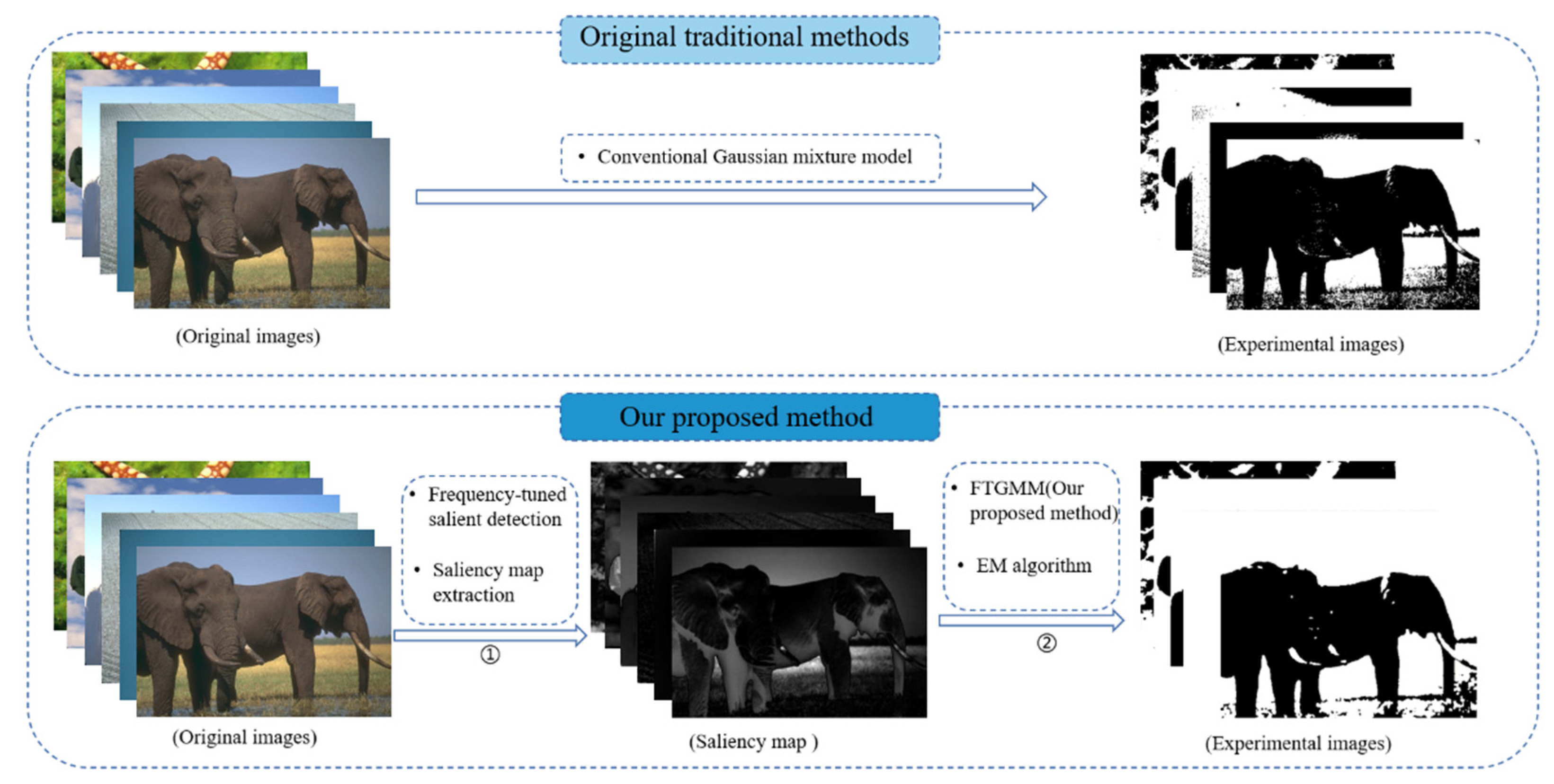
3. Proposed Algorithm

3.1. Gaussian Mixture Model

In the method of image segmentation based on specific theory, the method of segmentation based on statistics is often referred to as the finite mixture model (FMM). The finite mixture model (FMM) is widely used in image segmentation. It has been formally proposed since FMM in 2000. The commonly used mathematical model is shown in Equation (1):

$$p\left(x_i|\theta \right)={\displaystyle \sum }_{k=1}^K {\pi }_k p\left(x_i|{\theta }_k\right)$$

(1)

where $p\left(x_i|\theta \right)$ is a function which is used to fit image histogram, K is the total number of tags of different categories. ${\pi }_k$ is the weight of each distribution density function in the overall model, $p\left(x_i|{\theta }_k\right)$ is the expression of the $i$-th distribution function. The distribution of pixels can be outlined by Gaussian distribution, which is regarded as the distribution density function in the finite mixture model (FMM). The expression of Gaussian distribution is:

$$\Phi \left(x|\mu , \Sigma \right)=\frac{1}{{\left(2\pi \right)}^{D/2}{\left|\Sigma \right|}^{1/2}}exp\left\{-\frac{1}{2}{\left(x-\mu \right)}^T{\Sigma }^{-1}\left(x-\mu \right)\right\}$$

(2)

where $x$ shows the value of the sample, namely, the gray value of the pixels, $\mu$ is the mean value of the sample, $\Sigma$ represents the covariance in the Gaussian distribution model, $\exp \{.\}$ is the exponential function based on the natural number e, $T$ is the transposition of vector, $D$ is the dimension. Generally, gray image is two-dimensional image, so D is set as 2. When the input image is an RGB image, which is a three-dimensional image, in order to facilitate the unified processing of the model, when the input image is the RGB image, it needs to perform grayscale conversion to transform it into two-dimensional image. Therefore, the parameter D in our model proposed in this paper is 2 by default. Obeying such a distribution function means obeying Gaussian distribution. Equation (3) represents Gaussian mixture model:

$$f\left(x_i|\Pi ,\Theta \right)={\displaystyle \sum }_{j=1}^L{\pi }_j\Phi \left(x_i|{\theta }_j\right)$$

(3)

where $\Pi =\left\{{\pi }_1,{\pi }_2\dots ,{\pi }_L\right\},\sum _{j=1}^L{\pi }_j=1,\Theta =\left\{{\theta }_1,{\theta }_2,\dots ,{\theta }_L\right\},{\theta }_j=\left\{{\mu }_j,{\Sigma }_j\right\}$, $\Theta$ represents a set of parameters in a Gaussian distribution. L is the total number of tags of different categories.

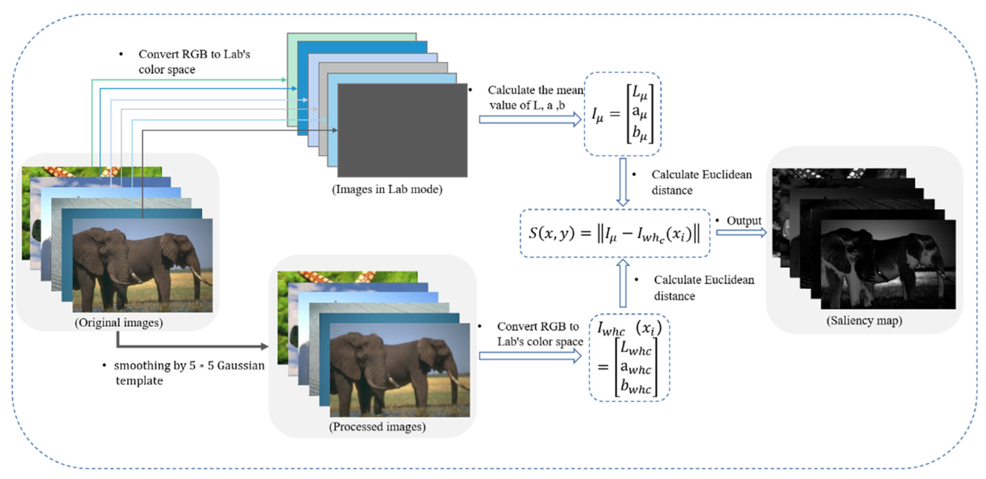
3.2. Extraction of Saliency Map

Saliency map has been widely used in detection. It reflects the regions of interest in the image and contains potential feature information. Image is usually divided into low frequency part and the high frequency part. The low frequency part reflects the overall information of the image, while high frequency reflects the details of the image. R. Achanta [33] proposed a new saliency extraction, namely frequency-tuned (FT) algorithm, which is calculated by the Equation (4):

$$S\left(x_i\right)=||I_{\mu }-I_{w{h}_c}\left(x_i\right)||$$

(4)

In Equation (4), $x_i$ is the $i$-th pixel of the image, $I_{\mu }$ is the average feature vector of the image, using Lab color features, $I_{w{h}_c}\left(x_i\right)$ is the corresponding image pixel feature after 5 × 5 Gaussian blurred version on pixel $x_i$ to round off the highest frequency, ||·|| is $L_2$ normal form. Using the Lab color space, each pixel location is a vector, and the $L_2$ normal is the Euclidean distance. The calculation process is shown in Figure 2.

3.3. Gaussian Mixture Model with Saliency Weight

Gaussian distribution is a probability model, it represents a simple linear combination of Gaussian density, GMM can divide $N$ pixels into $K$ class labels, $i$ represents the index of pixels, $i=\left\{1,2,\dots \dots ,N\right\}$, $j$ is the index of the class label, $j=\left\{1,2,\dots ,L\right\}$. The traditional Gaussian mixture model is shown in Equation (2). The probability of $i$-th pixel belonging to the $j$-th class is given by Equation (2), where ${\theta }_j=\left\{{\mu }_j,{\Sigma }_j\right\}$ represents the mean and covariance of the $j$-th Gaussian distribution. The conventional GMM is shown in Equation (3), where $\Pi$ is the prior probability of pixel distribution, which can also be called mixed component weight. Specifically review Equations (2) and (3). Detailed elaboration of the model in this paper will be expanded in the following paragraphs.

The spatial information reflected by the saliency of the pixel is introduced into GMM in a way of weight. In this paper, the saliency map is used to assign proper weights to the pixels in the original image. The mathematical model is shown in the following Equation (5):

$$f\left(x_i|\Psi \right)={\displaystyle \sum }_{j=1}^L{\pi }_{ij}\left[{\displaystyle \sum }_{m\in N_i}\frac{S\left(x_m\right)}{R_i}p(x_m|{\Theta }_j)\right]$$

(5)

where ${\pi }_{ij}$ represents the prior probability which the pixel $x_i$ is classified as the $j$-th class, $p(x_m|{\Theta }_j)$ represents the $j$-th Gaussian distribution. $N_i$ stands for the neighborhood of $x_i$, $m$ is the pixel index in the $N_i$. $R_i$ is the sum of saliency mapping values of all pixels in the neighborhood. $S\left(x_m\right)$ represents the saliency mapping value of the pixel $x_m$. $\Psi$ represents all the parameters involved in the model. $\Psi =${${\pi }_{11}$, ${\pi }_{12}$,…, ${\pi }_{1L}$, ${\pi }_{21}$, ${\pi }_{22},$ ${\pi }_{2L}$,…$,{\pi }_{N1},{\pi }_{N2}$, …, ${\pi }_{NL}$, ${\Theta }_1,{\Theta }_2,\dots ,{\Theta }_L$}.

In the part of parameter solving, EM algorithm is used to solve and optimize the parameters. According to reference [22], the complete data log likelihood function of the objective function is as follows:

$$Q={\displaystyle \sum }_{i=1}^N{\displaystyle \sum }_{j=1}^L{\gamma }_{ij}\left[{\displaystyle \sum }_{m\in N_i}\frac{S\left(x_m\right)}{R_i}logp\left(x_m|{\tau }_j\right)+log{\pi }_{ij}\right]$$

(6)

In the Equation (6), $Q$ represents the log likelihood function of the objective function. $i=\left\{1,2,\dots \dots ,N\right\}$, which is the index of pixels. $j$ is the index of the class label, $j=\left\{1,2,\dots ,L\right\}$. ${\gamma }_{ij}$ is the posterior probability, which measures the likelihood that an event will happen given that a related event has already occurred.

In the step of seeking expectation, the posterior probability ${\gamma }_{ij}$ is calculated as follows:

$${\gamma }_{ij}^{\left(t\right)}=\frac{{\pi }_{ij}^{\left(t\right)}{\sum }_{m\in N_i}\frac{S\left(x_m\right)}{R_i}p\left(x_m|{\theta }_j^{\left(t\right)}\right)}{{\sum }_{j=1}^L{\pi }_{ij}^{\left(t\right)}{\sum }_{m\in N_i}\frac{S\left(x_m\right)}{R_i}p\left(x_m|{\theta }_j^{\left(t\right)}\right)}$$

(7)

where $t$ is the $t$-th of iterations. ${\gamma }_{ij}^{\left(t\right)}$ represents the posterior probability when the number of iterations is $t$. ${\pi }_{ij}^{\left(t\right)}$ means the prior probability of the $t$-th. $p\left(x_m|{\theta }_j^{\left(t\right)}\right)$ is the expression of the $j$-th distribution function when iteration number is $t$.

In the process of maximizing, the mean and covariance are calculated as follows:

$${\mu }_j^{\left(t+1\right)}=\frac{{\sum }_{i=1}^N{\sum }_{m\in N_i}{\gamma }_{ij}^{\left(t\right)}\frac{S\left(x_m\right)}{R_i}{x}_m}{{\sum }_{i=1}^N{\gamma }_{ij}^{\left(t\right)}}$$

(8)

$${\mathsf{\Sigma }}_j^{\left(t+1\right)}=\frac{{\sum }_{i=1}^N{\sum }_{m\in N_i}{\gamma }_{ij}^{\left(t\right)}\frac{S\left(x_m\right)}{R_i}(x_m-{\mu }_j^{\left(t\right)}){\left(x_m-{\mu }_j^{\left(t\right)}\right)}^{\mathsf{{\rm T}}}}{{\sum }_{i=1}^N{\gamma }_{ij}^{\left(t\right)}}$$

(9)

In the Equations (8) and (9), ${\mu }_j^{\left(t+1\right)}$ and ${\sum }_j^{\left(t+1\right)}$ are on behalf of the mean and covariance in the next iteration. They do calculations and numerical updates based on the results of the previous iteration.

Prior probability ${\pi }_{ij}$ is calculated as follows:

$${\pi }_{ij}^{\left(t+1\right)}=\frac{{\sum }_{m\in N_i}S\left(x_m\right){\gamma }_{mj}^{\left(t\right)}}{{\sum }_{j=1}^L{\sum }_{m\in N_i}S\left(x_m\right){\gamma }_{mj}^{\left(t\right)}}$$

(10)

In the Equation (10), through the combination of the $i$-th pixel and its neighborhood pixel processing, calculate the prior probability of the next time, namely, ${\pi }_{ij}^{\left(t+1\right)}.$

4. Experiments

This section mainly shows the experimental methods and results, and the experimental results are analyzed. In this part, the proposed method will be compared with related methods: Gaussian mixed model (GMM) [34], fuzzy C-means (FCM) [35], fast fuzzy C-means clustering (FFCM) [36], fuzzy local information C-means (FLICM) [37] and fast and robust Gaussian mixed model (FRGMM) [38]. The data used in the experiment are Berkeley [39] dataset, which contains multi-scene and multi-category image data. In this paper, representative images are selected for analysis and comparison, which include face, building and a variety of scene. The relevant experiments mentioned in this paper have been implemented in the environment of Python 3.7 (Code hosting address: https://github.com/Lyn208280/FTGMM, Acessed date: 27 January 2022), and the relevant comparison methods are also implemented and reproduced in the corresponding environment.

Pixel accuracy (PA) and dice are used to evaluate the performance of these methods for the same category of images. Their values range from 0 to 1. The larger the value, the better the performance of the corresponding method. In order to highlight the robustness of the method, this paper processes images of various scene categories. Pixel accuracy (PA) is an evaluation index. The expression is as follows:

$$PA=\frac{TP+TN}{TP+TN+FP+FN}$$

(11)

where TP (True Positive) means the true category of the sample is a positive example and the result predicted by the model is also a positive example. TN (True Negative) means the true category of the sample is negative, and the model predicts it to be negative. FP (False Positive) means the model predicts a positive example, but the actual example is a negative one. FN (False Negative) means the model prediction is a negative example, but it is actually a negative example.

Dice is a measure of set similarity, which is usually used to calculate the similarity of two samples, and the range of value is 0–1. The larger the value is, the closer the real value is to the predicted value. The expression is as follows:

$$Dice=\frac{2TP}{FP+2TP+FN}$$

(12)

The parameters involved in the Equation (12) are explained later in the Equation (11). The following is a detailed display and comparative analysis of experiments.

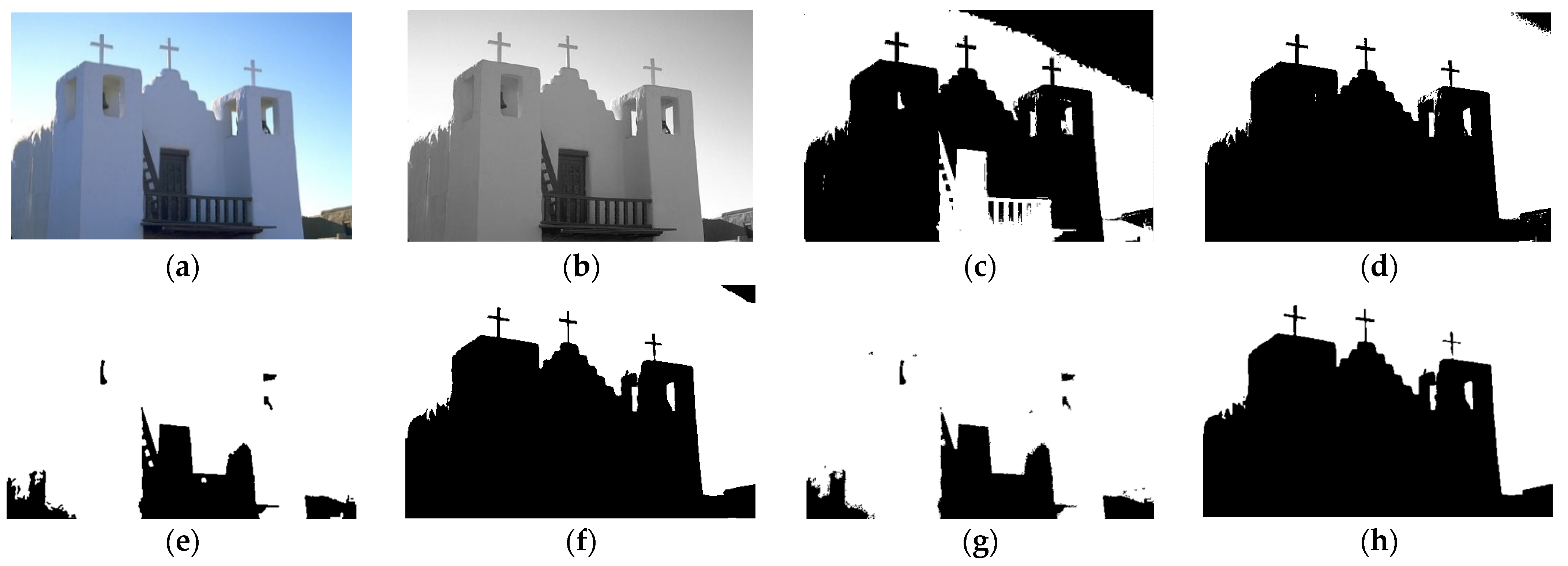
4.1. Segmentation of Building

Building is the main carrier of production and life of human society. Traditional building images are easily affected by illumination and noise in the process of capture. The final image may have texture and corresponding noise. In the first experiment, we select No.24063 image in the BSD500 dataset, which resolution is 481 × 321. The goal is to divide the image into two categories: foreground building and background sky, as shown in Figure 3. Among Figure 3a is the original image, Figure 3b is gray scale image, Figure 3c–h are GMM, FCM, FFCM, FLICM, FRGMM and our method. The upper right corner of the rendering in Figure 3c,d,f reflects some areas that are mistakenly classified as buildings. Among them, the misclassification area of GMM Figure 3c is larger than other methods.

Table 1. PA value of image data. The bold numbers suggest the highest value.

Image ID	GMM	FCM	FFCM	FLICM	FRGMM	Ours
3063	0.8337	0.5587	0.5403	0.5889	0.9912	0.8455
12003	0.6341	0.5266	0.6425	0.6756	0.6518	0.7376
24063	0.5467	0.7216	0.5458	0.7234	0.5483	0.9625
86016	0.9303	0.8354	0.8938	0.9314	0.8338	0.9938
135069	0.6135	0.7162	0.6132	0.9103	0.6124	0.9455
296059	0.8857	0.9005	0.8845	0.8989	0.8275	0.9215
302003	0.6994	0.8405	0.8035	0.8161	0.7884	0.8653
Mean	0.7347	0.7285	0.7033	0.7920	0.7504	0.8959

and

Table 2. Dice value of image data. The bold numbers suggest the highest value.

Image ID	GMM	FCM	FFCM	FLICM	FRGMM	Ours
3063	0.5994	0.4704	0.4197	0.4748	0.9707	0.6776
12003	0.5183	0.5266	0.5291	0.5465	0.5504	0.6497
24063	0.5688	0.5320	0.5670	0.5371	0.5726	0.6142
86016	0.8174	0.7153	0.7812	0.8256	0.6478	0.8339
135069	0.2246	0.6036	0.2245	0.9192	0.2255	0.9920
296059	0.8291	0.8402	0.8234	0.8311	0.8183	0.9176
302003	0.6637	0.7124	0.6585	0.7446	0.7358	0.7561
Mean	0.6030	0.6286	0.5719	0.6969	0.6458	0.7773

shows the two objective indices for the matching between the rendering of the image and the benchmark image. It can be seen that the segmentation accuracy of the proposed method is the highest, and the PA value of our proposed method is 0.9625. From an objective point of view, the segmentation effect of the proposed method for the building image is better, and it reflects more detailed features section, such as the two upper right windows in Figure 3h and the details. Therefore, whether from the subjective or objective point of view, it can be concluded that the proposed method has a good segmentation effect on the building image, which can not only segment accurately, but also retain the image details for image analysis.

4.2. Segmentation of Human Face

In the second experiment, human face is selected to segment, which is No.302003 in Berkeley dataset and its resolution is 321 × 481. The target is to divide the image into two categories, foreground face and another is background. The original shown in Figure 4a,b is gray scale. Figure 4c–h are the segmentation result diagrams after processing the image by several methods. As shown in Figure 4, we can see that the eyebrows in the upper left corner of Figure 4c have been lost. In Figure 4h, the specific details of the face and the expression and details of the eyebrows of the two eyes are shown. Other methods such as FFCM Figure 4e not only lose the eyebrow details, but also the background has been misclassified. In addition, our method not only can segment the facial information perfectly, achieves the expected segmentation effect, but also reflect the texture details of eyebrows and sleeves. Table 1 and Table 2 gives the experimental calculation values of several methods on No.302003.

It can be seen from Table 1 that PA = 0.8653 of this method is the maximum value, which shows that the segmentation performance of this method is more accurate than other methods. In addition, the value of dice = 0.07561 is more prominent than the dice parameters of other methods. Compared with other methods, this method can not only achieve the segmentation accuracy, but also reflect the local details of the eyebrows and eyes on the face and the texture details of the sleeves.

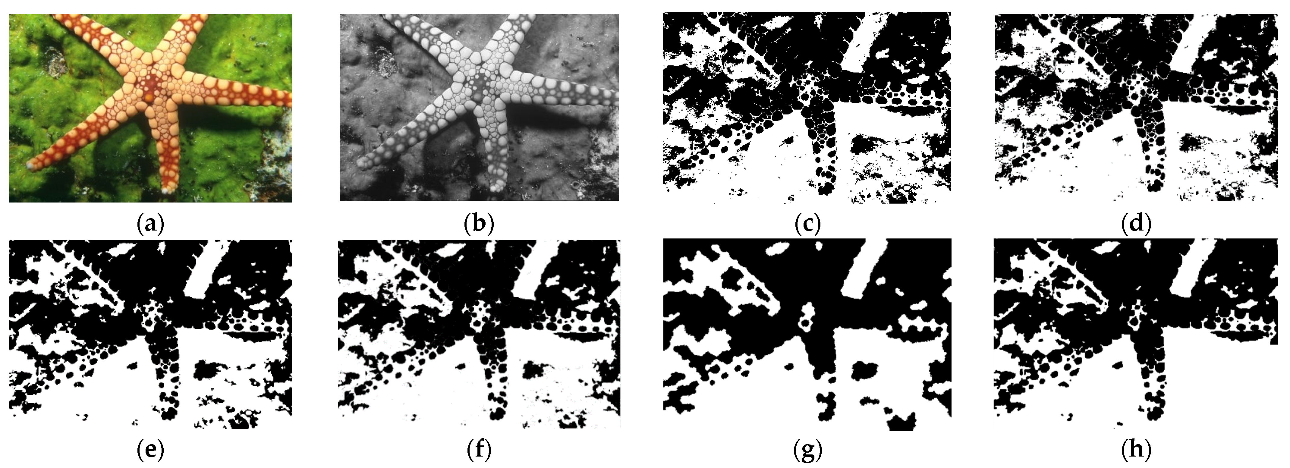
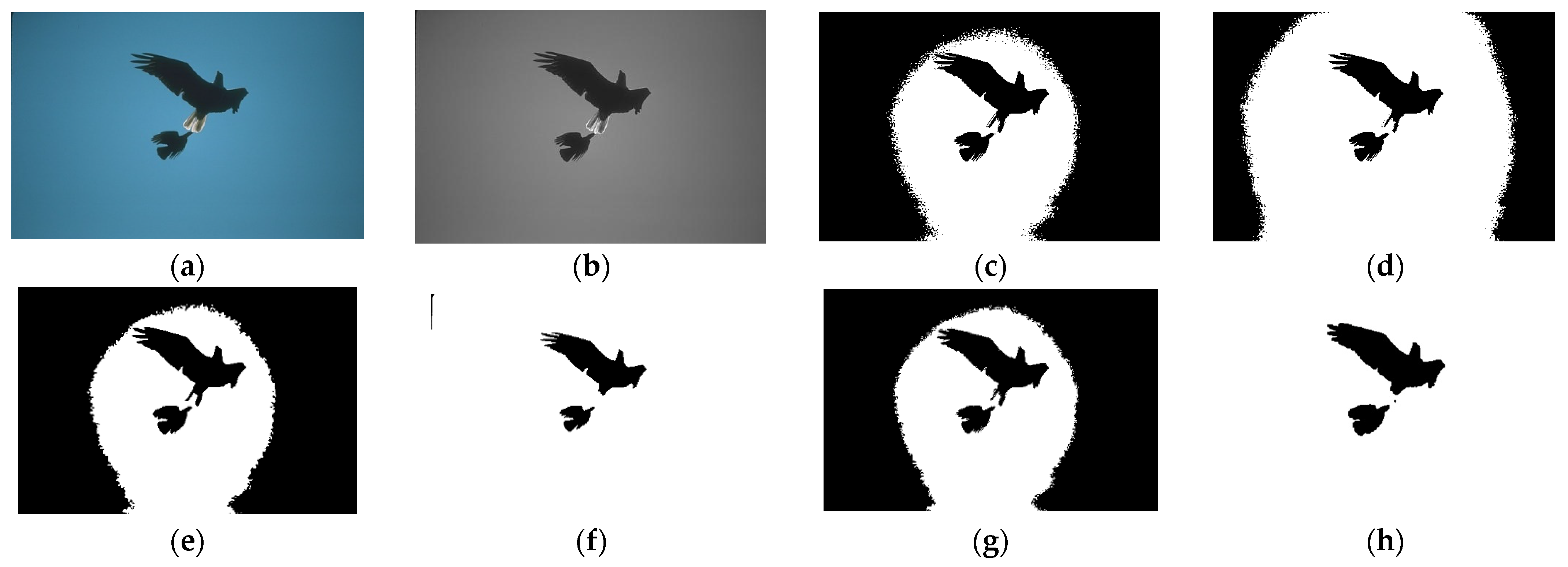
4.3. Segmentation of a Large Target and a Small Background

In the third experiment, we selected a large target, relatively small background image, namely starfish, which is NO.12003 and resolution of 481×321 from the Berkeley datasets. The original image is shown in Figure 5a. Our ultimate goal is to divide it into two categories, starfish and seabed background. Because the image is difficult to distinguish from the seafloor background, the overall effect is not very good when the image is segmented. However, through the comparison of several methods, we can see that the method can be better than other methods when distinguishing starfish from the bottom of the sea. According to Table 1, it can be seen that the PA value of our method is 0.7376 in segmentation accuracy, although not very high, the results are relatively better than the comparison methods, and the dice value in Table 2 is also the maximum among multiple comparison methods.

4.4. Segmentation of a Large Background and a Small Target

In the fourth experiment, we choose a smaller target and a larger background, which is from the Berkeley dataset No. 135069. The original image is shown in Figure 6a. There are two eagles flying in the original image. Therefore, our segmentation goal is to divide the original image into two categories, namely, the eagle is one category, and the sky is the background. Figure 6c–h are the contrast method and ours in this paper. In Figure 6c,d,e,g, we can see that the eagle and part of the sky are divided into a category, the sky is mistakenly divided into foreground and the misclassification area is large. However, in the FLICM Figure 6f there is still a small range of background misclassification in the upper left corner. But this method can classify the sky and hawks completely.

As can be seen from Table 1, the PA value of our method is 0.9455, and the dice value is 0.9920, both of which are the highest. Therefore, the proposed method has a good effect on the small target image segmentation.

4.5. Segmentation of a Medical Image

In the fifth experiment of this paper, we choose the brain image, which is from Brain Web: Simulated MRI Volumes for a normal Brain. The relevant parameters of the data are T1 Modality, which slice thickness is 1 mm and the level of noise has seven levels: 0%, 1%, 3%, 5%, 7% and 9%. Here is 9%. Intensity non-uniformity has three levels: 0%, 20% and 40%. The original image is shown in Figure 7a, namely N9F40, which noise is 9% and intensity non-uniformity is 40%.

The PA value of FTGMM (ours) is the highest value in those methods. We can see from Figure 7 that the brain image segmentation performance of this paper is the best for noisy images. The gray area represents gray matter, the white area represents white matter and the black area represents background and cerebrospinal fluid. The effect image Figure 7h segmented by this method has the best robustness. Therefore, this method has a good segmentation performance in the brain map of a medical image.

Through the segmentation comparison of several groups of images, we can see that the proposed method performs better in practical application. This is not only reflected in the subjective vision, but also reflected in the objective evaluation index. Table 1 and Table 2 objectively show the segmentation accuracy. In addition, we also calculate the comprehensive average of these data. The average segmentation accuracy PA value of the proposed method is 0.8959, and the average dice value is 0.7773. Both data show that the proposed method is more accurate and robust.

5. Conclusions

In this paper, an improved algorithm is proposed and implemented. In the traditional Gaussian mixture model (GMM), the mechanism of visual attention in the field of computer vision is added, namely, saliency map. The value of saliency map is used as neighborhood information of current pixel points by the frequency-tuned salient detection algorithm, which is introduced into GMM in a way of spatial information weight. The salient weight of the pixel strengthens the importance of the point of the image and assists the model in the classification of pixels. Besides, the method based on frequency tuning can be processed independently; thus, the implementation of the whole model is simpler and faster. In addition, the EM algorithm is mature, so it can be easily solved. All experimental data in this paper are presented by Berkeley dataset and Brain Web. Through a visual graph and numerical objective display of various evaluation indexes, we can draw the following conclusion: our method is better than the five methods mentioned in this paper and has good performance for different scene categories. Our method presented in this paper has proven to be simple and has good performance on accurate segmentation, what’s more, reflecting local details to a certain extent and the robustness of the proposed algorithm is better.

References

1. Gemme, L.; Dellepiane, S.G. An automatic data-driven method for SAR image segmentation in sea surface analysis. IEEE Trans. Geosci. Remote Sens. 2018, 56, 2633–2646. [Google Scholar] [CrossRef]
2. Guo, Y.; Jiao, L.; Wang, S.; Wang, S.; Liu, F.; Hua, W. Fuzzy-superpixels for polarimetric SAR images classification. IEEE Trans. Fuzzy Syst. 2018, 26, 2846–2860. [Google Scholar] [CrossRef]
3. Rahman, A.; Verma, B.; Stockwell, D. An hierarchical approach towards road image segmentation. In Proceedings of the 2012 International Joint Conference on Neural Networks (IJCNN), Brisbane, QLD, Australia, 10–15 June 2012; pp. 1–8. [Google Scholar]
4. Soh, S.S.; Tan, T.S.; Alang, T.A.I.T.; Supriyanto, E. White matter hyperintensity segmentation on T2 FLAIR brain images using supervised segmentation method. In Proceedings of the 2016 International Conference on Robotics, Automation and Sciences (ICORAS), Ayer Keroh, Melaka, Malaysia, 5–6 November 2016; pp. 1–3. [Google Scholar]
5. Khaizi, A.S.A.; Rosidi, R.A.M.; Gan, H.-S.; Sayuti, K.A. A mini review on the design of interactive tool for medical image segmentation. In Proceedings of the 2017 International Conference on Engineering Technology and Technopreneurship (ICE2T), Kuala Lumpur, Malaysia, 18–20 September 2017; pp. 1–5. [Google Scholar]
6. Hameed, K.; Chai, D.; Rassau, A. Score-based mask edge improvement of Mask-RCNN for segmentation of fruit and vegetables. Expert Syst. Appl. 2022, 190, 116205. [Google Scholar] [CrossRef]
7. Geng, X.; Zhou, Z.-H.; Smith-Miles, K. Individual Stable Space: An Approach to Face Recognition under Uncontrolled Conditions. IEEE Trans. Neural Netw. 2008, 19, 1354–1368. [Google Scholar] [CrossRef] [PubMed] [Green Version]
8. Zhang, G.; He, L.; Zhang, T. A security scheme based on time division multiplex. In Proceedings of the 2011 Cross Strait Quad-Regional Radio Science and Wireless Technology Conference, Harbin, China, 26–30 July 2011; pp. 1172–1174. [Google Scholar]
9. Yang, H. Research on Thresholding Methods for Image Segmentation. J. Liaoning Univ. 2006, 33, 135–137. [Google Scholar]
10. Fan, J.; Yau, D.; Elmagarmid, A.; Aref, W. Automatic Image Segmentation by Integrating Color-Edge Extraction and Seeded Region Growing. IEEE Trans. Image Processing 2001, 10, 1454–1466. [Google Scholar]
11. Fernandez-Maloigne, C.; Robert-Inacio, F.; Macaire, L. Region Segmentation; John Wiley & Sons, Ltd.: Hoboken, NJ, USA, 2013. [Google Scholar]
12. Pearson, K. Contributions to the Mathematical Theory of Evolution. Philos. Trans. R. Soc. Lond. A 1894, 185, 71–110. [Google Scholar]
13. Moon, T.K. The expectation-maximization algorithm. IEEE Signal Processing Mag. 1996, 13, 47–60. [Google Scholar] [CrossRef]
14. Dempster, A.P.; Laird, N.M.; Rubin, D.B. Maximum likelihood from incomplete data via the EM algorithm. J. R. Stat. Soc. Ser. B Methodol. 1977, 39, 1–38. [Google Scholar]
15. Bilmes, J.A. A gentle tutorial of the EM algorithm and its application to parameter estimation for Gaussian mixture and hidden Markov models. Int. Comput. Sci. Inst. 1998, 4, 126. [Google Scholar]
16. McLachlan, G.; Krishnan, T. The EM Algorithm and Extensions; Wiley: New York, NY, USA, 2007; Volume 382. [Google Scholar]
17. Acito, N.; Corsini, G.; Diani, M. An unsupervised algorithm for hyperspectral image segmentation based on the Gaussian mixture model. In Proceedings of the 2003 IEEE International Geoscience and Remote Sensing Symposium, Toulouse, France, 21–25 July 2003; Volume 6, pp. 3745–3747. [Google Scholar]
18. Diplaros, A.; Vlassis, N.; Gevers, T. A Spatially Constrained Generative Model and an EM Algorithm for Image Segmentation. IEEE Trans. Neural Netw. 2007, 18, 798–808. [Google Scholar] [CrossRef] [PubMed] [Green Version]
19. Zhang, H.; Wu, Q.M.J.; Nguyen, T.M. Nguyen. Incorporating Mean Template into Finite Mixture Model for Image Segmentation. IEEE Trans. Neural Netw. Learn. Syst. 2013, 24, 328–335. [Google Scholar] [CrossRef]
20. Chen, L.; Qiao, Y. Markov random field based dynamic texture segmentation using inter-scale context. In Proceedings of the 2016 IEEE International Conference on Information and Automation (ICIA), Ningbo, China, 1–3 August 2016; pp. 1924–1927. [Google Scholar]
21. Courbot, J.-B.; Mazet, V. Pairwise and Hidden Markov Random Fields in Image Segmentation. In Proceedings of the 2020 28th European Signal Processing Conference (EUSIPCO), Amsterdam, The Netherlands, 18–21 January 2021; pp. 2458–2462. [Google Scholar]
22. He, H.; Lu, K.; Lv, B. Gaussian Mixture Model with Markov Random Field for MR Image Segmentation. In Proceedings of the 2006 IEEE International Conference on Industrial Technology, Mumbai, India, 15–17 December 2006; pp. 1166–1170. [Google Scholar]
23. Liu, X.-Y.; Liao, Z.-W.; Wang, Z.-S.; Chen, W.-F. Gaussian Mixture Models Clustering using Markov Random Field for Multispectral Remote Sensing Images. In Proceedings of the 2006 International Conference on Machine Learning and Cybernetics, Dalian, China, 13–16 August 2006; pp. 4155–4159. [Google Scholar]
24. Tang, H.; Dillenseger, J.L.; Bao, X.D.; Luo, L.M. A vectorial image soft segmentation method based on neighborhood weighted Gaussian mixture model. Comput. Med. Imaging Graph. 2009, 33, 644–650. [Google Scholar] [CrossRef] [Green Version]
25. Zhang, R.; Ye, D.H.; Pal, D.; Thibault, J.-B.; Sauer, K.D.; Bouman, C.A. A Gaussian Mixture MRF for Model-Based Iterative Reconstruction with Applications to Low-Dose X-Ray CT. IEEE Trans. Comput. Imaging 2016, 2, 359–374. [Google Scholar] [CrossRef] [Green Version]
26. Oliver, G.; Klaus, T. Subject-Specific Prior Shape Knowledge in Feature-Oriented Probability Maps for Fully Automatized Liver Segmentation in MR Volume Data. Pattern Recognit. 2018, 84, 288–300. [Google Scholar]
27. Asheri, H.; Hosseini, R.; Araabi, B.N. A New EM Algorithm for Flexibly Tied GMMs with Large Number of Components. Pattern Recognit. 2021, 23, 107836. [Google Scholar] [CrossRef]
28. Bi, H.; Tang, H.; Yang, G.; Shu, H.; Dillenseger, J.-L. Accurate image segmentation using Gaussian mixture model with saliency map. Pattern Anal. Appl. 2018, 21, 869–878. [Google Scholar] [CrossRef] [Green Version]
29. Hou, X.; Zhang, L. Saliency detection: A spectral residual approach. In Proceedings of the 2007 IEEE Conference on Computer Vision and Pattern Recognition, Minneapolis, MN, USA, 17–22 June 2007; pp. 1–8. [Google Scholar]
30. Itti, L.; Koch, C.; Niebur, E. A model of saliency-based visual attention for rapid scene analysis. Proc. IEEE Trans. Pattern Anal. Mach. Intell. 1998, 20, 1254–1259. [Google Scholar] [CrossRef] [Green Version]
31. Borji, A.; Itti, L. State-of-the-art in visual attention modeling. IEEE Trans. Pattern Anal. Mach. Intell. 2013, 35, 185–207. [Google Scholar] [CrossRef]
32. Walther, D.; Itti, L.; Riesenhuber, M.; Poggio, T.; Koch, C. Attentional selection for object recognition—A gentle way. In International Workshop on Biologically Motivated Computer Vision; Springer: Berlin/Heidelberg, Germany, 2002; pp. 472–479. [Google Scholar]
33. Achanta, R.; Hemami, S.; Estrada, F.; Susstrunk, S. Frequency-tuned salient region detection. In Proceedings of the 2009 IEEE Conference on Computer Vision and Pattern Recognition, Miami, FL, USA, 20–25 June 2009; pp. 1597–1604. [Google Scholar]
34. Blekas, K.; Likas, A.; Galatsanos, N.P.; Lagaris, I.E. A spatially constrained mixture model for image segmentation. IEEE Trans. Neural Netw. 2005, 16, 494–498. [Google Scholar] [CrossRef]
35. Guo, Y.; Zi, Y.; Jiang, Y. Contrastive Study of Distributed Multitask Fuzzy C-means Clustering and Traditional Clustering Algorithms. In Proceedings of the 2020 5th International Conference on Communication, Image and Signal Processing (CCISP), Chengdu, China, 13–15 November 2020; pp. 239–245. [Google Scholar]
36. Nguyen, T.M.; Wu, Q.M. A fuzzy logic model based on Markov random field for medical image segmentation. Evol. Syst. 2013, 4, 171–181. [Google Scholar] [CrossRef]
37. Krinidis, S.; Chatzis, V. A robust fuzzy local information C-means clustering algorithm. IEEE Trans. Image Process. 2010, 19, 1328–1337. [Google Scholar] [CrossRef] [PubMed]
38. Nguyen, T.M.; Wu, Q.M.J. Fast and robust spatially constrained Gaussian mixture model for image segmentation. IEEE Trans. Circuits Syst. Video Technol. 2013, 23, 621–635. [Google Scholar] [CrossRef]
39. Martin, D.; Fowlkes, C.; Tal, D.; Malik, J. A database of human segmented natural images and its application to evaluating segmentation algorithms and measuring ecological statistics. In Proceedings of the 8th IEEE International Conference on Computer Vision, Vancouver, BC, Canada, 7–14 July 2001; pp. 416–423. [Google Scholar]
Figure 1. Difference between the traditional GMM and the proposed method.
Information 13 00098 g001
Figure 2. Extraction of saliency map by frequency-tuned salient detection.
Information 13 00098 g002
Figure 3. Segmentation of the building. (a) Original, (b) gray scale, (c) GMM, (d) FCM, (e) FFCM, (f) FLICM, (g) FRGMM and (h) ours.
Information 13 00098 g003
Figure 4. Segmentation of the human face. (a) Original, (b) gray scale, (c) GMM, (d) FCM, (e) FFCM, (f) FLICM, (g) FRGMM and (h) ours. (Adapted from Berkeley dataset, 302003).
Information 13 00098 g004
Figure 5. Segmentation of a large object and a small background. (a) Original, (b) gray scale, (c) GMM, (d) FCM, (e) FFCM, (f) FLICM, (g) FRGMM and (h) ours.
Information 13 00098 g005
Figure 6. Segmentation of a large background and a small target. (a) Original, (b) gray scale, (c) GMM, (d) FCM, (e) FFCM, (f) FLICM, (g) FRGMM and (h) ours.
Information 13 00098 g006
Figure 7. Segmentation of a medical image. (a) Noise image, (b) ground truth, (c) GMM (PA = 0.6964), (d) FCM (PA = 0.7106), (e) FFCM (PA = 0.7001).,(f) FLICM (PA = 0.6233), (g) FRGMM (PA = 0.4857) and(h) ours (PA = 0.7490).
Information 13 00098 g007