Tuberculosis Bacteria Detection and Counting in Fluorescence Microscopy Images Using a Multi-Stage Deep Learning Pipeline

Abstract

The manual observation of sputum smears by fluorescence microscopy for the diagnosis and treatment monitoring of patients with tuberculosis (TB) is a laborious and subjective task. In this work, we introduce an automatic pipeline which employs a novel deep learning-based approach to rapidly detect Mycobacterium tuberculosis (Mtb) organisms in sputum samples and thus quantify the burden of the disease. Fluorescence microscopy images are used as input in a series of networks, which ultimately produces a final count of present bacteria more quickly and consistently than manual analysis by healthcare workers. The pipeline consists of four stages: annotation by cycle-consistent generative adversarial networks (GANs), extraction of salient image patches, classification of the extracted patches, and finally, regression to yield the final bacteria count. We empirically evaluate the individual stages of the pipeline as well as perform a unified evaluation on previously unseen data that were given ground-truth labels by an experienced microscopist. We show that with no human intervention, the pipeline can provide the bacterial count for a sample of images with an error of less than 5%.

1. Introduction

Mycobacterium tuberculosis (Mtb) is the causative microorganism of tuberculosis (TB), one of the leading infectious causes of death worldwide [1]. The pathogen is droplet and aerosol-transmitted, with up to 85% of the disease affecting the lungs [2]. According to WHO, up to 2 billion individuals globally harbour the Mtb bacteria in their body, with up to 10 million cases of active disease and 2 million deaths per year [2]. The greatest burden of morbidity and mortality from TB occurs in low- and middle-income countries, which have fewer healthcare resources [3]. Early TB detection increases a patient’s chance of cure and recovery as well as helps to prevent onward disease transmission [2,4,5].

Traditionally, the main tool for TB diagnosis has been sputum smear microscopy. Sputum samples expectorated by symptomatic patients are heat-fixed onto slides and stained according to laboratory protocols, which label acid-fast bacteria (AFB) such as Mtb cells. The older Ziehl–Neelsen protocol stains AFB red against a blue background for light microscopy (usually at ×1000 magnification), whilst the newer Auramine-based protocols stain them yellow-green against a black background for fluorescence microscopy (usually at ×400 magnification). In order to quantify the bacterial burden within a patient’s lungs, semi-quantitative grading scales have been developed. Sputum smear microscopy results are generally reported as ‘negative’, ‘scanty’, ‘1+’, ‘2+’, or ‘3+’ [6,7].

In recent years, many centres worldwide have shifted their focus away from smear microscopy towards molecular tools (e.g., the Xpert MTB/RIF assay) for TB diagnosis [8]. However, sputum smear gradings remain useful for the triaging of disease severity and prognosis, with possible implications for the individualization of therapy [9] and the monitoring of treatment response where molecular tests are currently not recommended [2].

Researchers who study the metabolic adaptation of M. tuberculosis to drug pressure and other physiological stresses are also interested in the microscopic appearances of individual bacterial cells. Changes in the length and width of cells [10], loss of acid fastness [11], and accumulation of intracellular lipid [11,12,13] may influence the transmissibility and antibiotic tolerance of M. tuberculosis. Microscopy remains an important tool for the description and investigation of these features.

In clinical microbiology practice, smear microscopy delivers results much more quickly than waiting for Mtb to grow in culture [6]. When performed well, it has high specificity (99%) in the identification of Mtb cells [7]. Switching from traditional Ziehl–Neelsen to fluorescence Auramine-based microscopy has increased the sensitivity of smear microscopy (from 0.34–0.94 to 0.52–0.97 according to one systematic review) [14,15]. Indeed, as shown, amongst others, by Zou et al. [16], Mtb bacteria are more easily differentiated from their surroundings when fluorescence microscopy is used rather than conventional microscopy; see Figure 1. There are, however, challenges to the effective use of microscopy for clinical patient management and the academic study of Mtb.

Although laboratory consumables for microscopy are generally inexpensive, the procedure is time-consuming, which creates cost implications for laboratory staffing. The wide range of diagnostic sensitivity that are reported for TB smear microscopy also reflect the difficulty and subjectivity associated with performing the technique.

Retaining a high level of proficiency as a microscopist requires a regular investment of time. General guidelines recommend that practitioners must examine at least 25 slides per day to remain competent [6]. Each slide is divided into smaller microscopic fields which are analysed one-by-one, and it is inevitable that human error and fatigue may affect specificity and sensitivity performance [17]. Some slides are difficult to read because some AFB have atypical appearances, and some non-bacterial components (artefacts) within the sputum matrix look similar to Mtb cells and may be mistaken for them.

Many of the aforementioned challenges to manual, that is, human-based analysis of microscopic slides can be addressed by means of modern computer vision and machine learning techniques. Indeed, this is the nature of the key contributions of the present work. More specifically, we introduce herein the following novelties:

• We describe a fast method for extracting a new representation of microscopic slides, which enhances the differentiation of bacteria from their background;
• We describe a novel method for the detection of salient, that is, bacteria-containing regions within microscopic slides, which uses cycle-consistent generative adversarial networks to synthesise slides with bounding box annotations;
• We introduce a transfer learning-trained convolutional neural network-based refinement of the list of salient regions detected in the previous step;
• We propose a convolutional neural network-based method for counting bacteria, which appear in highly variable ways, in image patches, using regression as a means of increasing the robustness of the count.

2. Related Work

Deep learning algorithms utilising convolutional neural networks (CNNs) or deep convolutional neural networks (DCNNs) [18] have been successful in tackling similar bacteria/cell detection in other branches of biomedical science over the last decade. For example, a recent work on neurological tissue, “Find-My-Cells”, employed DCNN to identify astrocytes in brain disorders, with performance equivalent to that of a human specialist [19]. That project also highlighted how an automated neural network might be able to reach more objective decisions across an entire dataset of images because it can view all of the data simultaneously, whilst a human operator can only assess image sections sequentially [19]. Decisions made by the network are also deterministic, which means that consistent results will be obtained from training the network [19]. In contrast, a clinician reviewing the same sample on different occasions may reach different conclusions.

It is difficult to detect and count contacting and overlapping bacilli in sputum, and most of the existing algorithms fail to do so accurately [20]. Indeed, most reliably detect only isolated bacilli. A representative example is the work of Sotaquirá et al. [21], which used conventional bright field microscopy and simple colour thresholding for the localization of bacteria. Their count was rather crudely estimated based on the average bacterial size and the corresponding areas of the detected salient regions. In empirical experiments, this method achieved an error of 14.3%.

A more recent work by Mithra et al. also made use of conventional microscopic images [22]. They, similar to Sotaquirá et al., segmented via colour space transformation and colour thresholding [21,22]. An intermediate step was proposed to categorize segments according to their length, area, density, and appearance histogram properties in order to determine if they contained bacteria or not. Finally, they employed four distinct types of classifiers to determine the number of bacteria in each image. Unfortunately, the method was analysed rather poorly, without any error analysis being reported. In one of the most recently published papers on the topic, Vente et al. proposed a fairly complex method for the localization of bacteria, employing edge detection, Fourier analysis, and morphological operators [12], and thereafter estimating the bacterial count in the regions of interest using simple regression. The authors reported an error of 6.5% in the empirical experiments.

3. Proposed Method

The present section explains the key steps of the proposed algorithm in detail, namely (i) the extraction of an enhanced representation of the input slide, (ii) semantic segmentation of the slide, (iii) salient image patch extraction, and (iv) regression-based inference of the bacterial count from the extracted patches.

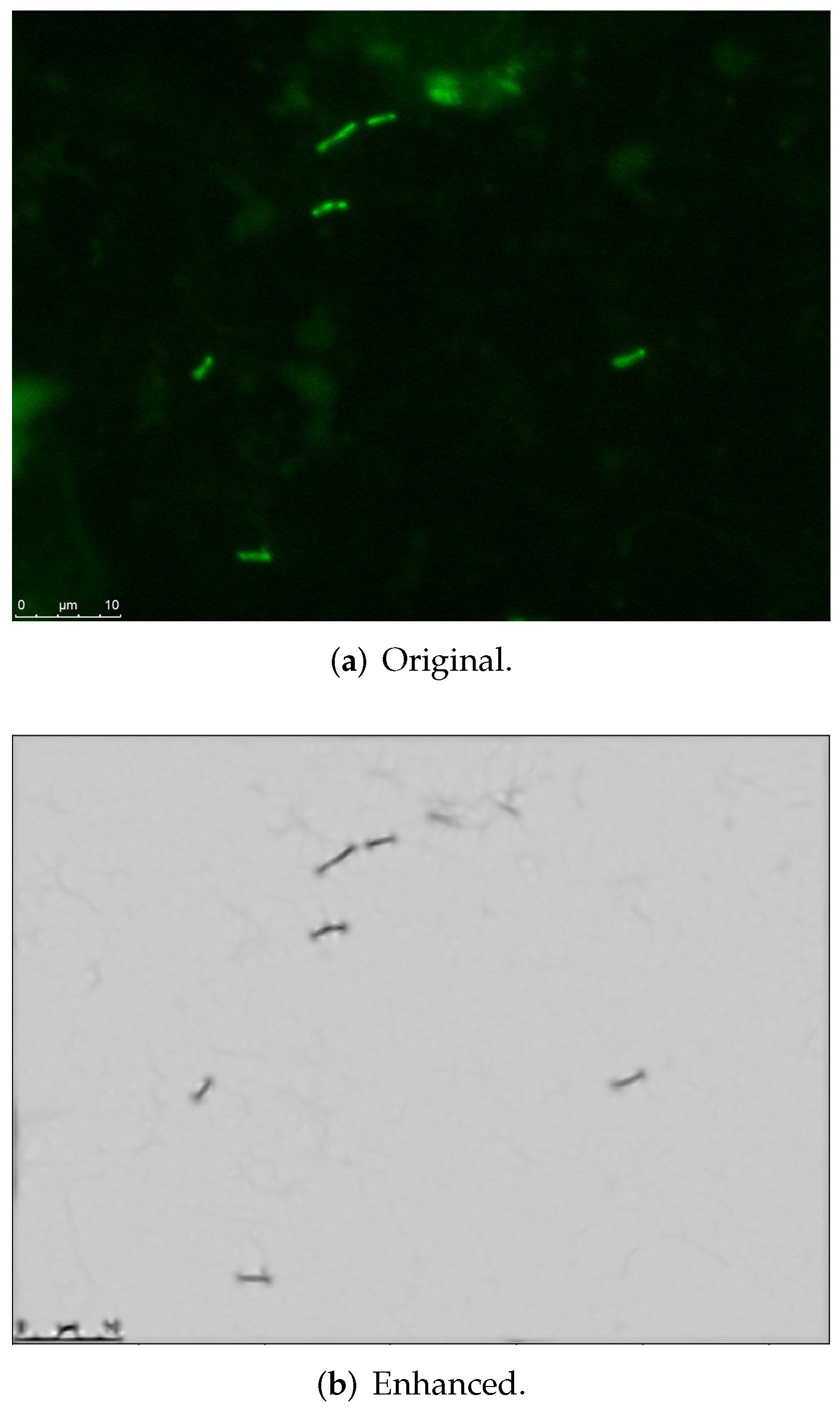
3.1. Image Processing-Based Enhanced Representation Extraction

The ability to create high-quality microscopic images is dependent on the quality of the clinical samples collected and various choices pertaining to the smear preparation and staining. Thick smears from very mucous samples can be associated with excessive background staining, and artefacts may interfere with bacterial identification. Some Mtb cells are less acid-fast than others, particularly during treatment. This may reduce their capacity to retain Auramine-O, reducing the intensity of their fluorescence in comparison to the background and making them harder to identify.

To address the aforementioned issues, amongst others, in the present work, we propose an image processing-based stage as a means of enhancing the image content of interest and suppressing confounding content, including artefacts. Our starting point is the observation that the bacteria of interest is characterized both by its size and shape, namely they form mostly straight, thin, and elongated structures (n.b., this is not the case with all types of bacteria). This observation strongly motivates the use of Hessian-based ridge detection [23]. In particular, the eigendecomposition of the Hessian matrix allows for a differentiation between different kinds of local image behaviour, leading to the straightforward process of distinguishing between blob-like structures, uniform regions, and elongated structures of interest herein. In particular, consider the Hessian matrix with the size of $2\times 2$ pixels, at the scale $\sigma$ and the image locus x:

$$\begin{array}{c}\hfill H=\left[\begin{array}{c}{L}_{xx}(x,\sigma )L_{xy}(x,\sigma )\\ L_{yx}(x,\sigma )L_{yy}(x,\sigma )\end{array}\right]\end{array}$$

(1)

where $L_{xx}(x,\sigma )$ is the convolution of the second-order derivative of a Gaussian $\frac{{\partial }^2}{{\partial }^{2}x}g(x,\sigma )$ with the second derivative of an input image at point x, likewise for $L_{xy}$ and $L_{yy}$ [24,25]. The scale of the Hessian is governed by the value of $\sigma$—the smaller its value, the finer (i.e., more local) the scale, and conversely, the greater its value, the coarser (i.e., more global) the scale. The determination of the value of this parameter can be see as a trade-off emerging from the observation that tuberculosis bacteria in fluorescence images can be distinguished from the remainder of the image content both by its characteristic shape and apparent brightness. In some instances, the shape is less informative, e.g., due to the close packing of different individual bacteria when the brightness becomes the primary cue; similarly, in some instances, the bacteria do not exhibit the expected brightness when it is the shape that becomes the most useful cue. Thus, both aspects of appearance need to be taken into account for maximum robustness, which affects the choice of $\sigma$. The value we used, namely $\sigma =5$, was determined experimentally (compare with other related work [24,25,26]). In principle, when the proposed method is applied on novel data, this value should be adapted to match the scale of bacteria in images and image contrast, which is a matter of simple scaling.

In the proposed method, the computed Hessian matrices across all image loci are next used to extract the pseudo-likelihood of each pixel being incident on a bacterium. Recall that the Hessian is informative regarding the nature of local appearance variation in an image [27]. In particular, considering the bacilli form elongated structures, we are interested in the loci which exhibit significant change in one principal direction (perpendicular to a bacterium) and little change in the other (along a bacterium), and these can be readily identified using the corresponding Hessian matrix eigenvalues [28]. More specifically, to create an enhanced image (in the context of our end goal), each pixel in the original image is replaced with the absolute value of the lower-magnitude value of the Hessian eigenvalue computed at the locus; see Figure 2. The initially appealing alternatives, which take into account both eigenvalues such as the use of the ratio of the two eigenvalues, were found unsuitable due to an increase in noise and dynamic range.

3.2. Semantic Segmentation Using Cycle-Consistent Adversarial Networks

A generative adversarial network (GAN) in its simplest form comprises two CNNs, one referred to as the generator and one as the discriminator, which are trained jointly [29]. Given the data in the input domain, the generator synthesises the data in the target domain [30,31]. On the other hand, the discriminator tries to distinguish between the real data in the target domain and the synthetic data produced by the generator [29,30]. The joint training of the two networks drives the generator to improve its achievement of realism for the synthetically generated data, and the discriminator to become more nuanced in its discrimination. This process can be seen as a competition between two players, each trying to beat the other in a min–max game [32].

A cycle-consistent GAN consists of two complementary GANs and aims to learn domain translation, with the key idea being that each generator learns to synthesise data from the corresponding domain. In our scenario, these two domains are called ‘labelled’ and ‘unlabelled’ smear images. In more detail, using labelled images, one generator learns to synthesise the corresponding unlabelled images, whereas the other uses unlabelled images as input and generates labelled synthetic ones.

Following experimental results reported in previous work [33], we used input image patches with the size of 256 × 256 pixels and additionally re-scaled them to 384 × 384 pixels using bicubic interpolation [34], which was found to effect an improvement in performance. We also introduced alterations to the network architecture by including three further residual blocks as a means of improving the detection of bacteria with lower brightness.

As regards the discriminators, which classify overlapping patches, we adopted an architecture similar to that of the PatchGAN [35,36,37]. However, evidence shows that the relatively large patch size ($70\times 70$ pixels) used by most previous work is unsuitable for the context of tasks in which the generators are trying characteristics that are finer grained and more nuanced in appearance [38]. Hence, we use much smaller $30\times 30$-pixel patches herein instead. Additionally, to further increase the sensitivity and robustness of the model, we introduce a change to the usual number of strides at different layers. In particular, as a means of facilitating the learning in the proximity of the image border, we introduce a reflection pad of size 3.

Table 1. Key parameters of the five-layer discriminators used in the present work. Changes from the usual values used in previous work are shown without highlighting, whereas our task-specific alterations are shown using bold font.

Layer	Kernel Size	Strides	Padding
Layer 1	3 × 3	2	3
Layer 2	3 × 3	1	1
Layer 3	3 × 3	1	1
Layer 4	3 × 3	3	1
Layer 5	3 × 3	2	1

summarizes the key changes.

Training the Cycle-Gan

Here, we summarize the key settings pertaining to the training of our cycle-GAN. To start with, considering the complexity of the learning task at hand, the number of epochs used to train our cycle-GAN was set to 300, which is a considerably higher number than that used in most previous work [33]. Another crucial aspect of training which needs to be correctly determined so as to facilitate successful cycle-GAN learning concerns the learning rates of the generators and discriminators. In particular, a sense of competitive equilibrium has to be maintained between the two kinds of sub-network. If the discriminators are considerably more effective, the network will overfit and the generators’ learning will never converge. Similarly, if generators are more effective, mode collapse is likely, and the desired state of the overall network may never be achieved. Other works that employ cycle-GANs for highly specialised tasks have shown the benefit of differing learning rates for the two sub-networks [38,39]. Similarly, the learning rate of the generators was set to 0.0006 and that of the discriminators to 0.0002. Similar considerations led us to effect a reduction in the (linear) learning rate after 50 epochs—significantly earlier than most other work [33]. We also adopted the use of AdaBelief, a new optimizer which has shown to converge as quickly as adaptive optimizers (such as Adam [40]) and to generalize better than Stochastic Gradient Descent (SGD) [41] in complex architectures such as GANs [42]; see Figure 3. Finally, to maximize the robustness and the generalizability of the learning process, we performed synthetic data augmentation. In particular, we increased the amount of training data by approximately 50% by adding images randomly rotated by $\pm {25}^{\circ }$ and reflected about the vertical or the horizontal axis [43]. Note that this kind of augmentation is particularly principled in the context of the present task because, unlike in the case of natural images wherein there is an inherent asymmetry in directions (e.g., the horizontal and vertical directions are objectively defined and cannot be swapped one for another), in the microscopy slides of interest here, all directions are interchangeable and in that sense equivalent.

3.3. Extracting Salient Patches from Synthetically Labelled Images

Considering that the images based on the enhanced representation described in Section 3.1 are greyscale and the superimposed bounding box red, the localization of the former is a rather straightforward task; see Figure 4. We start by simple colour thresholding, localizing pixels with the red channel value between 150 and 215 (within the range of 0–255), and the green and blue channel values between 90 and 160. The subsequent application of morphological dilation and erosion ensures that the extracted salient structures, which correspond to bounding box contours, are properly closed, thus suppressing the effects of noise.

To further increase the robustness of our approach, we followed the aforementioned low-level processing with a more semantic, domain knowledge-driven refinement. More specifically, guided by the understanding of the size of bacteria in slides, we imposed certain constraints on the extracted bounding boxes. Using the Douglas–Peucker algorithm [44], we first computed a polygonal approximation of imperfectly extracted and possibly overlapping bounded boxes, and then rejected any candidate with a perimeter outside the range of 70–600 pixels. Finally, we extracted the ultimate patches using minimal bounding boxes enveloping the convex hulls of all connected salient structures.

3.4. Classifying Cropped Patches

Heretofore, the aim was to extract as many patches that were of sufficiently bacteria-like appearance by using a rather coarse criterion that facilitates fast processing. As a result, we set the acceptance level relatively low, preferring to capture probable false positives rather than miss them entirely. The goal of the next phase was then to determine whether a selected bacterium patch was a true positive by using more nuanced local appearance. This was challenging because bacteria may overlap, thus greatly increasing the variation in possible appearance. In order to address this variability, we pursued a machine learning approach whereby the discrimination between bacterial and non-bacterial patches was formulated as a classification problem, which was solved using a convolutional neural network. To this end, we applied and compared a number of state-of-the-art models, namely the ResNet family [45], the DenseNet family [46], and the SqueezeNet1_1 family [47]. Each model’s first convolutional layer was replaced with one that consisted of one input channel, one kernel $3\times 3$, one stride 1, and three $3\times 3$ layers. The alterations were motivated by the fact that our slide representation was monochrome (that is, single channel) and the objects of interest were thin, elongated structures that frequently appeared near the image boundary. Every model’s last linear layer was replaced with a single-output linear layer. The linear layer’s output weights were then fed into the sigmoid function. Finally, binary cross entropy was employed as the loss function, and the models were pre-trained on ImageNet.

Approximately 5000 patch images were used for training, with a balanced split between positive and negative examples. Positive examples were extracted using the method explained in Section 3.3, whereas negative ones were selected by randomly sampling from the slides and accepting those patches which did not overlap with any of the positive ones. Approximately 700 images were used for testing. A three-pixel-wide frame was constructed on a randomly chosen positive image (which was known to contain bacteria) to approximate the boundary box formed from the projected labels and to prevent overfitting on the training data. The learning rate was set to 0.0001, with a circular scheduler that had a step size equal to five times the size of the dataset (which in turn was dependent on the batch size) [48]. The base learning rate and the upper learning rate were set to 0.0001 and 0.0002, respectively. Stochastic gradient descent was used as the optimizer since it had been demonstrated to generalize better than Adam [40] in related image classification problems [42]. The model was trained for 100 epochs, with a 0.03 loss and accuracy tolerance, resulting in the termination of training following 20 epochs of no improvement.

3.5. Counting Bacteria

In the final stage of our algorithm, we used regression to infer the number of bacteria present in an input image patch. As we explain in more detail in the next section, we compared a number of different architectures and modified them all by replacing their last linear layer with a single output layer. The mean squared error (MSE) loss function was used for training, and Adam [42,49] was used as the optimizer, with a circular scheduler having the lower and upper boundaries of 0.0001 and 0.00015, respectively; the step size used was equal to twice the size of the dataset. Because patches with more than three bacteria are exceedingly uncommon, we used a relatively low batch size that resulted in a model update following every few examples, thus avoiding the dominance of patches containing a single or two bacteria. Therefore, the batch size was set to 22, or about 5% of the dataset size, in order to maximize the generalizability of the learning.

4. Experimental Evaluation

In this section, we describe an empirical assessment of the proposed algorithm using real-world data. We begin with a description of the data used and follow up with an ablation study of the different stages of our pipeline. Note that the implementation of the proposed method was performed using Pytorch, as were all experiments presented in the present article.

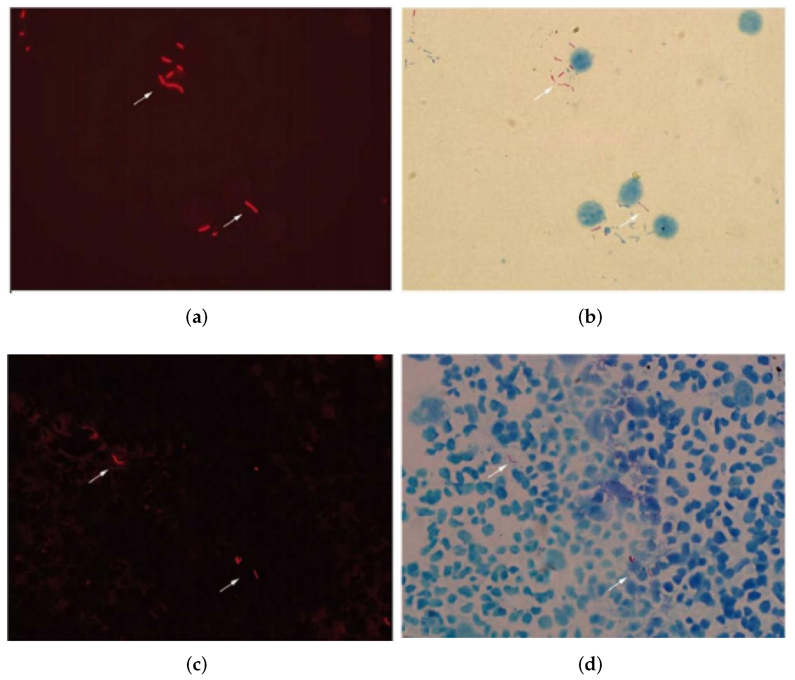
4.1. Data Acquisition

The dataset used in this article comprises microscopic images obtained from a clinical cohort study based in Mbeya, Tanzania, acquired independently, i.e., not specifically for the purpose of the present work. In brief, 46 adults (40 newly and 6 previously diagnosed) with sputum smear-positive pulmonary TB were recruited and followed up until the end of a 6-month course of standard TB treatment, between February 2017 and March 2018. Smears on microscopy slides were prepared from sputum samples collected pre-treatment and at the end of months 2, 4, and 6 of therapy. The slides were stained using the standard Auramine-O method, and the smears were scanned systematically by an experienced microscopist through a fluorescein isothiocyanate filter using a Leica DMLB epifluorescence microscope at ×1000 magnification. All fields containing Auramine-stained, yellow-green AFB were photographed using a digital camera and stored. A total of 230 slides were examined, and 30 images were generated for each AFB-positive slide.

For our experiments, 500 images were selected across all time points of sample collection to ensure that the automated detection and counting networks of Mtb bacteria presented in this work would not be confounded by any changes in the morphology of Mtb cells during or after TB treatment. These images were reviewed within an annotation tool for image labelling by an independent microscopist who had not participated in the original project. Rectangular boxes were superimposed around bacteria within each image and used to tag areas of interest which could contain multiple microorganisms. Overlapping boxes were merged.

4.2. Results

To facilitate an in-depth, nuanced understanding of each stage in the proposed pipeline we performed an ablation study; that is, we evaluated each stage of our algorithm in turns and discussed its contribution to the overall performance [50].

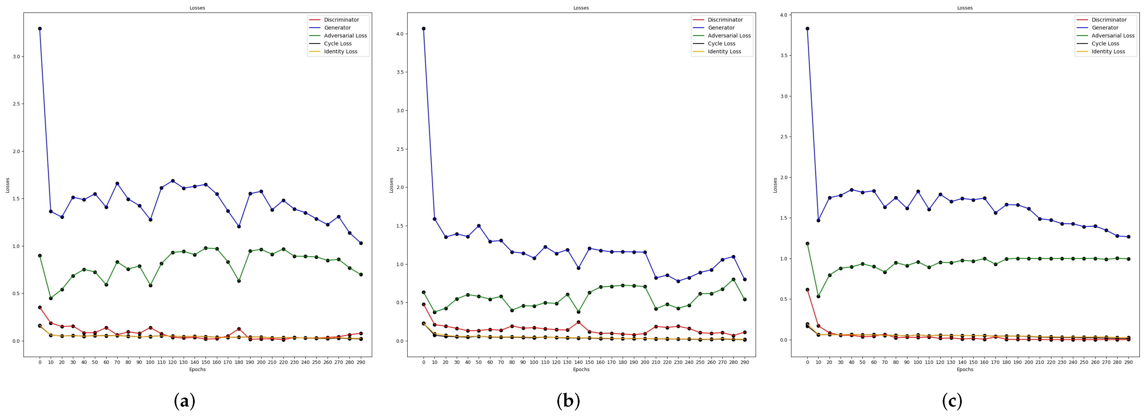
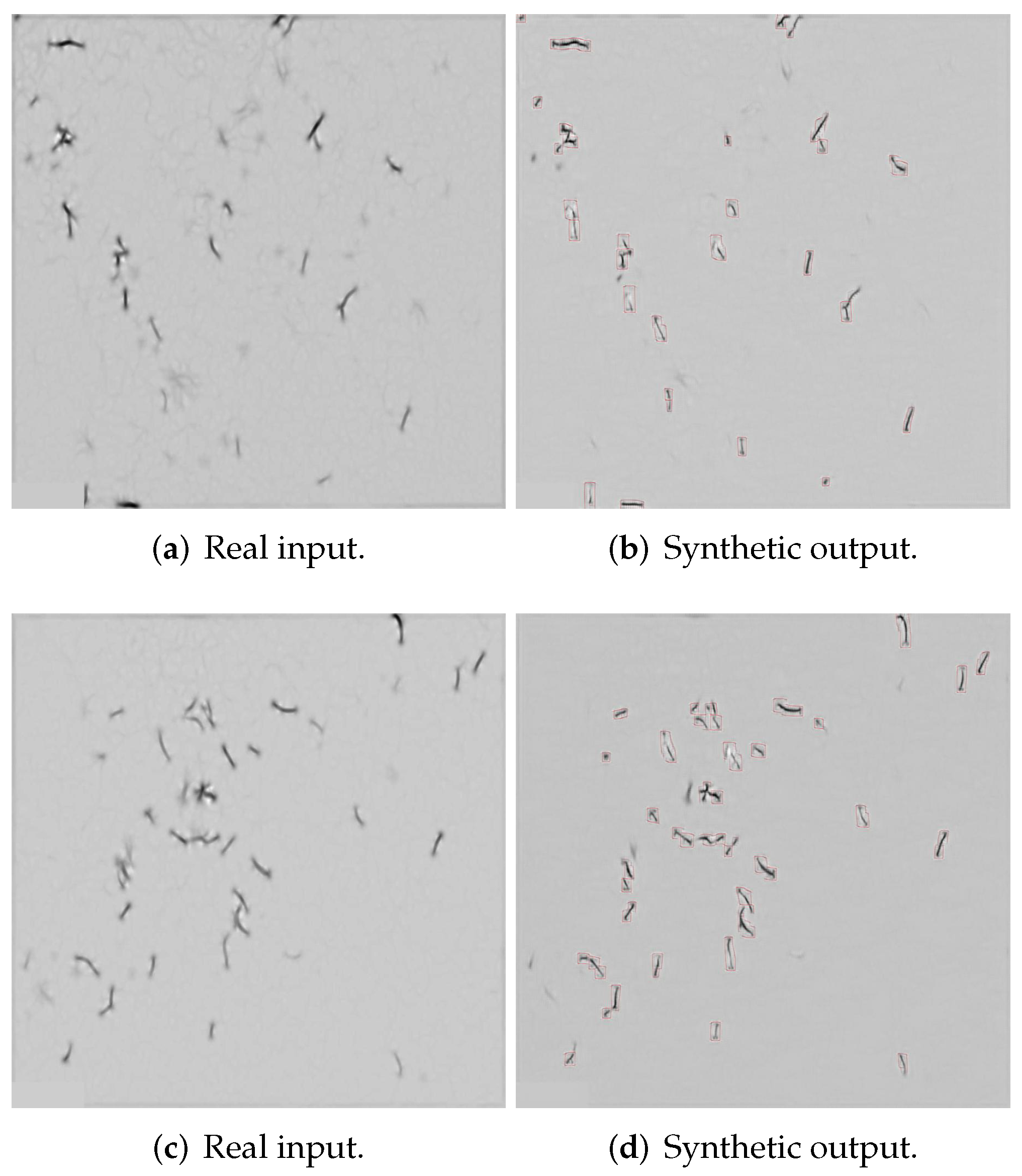
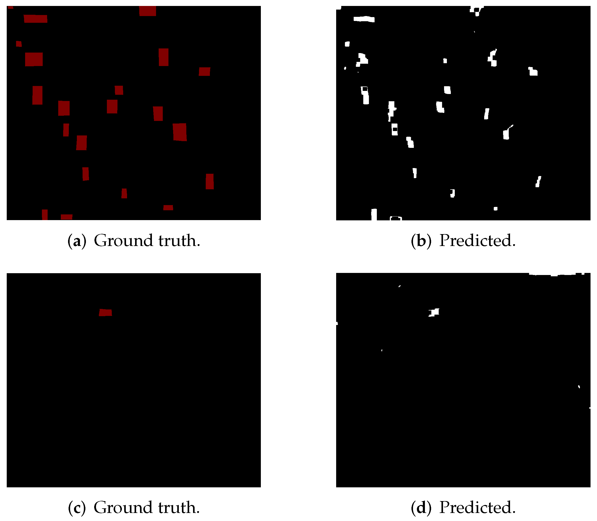
4.2.1. Semantic Segmentation Using Cycle-Gan

To gain insight into the performance of our semantic segmentation, we examined the overlap between ground truth segmentation and that achieved using our automatic method. In other words, we were interested in quantifying the degree of coincidence between two binary images, each comprising regions of interest and the remaining image content, as illustrated in Figure 5.

We started by looking at the usual metrics for this kind of assessment, namely the Jaccard index (also sometimes referred to as the intersection over union, IoU) [51] and the dice coefficient [52]. On our test set, we found these to be 94% and 89%, respectively, suggesting highly effective performance. Indeed, after examining the data manually, we found that the slight deviation from perfect performance was due to boundary effects, which is the slight misalignment of the exact boundaries between the ground truth and the predicted regions of interest rather than an entirely mistaken focus.

To test the aforementioned anecdotal observation, we next introduced a custom performance metric, designed specifically for the task at hand. In particular, we devised a way of deeming each detected salient region as correct or not, allowing us to quantify the number of false positives and false negatives, as well as the distance (error) between each true positive and the corresponding ground truth. To do this, we computed the centroid of each predicted salient region, and if possible, coupled it with the centroid of a ground truth salient region. To determine the pairing, the Euclidean distance between each predicted centroid and all ground truth centroids was calculated, and the nearest one was selected as the correct one. A distance threshold of 35 pixels was also used to reject the coupling of centroids that were excessively far apart. Unpaired predicted regions were considered as false positives. Similarly, unpaired ground truth centroids were considered as false negatives.

Out of 294 ground truth centroids, 3 were not paired, and out of 331 labelled predictions, 40 were not paired. The $L_1$, $L_2$, and $L_{inf}$ distances between paired centroids were found to be 31.49, 13.82, and 10.19 pixels, respectively. Considering that the average width of a single bacillus was between 50 and 120 pixels, these numbers corroborated our previous observation that our segmentation was highly successful, and that the errors suggested by the Jaccard index were mostly due to small misalignments between the predicted and ground truth salient regions. Such errors had little effect on the performance of the entire pipeline as they did not change the actual bacterial count in the patches passed for further processing.

4.2.2. Deep Learning-Based Patch Classification

We next turn our attention to the analysis of the second stage of our algorithm, namely the more nuanced, deep learning-based classification of candidate patches as bacteria-containing ones and those void of bacterial content. Used as the baseline model, we compared a wide range of different architectures, namely ResNet [45], DenseNet [46], and SqueezNet [47], all modified as per Section 3.4. Following training and validation, we evaluated only the model on the test set that came out on top during the validation.

During training, all models reached 100% accuracy; see Figure 6. Greater differentiation was observed during validation, with ResNet50 achieving the highest accuracy of 99.74%, see

Table 2. Validation accuracy achieved by different models. Bold font is used to highlight the best performance according to different criteria (columns).

Model	Accuracy	Precision	Recall	F1-Score
ResNet18	97.28%	0.974	0.949	0.961
ResNet34	99.35%	0.970	0.951	0.960
ResNet50	99.74%	0.990	0.967	0.960
ResNet101	99.61%	0.983	0.958	0.970
ResNet152	99.48%	0.980	0.954	0.967
DenseNet121	95.20%	0.952	0.928	0.939
DenseNet169	88.41%	0.900	0.849	0.874
SqueezeNet	99.38%	0.980	0.958	0.969

. Other ResNet models also performed well, as did SqueezeNet, with the exception of the shallowest ResNet18. Both DenseNet models were significantly worse, and interestingly, the deeper DenseNet169 in particular. In fact, we found that deeper models performed worse, with the validation accuracy decreasing together with the network depth.

Having been identified as the best performing model during validation, we henceforth adopted ResNet50 as the classifier to evaluate the test set. In summary, we found that the proposed machine learning-based filtering increased the overall sensitivity of the pipeline in the discrimination between bacteria-containing patches and those void of bacteria, from 89% attained at the previous, coarse filtering stage, to 97%. Similarly, specificity was increased to 99%, which, to the best of our knowledge, exceeded the performance of all previous work and thus became the new state of the art [53,54,55,56,57].

4.3. Bacterial Count

The final stage of our algorithmic pipeline, and the ultimate nexus, concerns the counting of bacteria in the patches identified as containing bacteria by the preceding stages. Recall that our approach uses regression analysis, thus predicting a real number, although the actual count can only possibly be an integer. This decision was motivated by the desire to retain information about the uncertainty involved in inferring the bacterial count. Thus, the predicted pseudo-count of 1.05 can be interpreted as more confidently corresponding to a single bacterium than, say, 1.48 (whereas 1.51 would tilt the decision towards the count of 2). Our approach also allows for the cancellation of uncorrelated errors across the slide, as observed in previous research [12].

A summary of our experimental results is shown in

Table 3. Performance statistics on unseen test data (second column), and training statistics (columns 3–5). Observe that the more flexible, deeper models tend to overfit and thus perform less well on novel data. This is demonstrated by the training R${}^2$ metric, which is low for these models.

Model	Test Count (Ground Truth $=377$)	MSE	Training MAE	R${}^2$
ResNet18	394	0.0054	0.0345	0.006439
ResNet34	407	0.0444	0.0457	0.006506
ResNet50	414	0.0457	0.0425	0.006523
ResNet101	431	0.0253	0.0236	0.000656
ResNet152	496	0.0231	0.0201	0.000095
DenseNet121	575	0.0104	0.0603	0.000345
DenseNet169	667	0.0086	0.0406	0.000356
SqueezeNet1_1	404	0.0082	0.0227	0.006571

. The best performance was obtained using the simplest and shallowest model, namely ResNet18. Its error of less than 5% is a significant improvement on all previous work, therefore we likewise note here the attainment of the new state of the art [12,21,22]. The visualizations shown in Figure 7 provide further insight into the learning achieved using ResNet18. Both the activation maps and the ultimate count predictions confirm that the network is correctly capturing salient content and appropriately utilizing it to form the ultimate prediction.

Interestingly, note that all models in Table 3 overestimate the bacterial count (the aforementioned ResNet18 the least so). To understand why this is the case, in addition to the ultimate assessment criterion, which is the accuracy of the final count, we include in the table three additional metrics computed during training, namely the mean squared error (MSE), the mean absolute error (MAE), and the coefficient of determination (R${}^2$). Indeed, an examination of the last of these suggests that overly flexible models, which are very deep models with higher numbers of free parameters, overfit during training.

5. Conclusions

Although sputum smear microscopy is being replaced by Xpert MTB/RIF and other molecular assays in many settings worldwide, it still retains a role for some aspects of disease severity assessment and treatment monitoring. The microscopic evaluation of Mtb cells remains important as a research tool. Improved, automated tools to standardize and accelerate image analysis will be beneficial. We have demonstrated how our approach can detect bacilli with a range of morphologies, unlike previous methods which assume a much more uniform appearance [21,22,54,55]. Additionally, unlike existing methods in the literature, our algorithm is capable of correctly counting bacteria near the image border while also exhibiting greater robustness in challenging conditions, owing to the probabilistic nature of the inference at its crux.

Moving forward from these encouraging results, our future work will focus on the extension of the proposed method for the analysis of Mtb bacteria in different growth conditions and under drug pressure. This will include the quantification of the development of intracellular lipid bodies, or the loss of acid-fastness staining characteristics [10,13]. Considering that the proposed method still requires manual microscopy to generate ‘field of interest’ images from stained slides, which is a laborious task, our future work will also include the automation of the image collection process.

References

1. Daley, C.L. The global fight against tuberculosis. Thorac. Surg. Clin. 2019, 29, 19–25. [Google Scholar] [CrossRef] [PubMed]
2. World Health Organization. Global Tuberculosis Report; Technical Report; World Health Organization: Geneva, Switzerland, 2018. [Google Scholar]
3. Zignol, M.; Cabibbe, A.M.; Dean, A.S.; Glaziou, P.; Alikhanova, N.; Ama, C.; Andres, S.; Barbova, A.; Borbe-Reyes, A.; Chin, D.P. Genetic sequencing for surveillance of drug resistance in tuberculosis in highly endemic countries: A multi-country population-based surveillance study. Lancet Infect. Dis. 2018, 18, 675–683. [Google Scholar] [CrossRef]
4. Gele, A.A.; Bjune, G.; Abebe, F. Pastoralism and delay in diagnosis of TB in Ethiopia. Lancet Infect. Dis. 2009, 9, 1–7. [Google Scholar] [CrossRef] [PubMed] [Green Version]
5. Peter, J.G.; van Zyl-Smit, R.N.; Denkinger, C.M.; Pai, M. Diagnosis of TB: State of the art. Eur. Respir. Monogr. 2012, 58, 123–143. [Google Scholar]
6. Hailemariam, M.; Azerefegne, E. Evaluation of Laboratory Professionals on AFB Smear Reading at Hawassa District Health Institutions, Southern Ethiopia. Int. J. Res. Stud. Microbiol. Biotechnol. 2018, 4, 12–19. [Google Scholar]
7. Lin, P.L.; Flynn, J.L. The end of the binary era: Revisiting the spectrum of tuberculosis. J. Immunol. 2018, 201, 2541–2548. [Google Scholar] [CrossRef] [Green Version]
8. Mehta, P.K.; Raj, A.; Singh, N.; Khuller, G.K. Diagnosis of extrapulmonary tuberculosis by PCR. FEMS Immunol. Med. Microbiol. 2012, 66, 20–36. [Google Scholar] [CrossRef] [Green Version]
9. Toman, K. Toman’s Tuberculosis: Case Detection, Treatment and Monitoring. Questions and Answers; World Health Organization: Geneva, Switzerland, 2004. [Google Scholar]
10. Aldridge, B.B.; Fernandez-Suarez, M.; Heller, D.; Ambravaneswaran, V.; Irimia, D.; Toner, M.; Fortune, S.M. Asymmetry and Aging of Mycobacterial Cells Lead to Variable Growth and Antibiotic Susceptibility. Science 2012, 335, 100–104. [Google Scholar] [CrossRef] [Green Version]
11. Lipworth, S.; Hammond, R.J.; Baron, V.O.; Hu, Y.; Coates, A.; Gillespie, S.H. Defining dormancy in mycobacterial disease. Tuberculosis 2016, 99, 131–142. [Google Scholar] [CrossRef] [Green Version]
12. Vente, D.; Arandjelović, O.; Baron, V.O.; Dombay, E.; Gillespie, S.H. Using Machine Learning for Automatic Estimation of M. Smegmatis Cell Count from Fluorescence Microscopy Images. Int. Workshop Health Intell. 2019, 843, 57–68. [Google Scholar] [CrossRef]
13. Sloan, D.J.; Mwandumba, H.C.; Garton, N.J.; Khoo, S.H.; Butterworth, A.E.; Allain, T.J.; Heyderman, R.S.; Corbett, E.L.; Barer, M.R.; Davies, G.R. Pharmacodynamic modeling of bacillary elimination rates and detection of bacterial lipid bodies in sputum to predict and understand outcomes in treatment of pulmonary tuberculosis. Clin. Infect. Dis. 2015, 61, 1–8. [Google Scholar] [CrossRef] [PubMed] [Green Version]
14. Costa Filho, C.F.F.; Costa, M.G.F.; Júnior, A.K. Autofocus functions for tuberculosis diagnosis with conventional sputum smear microscopy. Curr. Microsc. Contrib. Adv. Sci. Technol. 2012, 1, 13–20. [Google Scholar]
15. Steingart, K.R.; Henry, M.; Ng, V.; Hopewell, P.C.; Ramsay, A.; Cunningham, J.; Urbanczik, R.; Perkins, M.; Aziz, M.A.; Pai, M. Fluorescence versus conventional sputum smear microscopy for tuberculosis: A systematic review. Lancet Infect. Dis. 2006, 9, 570–581. [Google Scholar] [CrossRef]
16. Zou, Y.; Bu, H.; Guo, L.; Liu, Y.; He, J.; Feng, X. Staining with two observational methods for the diagnosis of tuberculous meningitis. Exp. Ther. Med. 2016, 12, 3934–3940. [Google Scholar] [CrossRef] [PubMed] [Green Version]
17. Shea, Y.R.; Davis, J.L.; Huang, L.; Kovacs, J.A.; Masur, H.; Mulindwa, F.; Opus, S.; Chow, Y.; Murray, P.R. High sensitivity and specificity of acid-fast microscopy for diagnosis of pulmonary tuberculosis in an African population with a high prevalence of human immunodeficiency virus. J. Clin. Microbiol. 2009, 47, 1553–1555. [Google Scholar] [CrossRef] [PubMed] [Green Version]
18. Alzubaidi, L.; Zhang, J.; Humaidi, A.J.; Al-Dujaili, A.; Duan, Y.; Al-Shamma, O.; Santamaría, J.; Fadhel, M.A.; Al-Amidie, M.; Farhan, L. Review of deep learning: Concepts, CNN architectures, challenges, applications, future directions. J. Big Data 2021, 8, 1–74. [Google Scholar]
19. Suleymanova, I.; Balassa, T.; Tripathi, S.; Molnar, C.; Saarma, M.; Sidorova, Y.; Horvath, P. A deep convolutional neural network approach for astrocyte detection. Sci. Rep. 2018, 8, 12878. [Google Scholar] [CrossRef]
20. Panicker, R.O.; Kalmady, K.S.; Rajan, J.; Sabu, M.K. Automatic detection of tuberculosis bacilli from microscopic sputum smear images using deep learning methods. Biocybern. Biomed. Eng. 2018, 38, 691–699. [Google Scholar] [CrossRef]
21. Sotaquira, M.; Rueda, L.; Narvaez, R. Detection and quantification of bacilli and clusters present in sputum smear samples: A novel algorithm for pulmonary tuberculosis diagnosis. In Proceedings of the International Conference on Digital Image Processing, Bangkok, Thailand, 7–9 March 2009; pp. 117–121. [Google Scholar]
22. Mithra, K.; Emmanuel, W.S. FHDT: Fuzzy and Hyco-entropy-based decision tree classifier for tuberculosis diagnosis from sputum images. Sādhanā 2018, 43, 1–15. [Google Scholar] [CrossRef] [Green Version]
23. Daniel Chaves Viquez, K.; Arandjelovic, O.; Blaikie, A.; Ae Hwang, I. Synthesising wider field images from narrow-field retinal video acquired using a low-cost direct ophthalmoscope (Arclight) attached to a smartphone. In Proceedings of the IEEE International Conference on Computer Vision Workshops, Venice, Italy, 22–29 October 2017; pp. 90–98. [Google Scholar]
24. Rudzki, M. Vessel detection method based on eigenvalues of the hessian matrix and its applicability to airway tree segmentation. In Proceedings of the 11th International PhD Workshop OWD, Wisla, Poland, 17–20 October 2009; pp. 100–105. [Google Scholar]
25. Chi, Y.; Xiong, Z.; Chang, Q.; Li, C.; Sheng, H. Improving Hessian matrix detector for SURF. IEICE Trans. Inf. Syst. 2011, 94, 921–925. [Google Scholar] [CrossRef] [Green Version]
26. Dzyubak, O.P.; Ritman, E.L. Automation of hessian-based tubularity measure response function in 3D biomedical images. IEICE Trans. Inf. Syst. 2011, 2011, 920401. [Google Scholar] [CrossRef] [PubMed] [Green Version]
27. Kumar, N.C.S.; Radhika, Y. Optimized maximum principal curvatures based segmentation of blood vessels from retinal images. Biomed. Res. 2019, 30, 203–206. [Google Scholar] [CrossRef] [Green Version]
28. Ghiass, R.S.; Arandjelovic, O.; Bendada, H.; Maldague, X. Vesselness features and the inverse compositional AAM for robust face recognition using thermal IR. In Proceedings of the Twenty-Seventh AAAI Conference on Artificial Intelligence, Washington, DC, USA, 14–18 July 2013. [Google Scholar]
29. Goodfellow, I.; Pouget-Abadie, J.; Mirza, M.; Xu, B.; Warde-Farley, D.; Ozair, S.; Courville, A.; Bengio, Y. Generative adversarial nets. Adv. Neural Inf. Process. Syst. 2014, 27, 2672–2680. [Google Scholar]
30. Wang, S. Generative Adversarial Networks (GAN): A Gentle Introduction. In Tutorial on GAN in LIN395C: Research in Computational Linguistics; University of Texas at Austin: Austin, TX, USA, 2017. [Google Scholar]
31. Magister, L.C.; Arandjelović, O. Generative Image Inpainting for Retinal Images using Generative Adversarial Networks. In Proceedings of the 43rd Annual International Conference of the IEEE Engineering in Medicine & Biology Society (EMBC), Mexico City, Mexico, 1–5 November 2021; pp. 2835–2838. [Google Scholar]
32. Hjelm, R.D.; Jacob, A.P.; Che, T.; Trischler, A.; Cho, K.; Bengio, Y. Boundary-seeking generative adversarial networks. arXiv 2017, arXiv:1702.08431. [Google Scholar]
33. Zhu, J.Y.; Park, T.; Isola, P.; Efros, A.A. Unpaired image-to-image translation using cycle-consistent adversarial networks. In Proceedings of the IEEE International Conference on Computer Vision, Venice, Italy, 22–29 October 2017; pp. 2223–2232. [Google Scholar]
34. Arandjelović, O. Hallucinating optimal high-dimensional subspaces. Pattern Recognit. 2014, 47, 2662–2672. [Google Scholar] [CrossRef] [Green Version]
35. Isola, P.; Zhu, J.Y.; Zhou, T.; Efros, A.A. Image-to-image translation with conditional adversarial networks. In Proceedings of the IEEE Conference on Computer Vision and Pattern Recognition, Honolulu, HI, USA, 21–26 July 2017; pp. 1125–1134. [Google Scholar]
36. Ledig, C.; Theis, L.; Huszár, F.; Caballero, J.; Cunningham, A.; Acosta, A.; Aitken, A.; Tejani, A.; Totz, J.; Wang, Z.; et al. Photo-realistic single image super-resolution using a generative adversarial network. In Proceedings of the IEEE Conference on Computer Vision and Pattern Recognition, Honolulu, HI, USA, 21–26 July 2017; pp. 4681–4690. [Google Scholar]
37. Li, C.; Wand, M. Precomputed real-time texture synthesis with markovian generative adversarial networks. In Proceedings of the European Conference on Computer Vision, Amsterdam, The Netherlands, 8–16 October 2016; Springer: Cham, Switzerland, 2016; pp. 702–716. [Google Scholar]
38. Zachariou, M.; Dimitriou, N.; Arandjelović, O. Visual reconstruction of ancient coins using cycle-consistent generative adversarial networks. Science 2020, 2, 52. [Google Scholar] [CrossRef]
39. Gadermayr, M.; Gupta, L.; Klinkhammer, B.M.; Boor, P.; Merhof, D. Unsupervisedly training GANs for segmenting digital pathology with automatically generated annotations. arXiv 2018, arXiv:1805.10059. [Google Scholar]
40. Kingma, D.P.; Ba, J. Adam: A method for stochastic optimization. arXiv 2014, arXiv:1412.6980. [Google Scholar]
41. Robbins, H.; Monro, S. A stochastic approximation method. Ann. Math. Stat. 1951, 22, 400–407. [Google Scholar] [CrossRef]
42. Zhuang, J.; Tang, T.; Ding, Y.; Tatikonda, S.C.; Dvornek, N.; Papademetris, X.; Duncan, J. Adabelief optimizer: Adapting stepsizes by the belief in observed gradients. Adv. Neural Inf. Process. Syst. 2020, 33, 18795–18806. [Google Scholar]
43. Yue, X.; Dimitriou, N.; Arandjelovic, O. Colorectal cancer outcome prediction from H&E whole slide images using machine learning and automatically inferred phenotype profiles. arXiv 2019, arXiv:1902.03582. [Google Scholar]
44. Douglas, D.H.; Peucker, T.K. Algorithms for the reduction of the number of points required to represent a digitized line or its caricature. Cartogr. Int. J. Geogr. Inf. Geovisualization 1973, 10, 112–122. [Google Scholar] [CrossRef] [Green Version]
45. He, D.; Xia, Y.; Qin, T.; Wang, L.; Yu, N.; Liu, T.Y.; Ma, W.Y. Dual learning for machine translation. Adv. Neural Inf. Process. Syst. 2016, 29, 820–828. [Google Scholar]
46. Huang, G.; Liu, Z.; Van Der Maaten, L.; Weinberger, K.Q. Densely connected convolutional networks. In Proceedings of the IEEE Conference on Computer Vision and Pattern Recognition, Honolulu, HI, USA, 21–26 July 2017; pp. 4700–4708. [Google Scholar]
47. Iandola, F.N.; Han, S.; Moskewicz, M.W.; Ashraf, K.; Dally, W.J.; Keutzer, K. SqueezeNet: AlexNet-level accuracy with 50x fewer parameters and <0.5 MB model size. arXiv 2016, arXiv:1602.07360. [Google Scholar]
48. Smith, L.N. Cyclical learning rates for training neural networks. In Proceedings of the IEEE Winter Conference on Applications of Computer Vision, Santa Rosa, CA, USA, 24–31 March 2017; pp. 464–472. [Google Scholar]
49. Cooper, J.; Um, I.H.; Arandjelović, O.; Harrison, D.J. Hoechst Is All You Need: Lymphocyte Classification with Deep Learning. arXiv 2021, arXiv:2107.04388. [Google Scholar]
50. Newell, A. A Tutorial on Speech Understanding Systems. Speech Recognit. 1975, 29, 4–54. [Google Scholar]
51. Beykikhoshk, A.; Arandjelović, O.; Phung, D.; Venkatesh, S. Overcoming data scarcity of Twitter: Using tweets as bootstrap with application to autism-related topic content analysis. In Proceedings of the 2015 IEEE/ACM International Conference on Advances in Social Networks Analysis and Mining, Paris, France, 25–28 August 2015; pp. 1354–1361. [Google Scholar]
52. Guindon, B.; Zhang, Y. Application of the dice coefficient to accuracy assessment of object-based image classification. Can. J. Remote. Sens. 2017, 43, 48–61. [Google Scholar] [CrossRef]
53. Veropoulos, K.; Learmonth, G.; Campbell, C.; Knight, B.; Simpson, J. Automated identification of tubercle bacilli in sputum: A preliminary investigation. Can. J. Remote Sens. 1999, 21, 277–282. [Google Scholar]
54. Forero, M.G.; Sroubek, F.; Cristóbal, G. Identification of tuberculosis bacteria based on shape and color. Real-Time Imaging 2004, 10, 251–262. [Google Scholar] [CrossRef]
55. Kant, S.; Srivastava, M.M. Towards automated tuberculosis detection using deep learning. In Proceedings of the IEEE Symposium Series on Computational Intelligence, Bangalore, India, 18–21 November 2018; pp. 1250–1253. [Google Scholar]
56. Zhai, Y.; Liu, Y.; Zhou, D.; Liu, S. Automatic identification of mycobacterium tuberculosis from ZN-stained sputum smear: Algorithm and system design. In Proceedings of the IEEE International Conference on Robotics and Biomimetics, Tianjin, China, 14–18 December 2010; pp. 41–46. [Google Scholar]
57. Ghosh, P.; Bhattacharjee, D.; Nasipuri, M. A hybrid approach to diagnosis of tuberculosis from sputum. In Proceedings of the International Conference on Electrical, Electronics, and Optimization Techniques, Chennai, India, 3–5 March 2016; pp. 771–776. [Google Scholar]
Figure 1. (a,c) Images of a slide acquired using fluorescence microscopy with Fuchin stain ( × 1000 magnification), and (b,d) images of the same slides acquired using conventional microscopy ( × 800 magnification).
Information 13 00096 g001
Figure 2. (a) Example of the typical fluorescence microscopic image used, and (b) the corresponding enhanced output.
Information 13 00096 g002
Figure 3. Comparison of training losses observed with the use of different optimizers. Note that the adopted AdaBelief effects the smoothest learning behaviour. (a) Adam; (b) SGD; (c) AdaBelief.
Information 13 00096 g003
Figure 4. Examples of (a,c) complex and cluttered original input images and (b,d) the corresponding output images generated using the proposed cycle-GAN, showing synthetically superimposed bounding boxes around the bacterial content of interest.
Information 13 00096 g004
Figure 5. Examples of (a,c) ground truth and (b,d) the corresponding predicted saliency of input slide regions shown as binary images.
Information 13 00096 g005
Figure 6. (a) Training and (b) validation accuracy across epochs of the compared models based on different modified architectures. Interestingly, deeper models performed worse, with the validation accuracy decreasing together with the network depth.
Information 13 00096 g006
Figure 7. GradCAM visualization of trained ResNet18’s last layer response to different types of input. Shown are (a) an input patch containing three unusually shaped bacteria with clogged stomata and (b) the corresponding bottleneck layer activations, which show the highest responses around the most salient content; (c) a background patch and (d) the corresponding bottleneck layer activations, which are nearly non-existent. As expected, the patch in (a) results in the regression prediction for the bacterial count of 2.847, and the patch in (c) for a count of 0.0256.
Information 13 00096 g007aInformation 13 00096 g007b