Abstract
To estimate the pose of satellites in space, the docking ring component has strong rigid body characteristics and can provide a fixed circular feature, which is an important object. However, due to the need for additional constraints to estimate a single spatial circle pose on the docking ring, practical applications are greatly limited. In response to the above problems, this paper proposes a pose solution method based on a single spatial circle. First, the spatial circle is discretized into a set of 3D asymmetric specific sparse points, eliminating the strict central symmetry of the circle. Then, a two-stage pose estimation network, Hvnet, based on Hough voting is proposed to locate the 2D sparse points on the image. Finally, the position and orientation of the spatial circle are obtained by the Perspective-n-Point (PnP) algorithm. The effectiveness of the proposed method was verified through experiments, and the method was found to achieve good solution accuracy under a complex lighting environment.
1. Introduction
As a result of the rapid development of space technology, an increasing number of spacecraft have been launched into space, occupying limited orbital resources. Some malfunctioning or invalid satellites cannot autonomously provide effective orbital attitude parameters, nor can they provide effective cooperative markers. To achieve the sustainable development of space activities, the need for on-orbit services, such as acquisition and maintenance of these satellites, is becoming increasingly urgent. Estimating the relative position and orientation between the satellite and the service spacecraft is a prerequisite and the key to realizing the abovementioned on-orbit service mission.
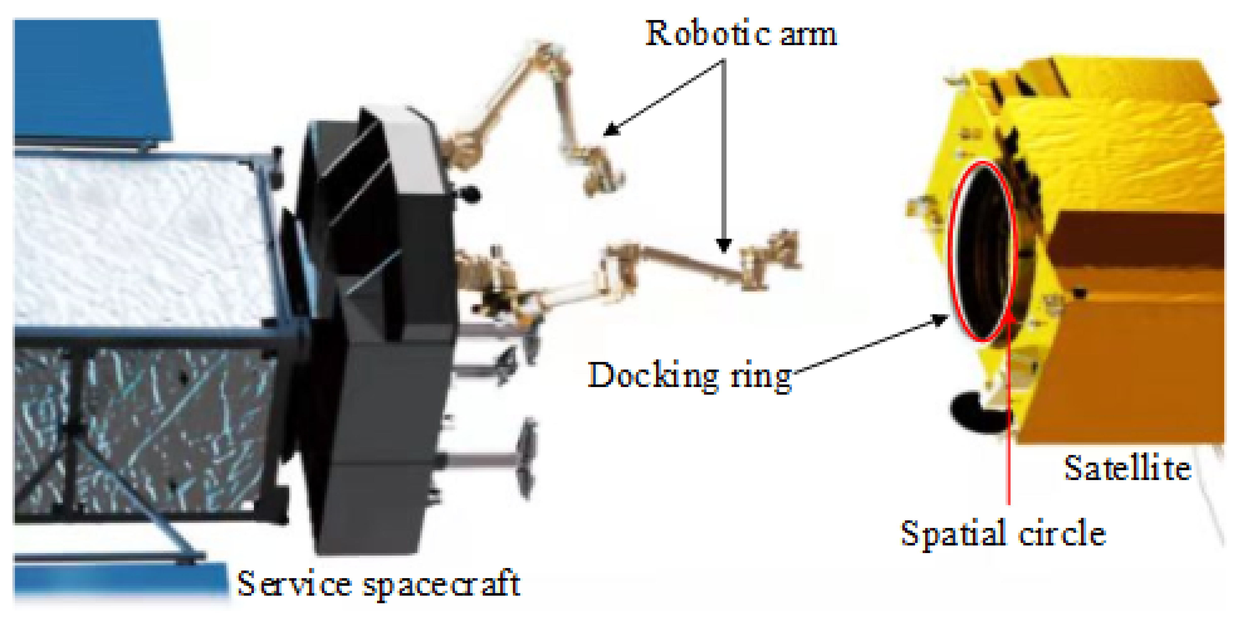
The authors of previous literature [1,2,3,4,5,6,7,8,9,10] studied the use of geometric features, such as solar panels, windsurfing boards, and communication antennas, and proposed a solution method based on point features and straight-line features to solve the issue of the target pose. However, the strength of the above components is not strong enough to be captured by space robots. In the actual space environment, because the target satellite state is unknown, it is difficult to distinguish the position of the extracted point features or linear features on the satellite, and it is difficult to obtain the corresponding relationship. Most satellites have docking ring components that are used to mechanically connect with the rocket during launch. The docking ring assembly can provide a typical circular feature for the pose solution and has a strong gripping rigidity. NASA’s OSAM-1 on-orbit service mission plan captures an on-orbit satellite by grabbing the docking ring for fuel replenishment to extend its lifespan. Additionally, it passed ground verification in 2020 [11]. The deorbit plan proposed by the German OHB company is expected to be launched in 2023 to rescue the Envisat satellite, and the target is also the docking ring [12]. Therefore, using the docking ring target to estimate the relative pose has great practical value. The concept of measuring and grasping the docking ring is shown in the Figure 1.

Figure 1.
The concept of measuring and grasping the docking ring.
Miao and Zhu et al. calculated two solutions of the spatial circle pose based on the projection of the spatial circle on the docking ring on the image. They used the distance from a reference point outside the docking ring plane to the center of the circle, which remained unchanged as a constraint to eliminate false solutions and obtain the pose of the docking ring [13]. Cai and Li et al. proposed a pose solution method based on circular features and straight-line features to solve the roll angle and eliminate the ambiguity of the solution [14]. Liu and Zhao et al. proposed a method for deriving pitch, roll, and yaw angles based on circular features. This method required accurate diameter features to calculate the orientation angle [15]. Liu and Xie et al. proposed a method for estimating circular feature poses based on binocular stereo vision. Although this method did not require other constraints, it had high requirements for the matching results of image features in two different cameras. Thus, the accuracy was easily affected by the matching result [16]. Wang and Zhang proposed an ellipse feature extraction method through texture boundary detection, which provided a new idea for detecting elliptical features on the docking ring, but it still needed to introduce other constraints to solve the pose [17]. Li and Hao et al. proposed a method for solving the position and orientation of the docking ring based on line structured light. By introducing a line structured light device, the relative position and orientation of the docking ring were calculated using the feature of the intersection formed by the actively projected line structured light and the docking ring [18]. To solve the ambiguity of the pose solution caused by the imaging characteristics of the single spatial circle, the above methods required additional external image features, accurate image matching results, or the introduction of other auxiliary measurement devices, in addition to the maintenance of accurate calibration relationships, which are likely to introduce additional measurement errors. Therefore, the above methods have certain limitations in practical applications.
In the actual space environment, the qualitative difference between the image features of the docking ring on the satellite and the background is small, and because the satellite itself is covered with a heat-controlled coating material, the material has a strong reflective effect, and thus, there are more interference features when reflecting light. The lighting conditions in space vary greatly, and the contrast between the target and the background changes with changes in lighting conditions. Second, because the target satellite’s orbital motion state is unknown, it may be three-axis stable or spinning irregularly, which may cause the original docking ring circular feature to be degraded and missing to varying degrees, making it difficult to extract.
In response to the above problems, first, the imaging characteristics of a single spatial circle in the camera model and the reasons for the ambiguity are analyzed. The spatial circle position and orientation are then derived and modeled to recover the pose of the target object from a single RGB image.
This paper proposes a specific discrete point selection method, which discretizes the spatial circle into a set of 3D specific sparse points, eliminates the strict central symmetry of the circle, and then handles the high fusion of the foreground and the background in the image under complex lighting conditions caused by many interference features. Traditional methods have difficulty extracting the 2D sparse points of the feature circle obtained by spatial circle projection. A two-stage pose solving neural network, Hvnet, based on Hough voting, is proposed to extract the features and determine the pose parameters. The first stage of the network learns the direction vector field of each pixel in the docking ring area in the image pointing to the sparse point of the feature circle in the image. The second stage learns the Gaussian heatmap of the sparse point position of the feature circle in the image, and then uses the obtained sparse point direction information and position information to vote pixel-by-pixel to obtain the coordinates of each sparse point of the feature circle. Finally, the spatial circle pose parameters are obtained by the EPnP algorithm [19]. The experimental results show the effectiveness of the method and that it has strong robustness in complex lighting conditions.
2. Definition of Coordinate Frame and Ambiguity Elimination
2.1. Coordinate Frame Definition
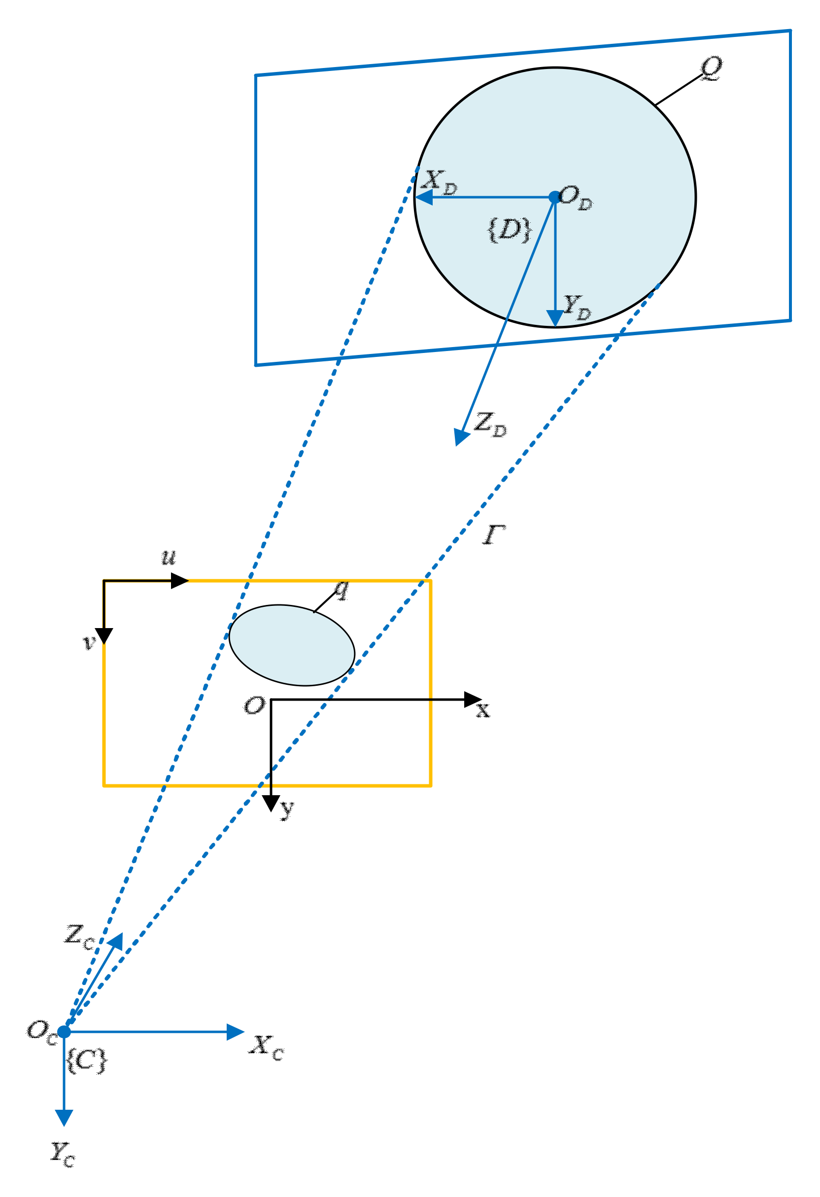
To facilitate the analysis, the camera coordinate frame as shown in the Figure 2 is established. The docking ring plane coordinate frame is defined at the center of the spatial circle. Image coordinate frame and image plane coordinate frame can also be defined. is the camera center point, is the spatial circle with radius on the target of the docking ring, is its center, and is the projection on the image coordinate frame. The position and orientation of the spatial circle are derived in the camera coordinate frame.
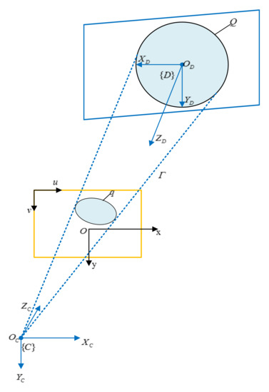
Figure 2.
Coordinate frame definition.
With the exception of extreme cases (the spatial circle is depicted as a straight line), the projection of the spatial circle on the image plane is a circle or an ellipse. When the projection of the spatial circle on the image plane is an ellipse, the optical center of the camera and the spatial circle form an elliptical cone . Additionally, the elliptical cone will also project an image through it. Determining the position and the orientation of the spatial circle is equivalent to finding a cutting plane that cuts the elliptical cone in space Thus, after the plane cuts the elliptical cone, it intersects the elliptical cone to form a circle with a radius of R. Due to the imaging characteristics, the final solution results in two spatial circles with different positions and orientations, one of which is a false solution.
According to the literature [13], the position of the center of the spatial circle and the orientation of the spatial circle in the camera coordinate frame can be obtained as follows:
elliptical cone parameters are the elements of the diagonal matrix of the matrix formed by the parameters of the elliptic general equation. is the orthogonal matrix of the matrix formed by the parameters of the elliptic general equation, . From the above equation, when the spatial circle is depicted as an ellipse, there are two sets of feasible solutions for the position and orientation of the spatial circle, and they are only related to their own projection characteristics. Therefore, when using a single spatial circle to derive poses, the traditional method cannot directly obtain the true solution and needs additional constraints.
In the image coordinate frame, the two spatial circles are depicted as ellipses with the same shape and size. However, when the spatial circle is in the plane of the docking ring, there is only one set of correspondences between the position of the ellipse in the image coordinate frame and the position of the spatial circle in the docking ring plane coordinate frame. The pose relationship of the spatial circle relative to the camera coordinate frame is uniquely determined at this time. Therefore, determining the spatial circle pose restores the target object pose from a single RGB image, and then the true solution can be directly obtained from the image. In recent years, deep learning technology has developed rapidly. For this problem, many current methods have two stages. First, the key points of the target object are detected, and then the EPnP algorithm is used to derive the pose [19]. This two-stage method has achieved the most advanced results [20,21,22,23,24,25]. Inspired by these methods, the spatial circle is first discretized into a set of asymmetric specific sparse points.
2.2. Sparse Point Selection
To avoid ambiguity between discrete points, it is necessary to obtain a set of discrete points that do not have a symmetric relationship. In the polar coordinate system, the following judgments are made. Symmetrical discrete points are equivalent to at least a pair of equal central angles. Therefore, any two central angles that are not equal must be asymmetric. To prove this below, we suppose there are k discrete points.
First, the axis of symmetry is the vertical bisector of two points on the circle, and thus, it must pass through the center of the circle. Then, all k points are connected to the center of the circle, and the central angle is considered. Next, the symmetry proves to be equivalent to the existence of at least a pair of equal central angles.
- (1)
- Symmetry can be obtained if the central angles are equal
In case 1, the two angles have a common edge, as shown in the Figure 3 below. The angle α and the angle β are equal, and points A, B, and C are symmetrical regarding the symmetry axis passing through point B.
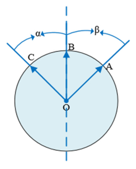
Figure 3.
Two angles have a common edge.
In case 2, the two angles do not have a common edge; as shown in the Figure 4 below, angle α and angle β are equal, and points A, B, C, and D are symmetrical regarding the vertical bisector of BD.
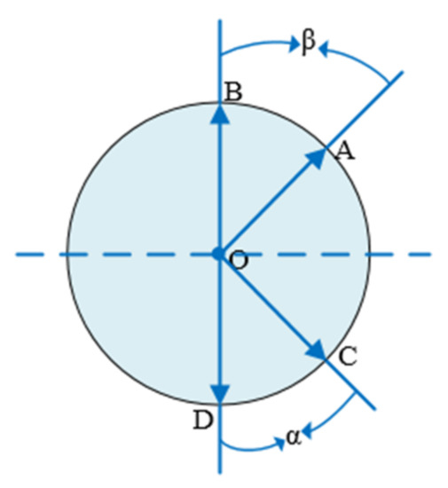
Figure 4.
Two angles do not have a common edge.
- (2)
- At least one pair of equal central angles can be obtained if there is symmetry
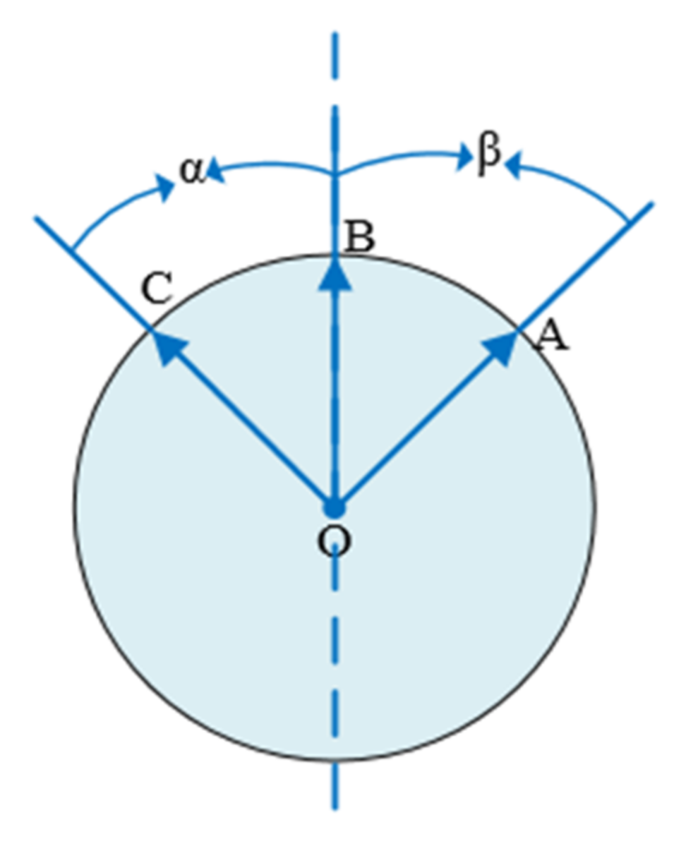
In case 1, the three points are symmetrical. As shown in the Figure 5 below, points A, B, C, and the axis of symmetry must pass through a point. The angles formed by this point and the remaining two points are equal; the angle α and the angle β in the Figure are equal.
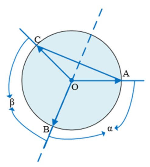
Figure 5.
Three points are symmetrical.
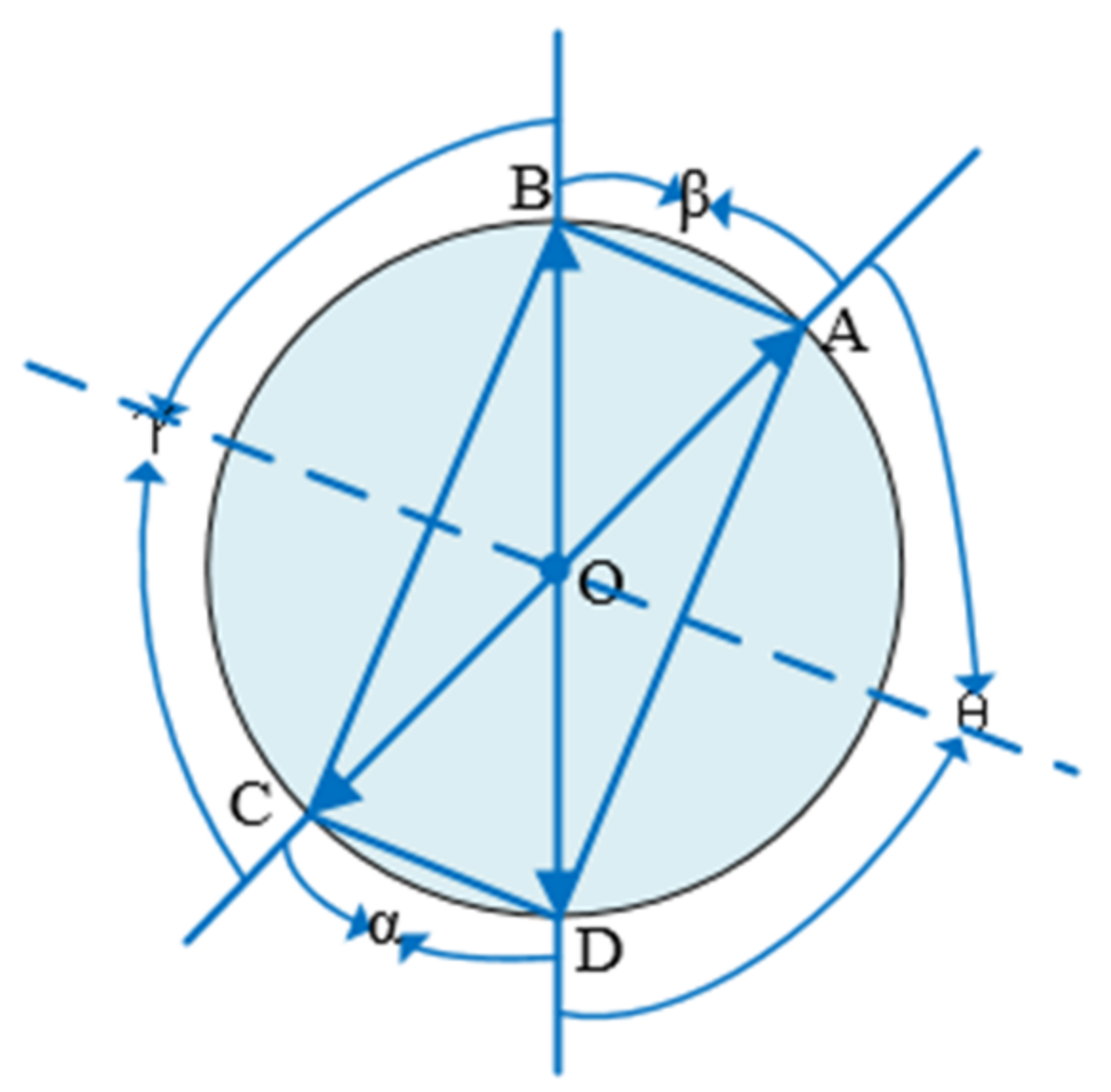
In case 2, the four points are symmetrical, and points A, B, C, and D are shown in the Figure below. There are two situations as follows. In the first case, the axis of symmetry passes through the point itself, as shown in Figure 6. The angle α and the angle β are equal, and the angle θ and the angle γ are equal. In the second case, the axis of symmetry does not pass through the point itself, as shown in Figure 7. The same can be obtained where the angle α and the angle β are equal and the angle θ and the angle γ are equal.
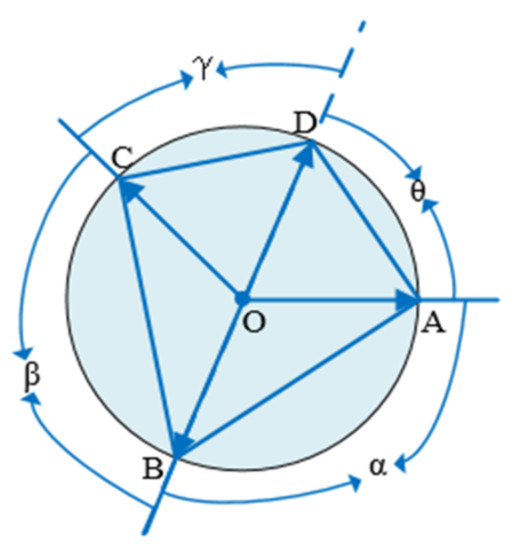
Figure 6.
Four points are symmetrical (case 1).
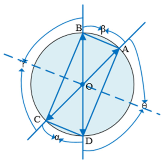
Figure 7.
Four points are symmetrical (case 2).
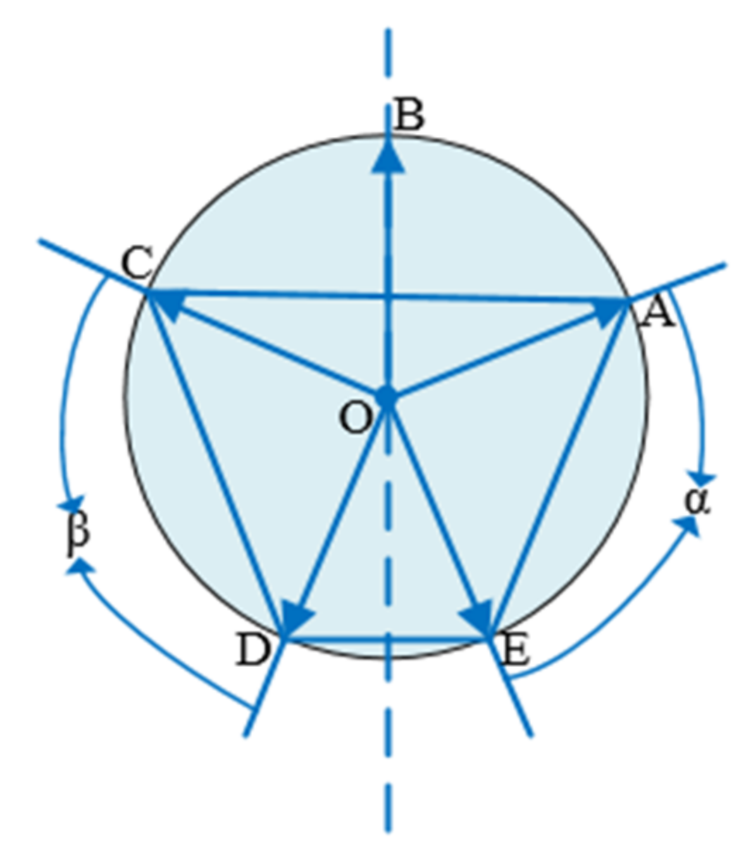
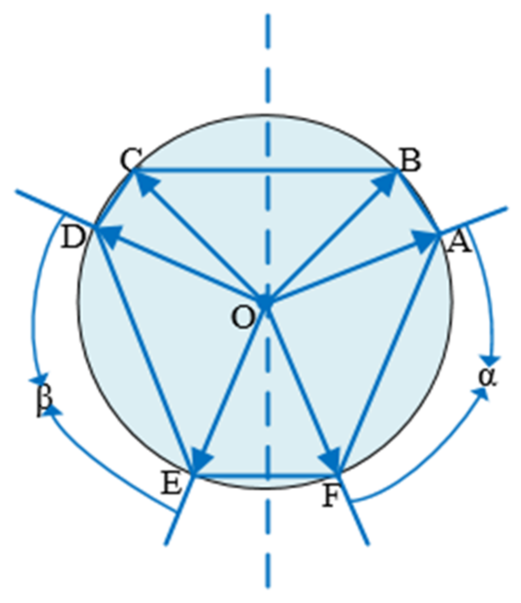
In case 3, if more than five points are symmetrical, there must be more than two symmetric point groups. As shown in Figure 8 below, points A, B, C, D, and E are symmetrical. Points A, C and D, E are symmetrical point groups, and then there are angles α and β, which are equal. As shown in Figure 9 below, points A, B, C, D, E, and F are symmetrical. Points A, D and E, F are symmetrical point groups, and also angles α and β are equal to each other.
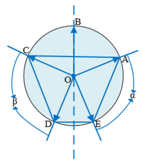
Figure 8.
Five points are symmetrical.
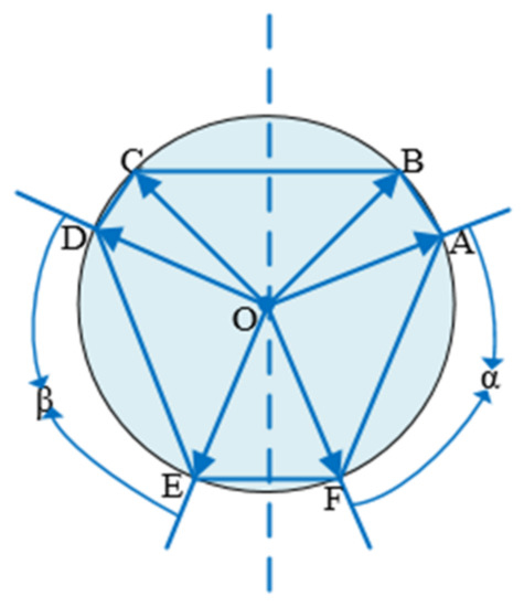
Figure 9.
Six points are symmetrical.
From Case (1) and (2), point symmetry is equivalent to at least a pair of equal central angles. With this equivalence, the definition of symmetry here refers to any point of axis symmetry with more than two points. In addition, to avoid making the sum of two angles equal to the sum of the other two angles, resulting in partial point symmetry, all included angles less than 180° need to be considered. k points have angles, and do not consider angles greater than 180° because, in a circle, there cannot be two angles greater than 180° that will be equal. Thus, there are angles, not only k angles. This is the proof of the k points. Then, the ones that are not equal are selected and are arranged by the angle value.
The angle selection method in this paper shows that in the polar coordinate frame, the initial angle α is set first, in addition to the initial central angle value β. Then α plus β enables us to obtain the next angle. We let β continue to increase, and the increment is obtained from the arithmetic sequence, such as {1:2:3:…:n}. If the increment obtained at a certain time does not meet the condition, the next position of the arithmetic sequence is continued to be used as the increment. Through experiments k = 8, α = 60°, and β = 32°, we can make the sparse points uniformly distributed on the circle and achieve the best performance. Finally, the angle value of the sparse point is {60,92,125,160,198,240,287,342}, and the distribution of the point cloud model in the docking ring is shown in the Figure 10 below.
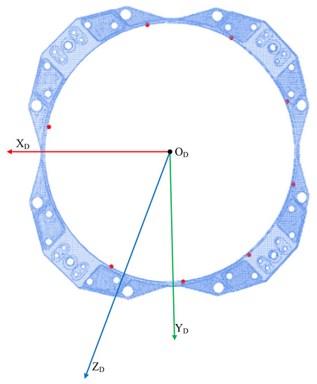
Figure 10.
Sparse point distribution.
3. Pose Estimation Network, Hvnet, Based on Hough Voting
At present, the mainstream methods for locating key points are divided into two types. One type is directly based on the heatmap to return the key point position coordinates; this requires a deep feature extraction network, which has difficulty meeting the requirements of lightweight networks [26,27,28]. The other type of method involves learning the vector field representation of the pixels of the target area pointing to the key points. Thus, the direction of each pixel can be predicted to the key points of the target, and finally, the key point position coordinates are obtained through the intersection point assumption, which can meet the needs of lightweight networks, although the final solution accuracy is not high [29,30,31]. The early work used direct regression to predict key points; however, directly letting the network output two-dimensional coordinates for optimization learning is an extremely nonlinear process, the loss function has weak constraints on weights, and the model has poor generalization ability. The advantage of this method is that the output is the coordinate point, the training and forward speed can be very fast, and it is end-to-end full differential training [32,33].
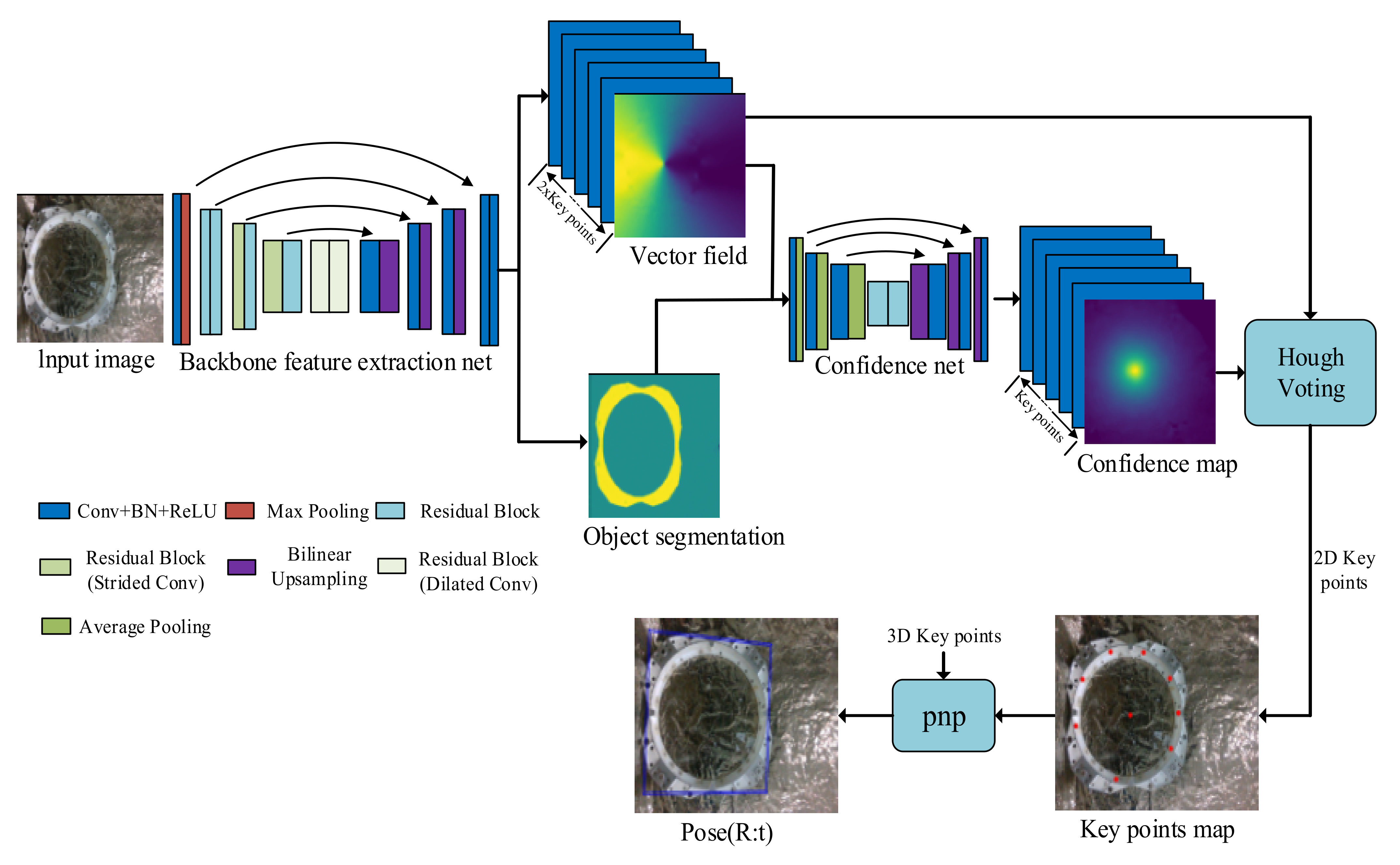
Based on the vector field representation method, the key points are located by the assumption of the intersection point, which is actually a method of using the rigid body characteristics of the object to return to the key point coordinates. Each key point is solved independently, and the mutual positional relationship between the key points is missing. Therefore, the accuracy of the solution is limited, and the method based on the heatmap can not only learn the mutual positional relationship between the key points but can also suppress the response of the non-key points. Aiming at the task of estimating the pose of the docking ring target on the satellite, this paper describes using the method based on the heatmap to improve the previous method based on vector field representation. A lightweight 6D pose solution framework, Hvnet, is also proposed. By inputting an RGB image, we can detect the target in real time and solve its 6D pose at the same time. The 6D pose(R; t) is transformed from the docking ring coordinate frame to the camera coordinate frame. R represents three-dimensional rotation and t represents three-dimensional translation.
The overall framework of the network is shown in the Figure 11 below, which consists of the backbone feature extraction network in the first stage and the heatmap regression network in the second stage. The backbone feature extraction network learns the direction information of the sparse points on the image, and the heatmap regression network learns the probability distribution of the sparse point position. Finally, by the vote method based on Hough voting, the 2D position coordinates of the sparse points of the spatial circle projected into the image coordinate frame are obtained [34]. The method described in this paper uses a pixel-level voting network to detect 2D sparse points in a traversal manner. This method maintains the dense detection of sparse point positioning. It combines the advantages of the two methods and is a dense detection method based on key points that can achieve higher solution accuracy.
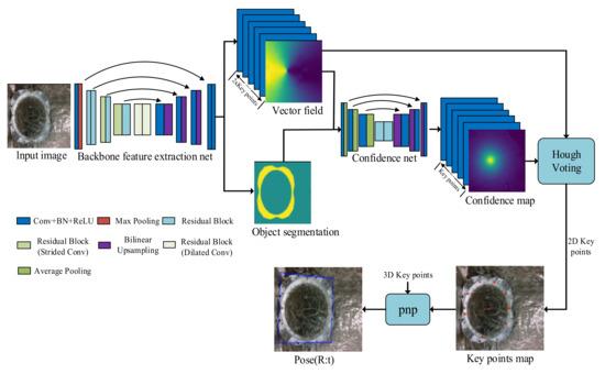
Figure 11.
The network structure Figure.
3.1. Backbone Feature Extraction Network
As shown in the Figure above, the backbone feature extraction network performs two tasks: predicting the semantic segmentation mask and the direction vector field [29]. The input size of the network is , the output size of the vector field is , and the output size of semantic segmentation is . For each pixel of the image, the semantic label belonging to the docking ring target is output and the direction vector pointing to the 2D sparse point is . In this paper, k = 9, including 8 sparse points and the center of the spatial circle, H = 480, W = 640. The direction vector is defined as follows [29]:
Due to the high real-time requirements of the pose estimation task and the memory limitation of the onboard computer, such as the Beckhoff C6015-0010 industrial computer commonly found on commercial satellites, this paper does not use the HRnet high-resolution network, which is currently the most advanced feature extraction network [35]. The backbone feature extraction network uses ResNet18 as the encoding structure. In the encoding stage, a series of convolution and pooling operations are carried out to reduce the feature spatial dimension. When the size of the feature map of the network is equal to , the feature map is no longer processed and downsampled.
In the decoding stage, the target details are gradually restored through three upsampling operations and multiple feature fusions. Additionally, residual blocks are embedded to prevent network overfitting. Skip connection between the main network coding layer and the decoding layer is used to realize the fusion of the deep and shallow features of the network, reducing the loss of positioning information and improving the positioning accuracy.
The loss function of the direction vector is as follows:
The loss function of semantic segmentation is as follows:
3.2. Heatmap Regression Network
In the second stage, a heatmap regression network, confidence net, is introduced. The confidence net network structure is shown in Figure 11 above. It is a symmetric encoder-decoder structure. The input size is H × W × (2 × k + 1) and the output size is H × W × k. Three downsampling operations are performed to make the feature map become the original 1/8(H,W). After two residual blocks, three upsampling operations are performed until the output is H × W, and skip connection is introduced. This structure is more convenient for feature fusion of the same resolution and fusion of more low-level features.
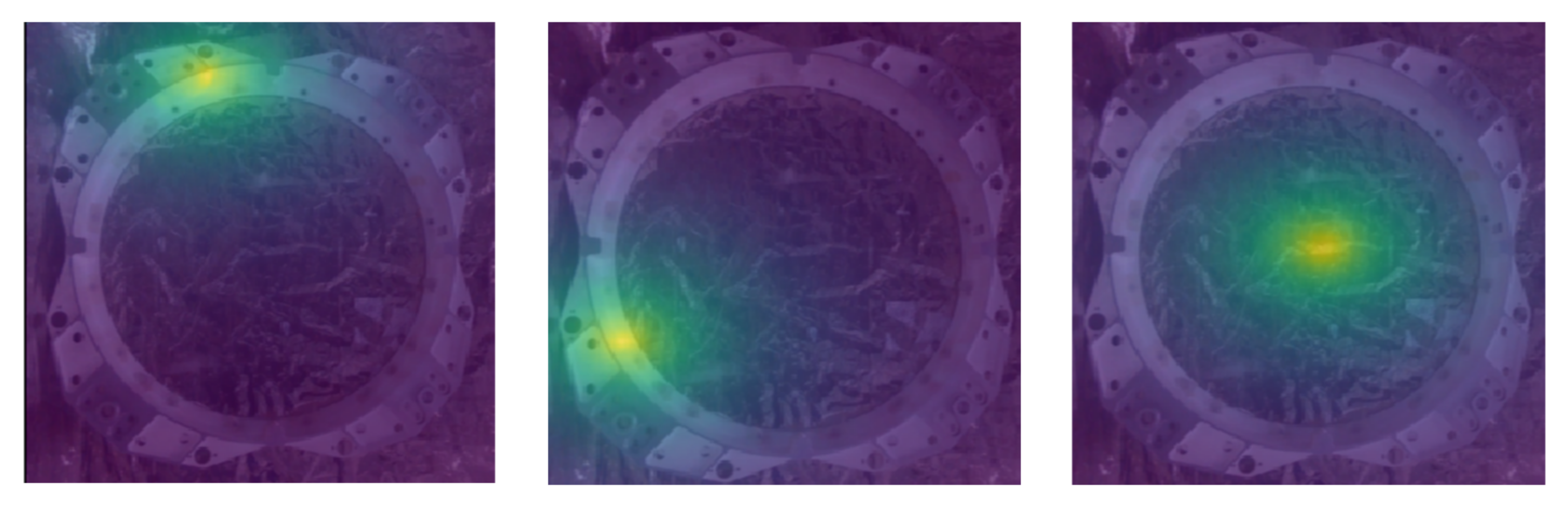
The heatmap label is generated using a Gaussian filter, where the response value of each point represents the probability that the point is a sparse point, and the maximum probability value point represents the sparse point predicted by the network. To facilitate the calculation of the loss, Gaussian filtering is used on the true value to obtain the heatmap [26]:
where k represents the k-th sparse point, represents the probability that the k-th sparse point in the heatmap of the true value is at the position of the pixel point p, the probability of the pixel on the sparse point is 1, and the surrounding pixels spread according to the distance in Gaussian distribution—the farther the distance, the lower the probability; the closer the distance, the higher the probability.
represents the real coordinates of sparse point k, and is the standard deviation of the Gaussian filter, which is a fixed parameter used to adjust the width of the Gaussian function. In this study, we conducted the experiment with = 0.3.
This study used the L2 loss function. The losses of all sparse points are calculated for a certain prediction result. The equation for calculation is as follows:
where represents the probability of sparse point k at position p, is the heatmap generated by the true value, and the value is 0 or 1. If the sparse point is not visible, then , which does not participate in the calculation of the loss. The heatmap generated by the real label value is shown in the Figure 12, which displays the heatmap of three sparse points, and the position of the largest response value in the heatmap corresponds to the position of the sparse point.

Figure 12.
Position response heatmap.
The total loss function of Hvnet is as follows. During training, the Adam optimizer was used to set the initial learning rate to 0.001, which was halved every 20 epochs, and a total of 300 epochs were trained [36].
3.3. Voting Strategy
To obtain the coordinates of the center of the docking ring in the image and the position coordinates of the sparse points in the image, a Hough voting layer was designed and integrated into the network. The voting score of each position in the image is calculated, and the voting score indicates the probability that the corresponding image position is a sparse point. Voting process is shown in the Figure 13 below. Specifically,
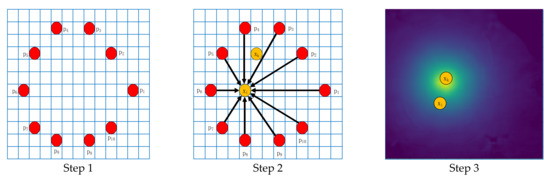
Figure 13.
Voting process.
Step 1: In the image docking ring area, the farthest distributed seed point set is obtained according to the farthest point sampling, , n = 10;
Step 2: For a sparse point , we first calculate the direction vector set of each point of the seed point set pointing to pixel of the docking ring area. Then, we calculate the cosine similarity between the vector set and the predicted direction vector set of the seed point pointing to sparse point as the first part of the voting score. Higher scores indicate alignment with more directions.
Step 3: The voting result of each position in the previous step is weighted by the position probability output by the confidence net, and after each pixel of the docking ring area is processed, the final voting score of all image positions is obtained. Then, we choose the sparse point with the highest score.
The voting score is as follows:
4. Experiment
To verify the effectiveness and feasibility of the proposed method, a pose measurement platform based on the docking ring component was built. The experimental platform mainly includes the docking ring model, spacecraft surface wrapping materials, RGB-D camera, laser tracker, high-power halogen lamp, and electric translation stage, as shown in the Figure 14 below. The docking ring model is a satellite backup part of a certain series, and the model diameter is 469 mm. The camera is Intel’s D435i camera, which is used to collect pictures and generate a pose estimation dataset. The resolution is 1920 × 1280, the size is 90 mm × 25 mm × 25 mm, the effective working range of the depth camera is 0.1 to 10 m, and the camera was accurately calibrated in advance [37]. The movement accuracy of the translation stage is 0.1 mm, and the maximum movement distance is 1000 mm. The wrapping material is covered around the docking ring to simulate the external environment of the satellite where the docking ring target is located. A halogen lamp is used as the light source to simulate the lighting conditions of the docking ring target in the space environment.
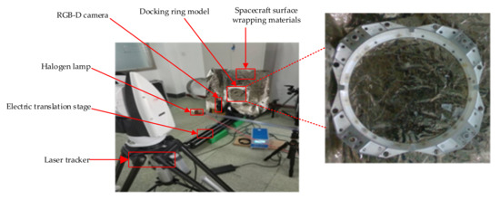
Figure 14.
Pose measurement platform.
The above experimental platform is used to simulate the actual high reflection and many interference space lighting environments of the docking ring target. At different angles and distances, approximately 12,000 images of the docking ring with different poses were collected to generate the docking ring pose estimation dataset. The generation method refers to the LINEMOD dataset [38,39,40]. This dataset was used for training, and some pictures of the dataset are shown in the Figure 15 below.
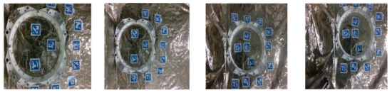
Figure 15.
Part of the image of the dataset.
4.1. Measurement Parameters
Since the docking ring coordinate frame is defined at the center of the spatial circle, the position and orientation of the spatial circle is the relative position and orientation relationship between the docking ring coordinate frame and the camera coordinate frame . The specific equation is expressed as follows:
In general, when the target coordinate frame is the center coordinate frame of the docking ring, since the circle is strictly centrally symmetric, the roll angle cannot be obtained when deriving the pose, but in this study the spatial circle is discretized into a set of 3D asymmetric sparse points. The strict central symmetry of the circle is eliminated. Therefore, when the docking ring model is not an ideal circle model (when rotating at any angle around the z-axis, there is no difference in the image feature), the roll angle can be obtained, and thus, a total of six pose parameters can be obtained. However, when the docking ring model is an ideal circle model, the roll angle cannot be obtained.
For pose(R; t), the physical meaning of the definition is that the coordinate frame of the docking ring first rotates around three coordinate axes, and then the translation coincides with the camera coordinate frame. The rotation sequence is around the X axis, Y axis, and Z axis.
The relative pose involved in this article includes the position amount and orientation angle. The orientation angle is defined as the rotation around X, Y, and Z. The position amount refers to the translation from the origin of the camera coordinate frame to the origin of the docking ring coordinate frame.
4.2. Analysis of the Results
In the experiment, the camera was installed and fixed on the translation stage. The halogen lamp was set to the maximum power of 2000 watts for irradiation, the camera was simulated in a high light intensity, high reflection working environment in space, and then the translation stage was controlled to move the camera forward along the camera coordinate frame , each time moving 10 mm. It moved a total of 40 positions, bringing the camera closer to the docking ring. Because the camera was controlled to move along the Z axis of its coordinate frame, there was no relative rotation, only relative translation. Therefore, the direction of the docking ring relative to the camera remained unchanged, and the direction change should be zero. Finally, the relative movement of the docking ring in the camera coordinate frame was compared with the actual movement of the camera in the translation stage, and the position error and the orientation error of the docking ring could be obtained.
4.2.1. Analysis of the Experimental Results of the Position Error
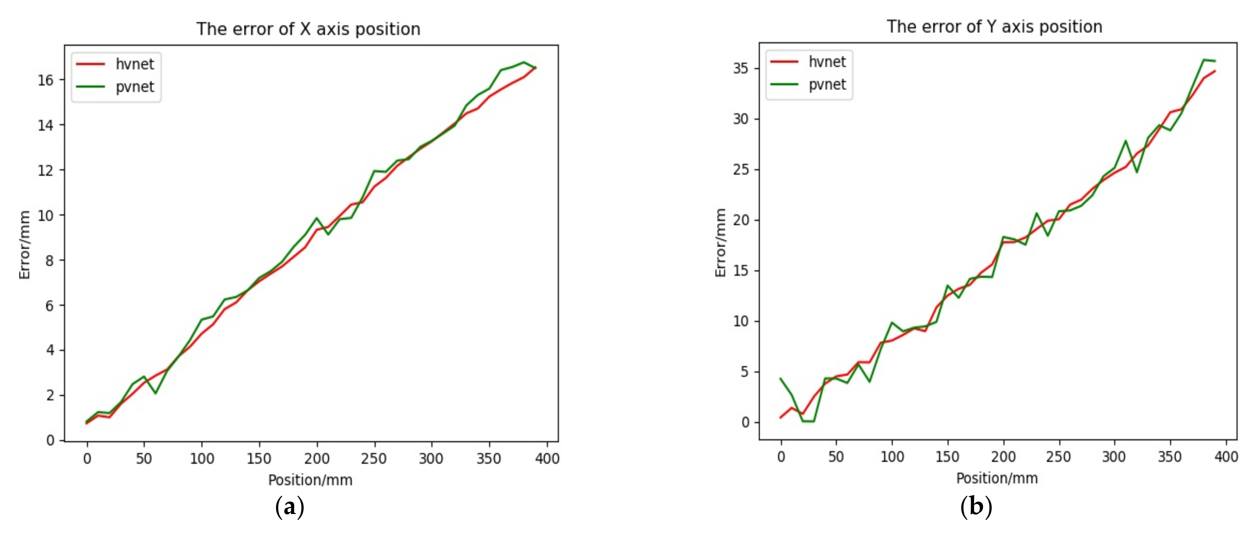
We adopted the method based on the vector field to locate the key points and the Hvnet method proposed in this paper to determine the pose. Considering the practical application scenario of the method in this paper, the network model needs to be lightweight, the memory footprint must be small, and the pose should be estimated in real-time. At present, the use of a single RGB image input can meet the above requirements, and PVNet is the most advanced method. The vector field method uses the most advanced lightweight pose estimation network, PVNet, under the same single RGB image input for comparison [29]. The calculated translation components in pose(R; t) are compared with the relative position components of the camera on the translation stage relative to the initial position, and the position error curve is obtained as shown in the Figure 16 below.


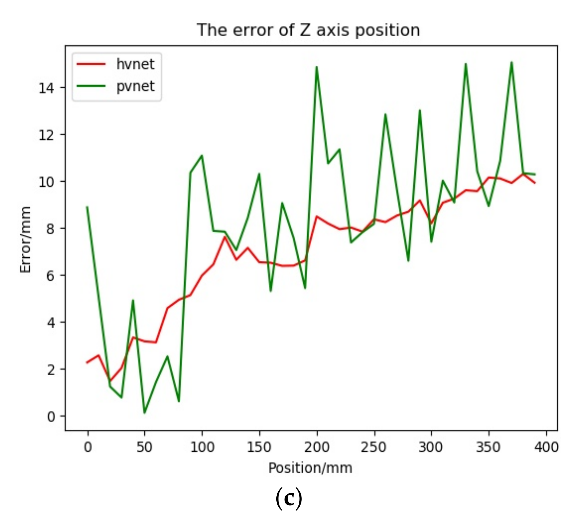
Figure 16.
Position error Figure. (a) Error curve of X-axis direction. (b) Error curve of Y-axis direction. (c) Error curve of Z-axis direction.
The relevant position error experimental data are as follows:
represents the absolute translation error, represents the relative error, is the distance that the translation stage moves relative to the initial position, and is the distance that the docking ring moves relative to the initial position in the camera coordinate frame obtained according to the model.
First, in the X-axis direction, observing the position error curve and Table 1, it can be seen that although the values are relatively close, the results predicted by Hvnet are smoother than those predicted by PVNet. It can also be seen in the Y-axis direction that Hvnet performs better. In the Z-axis direction of the real movement, there is not much difference between the mean value of the absolute translation error and the standard deviation of the absolute translation error, but the maximum absolute translation error of PVNet is 4.8 mm larger than that of Hvnet. The relative error performance is more obvious; the maximum relative error of PVNet is 28% larger than that of Hvnet. Reflecting the error curve, the prediction results of PVNet show obvious fluctuations, whereas Hvnet is relatively stable. From the above, Hvnet is better than PVNet when estimating the position.

Table 1.
Position error data.
4.2.2. Analysis of Experimental Results of the Rotation Angle Error
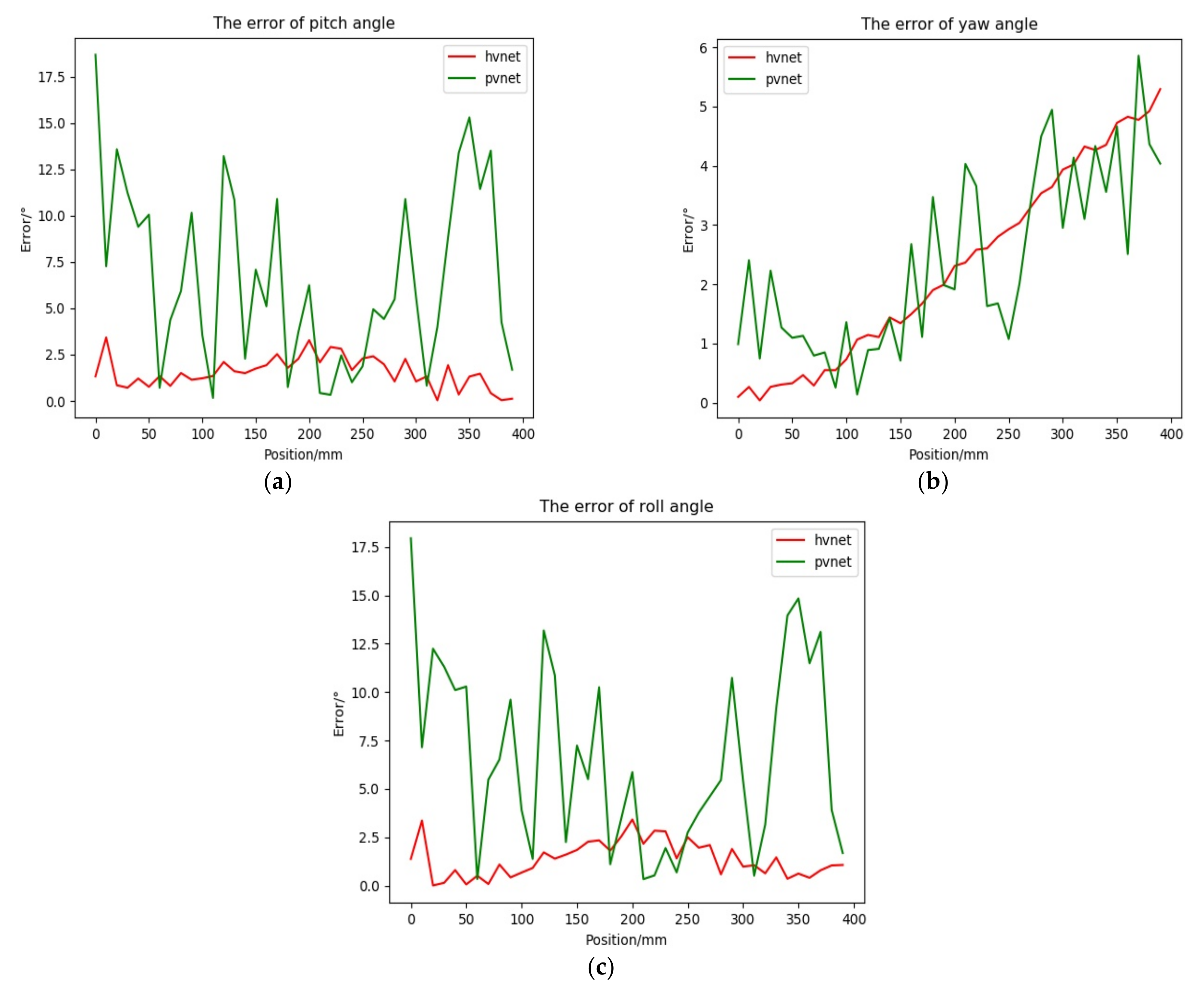
Based on the calculated rotation matrix in pose(R; t), according to Equation (11), the error curves of the rotation angles of the docking ring around the three axes of the camera coordinate frames X, Y, and Z were calculated, as shown in the Figure 17 below.
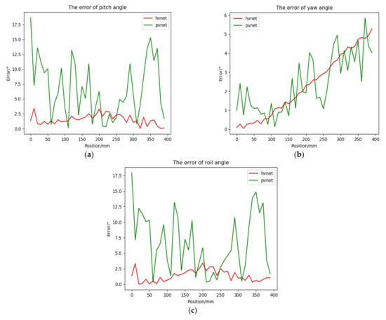
Figure 17.
Rotation angle error Figure. (a) Pitch angle error curve. (b) Yaw angle error curve. (c) Roll angle error curve.
The relevant angle error experimental data are as follows:
represents the absolute value between the corresponding rotation angle of the i-th position and the starting position, and represents the amount of angular error change during the movement.
First, at the pitch angle, observing the error curve and Table 2, it can be seen that the Hvnet solution error variation range is small, the solution accuracy is higher, the maximum angle error is 3.4°, and the average value is 1.5°. The PVNet solution error variation range is larger. The solution accuracy is low, the maximum angle error is 18.6°, and the average value is only 6.6°. In the yaw angle, the difference between the two error values is small, and the maximum error, the mean error, and the standard deviation error are relatively close, but Hvnet is considerably more stable. Regarding the roll angle, Hvnet performs better in terms of solution accuracy and solution stability.
Table 2.
Angle error data.
Similar to the case of estimating the position quantity, Hvnet is also considerably better than PVNet when estimating the angle quantity. Based on the above analysis, using the heatmap regression network to learn the relationship between the key points is very effective for improving the location of the vector field key points result, and the stability and prediction accuracy of the key points prediction is improved under complex lighting environments.
5. Conclusions
Aiming at docking rings that are common in space satellite pose estimation tasks, a pose estimation method based on a single spatial circle is proposed. The spatial circle is first discretized into a set of specific sparse points, and then, when locating 2D sparse points in the image, a two-stage pose estimation network based on Hough voting is proposed to solve the pose parameters. This method does not need to introduce other additional constraints to estimate the pose of the docking ring. Experiments were conducted to verify the effectiveness of the proposed method and achieve good solution accuracy in complex lighting environments. The method proposed in this paper not only realizes the pose solution of the docking ring target but also provides a new idea for estimating the pose of spacecraft, which can provide fixed circular features or symmetrical objects. The improvement in the solution accuracy mainly relates to the neural network model, which enables improving the feature learning ability without significantly increasing the model’s size. In the following step, we will attempt to use spatial and channel attention mechanisms.
Author Contributions
Conceptualization, W.Z. and P.X.; methodology, P.X.; validation, W.Z., P.X. and J.L.; writing—original draft preparation, P.X.; writing—review and editing, W.Z., P.X. and J.L.; project administration, W.Z. and J.L.; funding acquisition, W.Z. and J.L. All authors have read and agreed to the published version of the manuscript.
Funding
The work was supported by the Strategic Priority Research Program on Space Science, the Chinese Academy of Science (Grant No. XDA1502030505), the Foundation of State Key Laboratory of Robotics (Grant No.2019-Z06), and Liao Ning Revitalization Talents Program (Grant No. XLYC1807167).
Institutional Review Board Statement
Not applicable.
Informed Consent Statement
Not applicable.
Data Availability Statement
Data available on request to the author.
Conflicts of Interest
The authors declare no conflict of interest.
References
- Renato, V.; Marco, S.; Palmerini, G.B. Pose and Shape Reconstruction of a Noncooperative Spacecraft Using Camera and Range Measurements. Int. J. Aerosp. Eng. 2017, 2017, 4535316. [Google Scholar]
- Song, J.; Cao, C.; Pennock, G.R. Pose Self-Measurement of Noncooperative Spacecraft Based on Solar Panel Triangle Structure. J. Robot. 2015, 2015, 472461. [Google Scholar] [CrossRef]
- Arantes, G., Jr.; Rocco, E.M.; da Fonseca, I.M.; Theil, S. Far and proximity maneuvers of a constellation of service satellites and autonomous pose estimation of customer satellite using machine vision. Acta Astronaut. 2010, 66, 1493–1505. [Google Scholar] [CrossRef] [Green Version]
- Oumer, N.W.; Panin, G. Tracking and Pose Estimation of Non-Cooperative Satellite for on-Orbit Servicing. In Proceedings of the i-SAIRAS 2012, Turin, Italy, 4–7 September 2012. [Google Scholar]
- Zhang, H.; Jiang, Z.; Elgammal, A. Satellite recognition and pose estimation using homeomorphic manifold analysis. IEEE Trans. Aerosp.Electron. Syst. 2015, 51, 785–792. [Google Scholar] [CrossRef]
- Shu, A.; Pei, H.; Duan, H. Trinocular stereo vision measurement method for spatial non-cooperative targets. Acta Opt. Sin. 2021, 41, 163–171. [Google Scholar]
- Zhang, Y. Research on Visual Measurement Method of Spatial Non-Cooperative Target Based on Straight Line Feature; National University of Defense Technology: Hunan, China, 2016. [Google Scholar]
- Martínez, H.G.; Giorgi, G.; Eissfeller, B. Pose estimation and tracking of non-cooperative rocket bodies using time-of-flight cameras. Acta Astronaut. 2017, 139, 165–175. [Google Scholar] [CrossRef]
- Huang, P.; Chen, L.; Zhang, B.; Meng, Z.; Liu, Z. Autonomous rendezvous and docking with nonfull field of view for tethered space robot. Int. J. Aerosp. Eng. 2017, 2017, 3162349. [Google Scholar] [CrossRef]
- Du, X.; Liang, B.; Xu, W.; Qiu, Y. Pose measurement of large non-cooperative satellite based on collaborative cameras. Acta Astronaut. 2011, 68, 2047–2065. [Google Scholar] [CrossRef]
- Reed, B.B.; Smith, R.C.; Naasz, B.J.; Pellegrino, J.F.; Bacon, C.E. The Restore-L Servicing Mission. In Proceedings of the AIAA SPACE, Long Beach, CA, USA, 13–16 September 2016. [Google Scholar]
- Wieser, M.; Richard, H.; Hausmann, G.; Meyer, J.-C.; Jaekel, S.; Lavagna, M.; Biesbroek, R. E. Deorbit Mission: OHB Debris Removal Concepts. In Proceedings of the ASTRA 2015—13th Symposium on Advanced Space Technologies in Robotics and Automation, Noordwijk, The Netherlands, 11–13 May 2015. [Google Scholar]
- Miao, X.; Zhu, F.; Ding, Q.; Hao, Y.; Wu, Q.; Xia, R. Monocular visual pose measurement method of aircraft based on star-arrow docking ring components. Acta Opt. Sin. 2013, 33, 123–131. [Google Scholar]
- Meng, C.; Li, Z.; Sun, H.; Yuan, D.; Bai, X.; Zhou, F. Satellite pose estimation via single perspective circle and line. IEEE Trans. Aerosp. Electron. Syst. 2018, 54, 3084–3095. [Google Scholar] [CrossRef]
- Liu, L.; Zhao, Z. A new approach for measurement of pitch, roll and yaw angles based on a circular feature. Trans. Inst. Meas. Control 2013, 35, 384–397. [Google Scholar] [CrossRef]
- Liu, Y.; Xie, Z.; Wang, B.; Liu, H. Pose Measurement of a Non-Cooperative Spacecraft Based on Circular Features. In Proceedings of the 2016 IEEE International Conference on Real-time Computing and Robotics (RCAR), Angkor Wat, Cambodia, 6–10 June 2016; pp. 221–226. [Google Scholar]
- Wang, S.; Zhang, S. Spacecraft ellipse feature extraction method based on texture boundary detection. J. Astronaut. 2018, 39, 76–82. [Google Scholar]
- Li, Z.; Hao, Y.; Fu, S. The relative pose measurement method of star-arrow docking ring based on structured light. Comput. Eng. Appl. 2019, 55, 205–212. [Google Scholar]
- Lepetit, V.; Moreno-Noguer, F.; Fua, P. EPnP: An Accurate O(n) Solution to the PnP Problem. Int. J. Comput. Vis. 2009, 81, 155–166. [Google Scholar] [CrossRef] [Green Version]
- Chen, B.; Cao, J.; Parra, A.; Chin, T. Satellite Pose Estimation with Deep Landmark Regression and Nonlinear Pose Refinement. In Proceedings of the IEEE/CVF International Conference on Computer Vision (ICCV), Seoul, Korea, 27 October–3 November 2019. [Google Scholar]
- Sharma, S.; D’Amico, S. Neural Network-Based Pose Estimation for Noncooperative Spacecraft Rendezvous. IEEE Trans. Aerosp. Electron. Syst. 2020, 56, 4638–4658. [Google Scholar] [CrossRef]
- Harvard, A.; Capuano, V.; Shao, E.Y.; Chung, S.J. Spacecraft Pose Estimation from MonocularImages Using Neural Network Based Keypoints and Visibility Maps. In Proceedings of the AIAA Scitech2020 Forum, Orlando, FL, USA, 6–10 January 2020; p. 1874. [Google Scholar]
- Sharma, S.; Ventura, J.; D’Amico, S. Robust model-based monocular pose initialization for noncooperative spacecraft rendezvous. J. Spacecr. Rocket. 2018, 55, 1414–1429. [Google Scholar] [CrossRef] [Green Version]
- Newell, A.; Yang, K.; Deng, J. Stacked Hourglass Networks for Human Pose Estimation. In Proceedings of the European Conference on Computer Vision, Amsterdam, The Netherlands, 11–14 October 2016; Springer: Cham, Switzerland, 2016; pp. 483–499. [Google Scholar]
- Rad, M.; Lepetit, V. Bb8: A Scalable, Accurate, Robust to Partial Occlusion Method for Predicting the 3d Poses of Challenging Objects without Using Depth. In Proceedings of the IEEE International Conference on Computer Vision, Venice, Italy, 22–29 October 2017; pp. 3828–3836. [Google Scholar]
- Cao, Z.; Hidalgo, G.; Simon, T.; Wei, S.-E.; Sheikh, Y. OpenPose: Realtime multi-person 2D pose estimation using Part Affinity Fields. IEEE Trans. Pattern Anal. Mach. Intell. 2019, 43, 172–186. [Google Scholar] [CrossRef] [Green Version]
- Oberweger, M.; Rad, M.; Lepetit, V. Making Deep Heatmaps Robust to Partial Occlusions for 3D Object Pose Estimation. In Proceedings of the European Conference on Computer Vision (ECCV), Munich, Germany, 8–14 September 2018; pp. 119–134. [Google Scholar]
- Papandreou, G.; Zhu, T.; Chen, L.C.; Gidaris, S.; Tompson, J.; Murphy, K. Personlab: Person Pose Estimation and Instance Segmentation with a Bottom-up, Part-Based, Geometric Embedding Model. In Proceedings of the European Conference on Computer Vision (ECCV), Munich, Germany, 8–14 September 2018; pp. 269–286. [Google Scholar]
- Peng, S.; Liu, Y.; Huang, Q.; Zhou, X.; Bao, H. Pvnet: Pixel-Wise Voting Network for 6dof Pose Estimation. In Proceedings of the IEEE/CVF Conference on Computer Vision and Pattern Recognition, Long Beach, CA, USA, 15–20 June 2019; pp. 4561–4570. [Google Scholar]
- He, Y.; Sun, W.; Huang, H.; Liu, J.; Fan, H.; Sun, J. Pvn3d: A Deep Point-Wise 3D Keypoints Voting Network for 6Dof Pose Estimation. In Proceedings of the IEEE/CVF Conference on Computer Vision and Pattern Recognition, Virtual, 14–19 June 2020; pp. 11632–11641. [Google Scholar]
- He, Y.; Huang, H.; Fan, H.; Chen, Q.; Sun, J. FFB6D: A Full Flow Bidirectional Fusion Network for 6D Pose Estimation. In Proceedings of the IEEE/CVF Conference on Computer Vision and Pattern Recognition, Virtual, 19–25 June 2021; pp. 3003–3013. [Google Scholar]
- Toshev, A.; Szegedy, C. Deeppose: Human Pose Estimation via Deep Neural Networks. In Proceedings of the IEEE Conference on Computer Vision and Pattern Recognition, Columbus, OH, USA, 23–28 June 2014; pp. 1653–1660. [Google Scholar]
- Tekin, B.; Sinha, S.N.; Fua, P. Real-Time Seamless Single Shot 6D Object Pose Prediction. In Proceedings of the IEEE Conference on Computer Vision and Pattern Recognition, Salt Lake City, UT, USA, 18–23 June 2018; pp. 292–301. [Google Scholar]
- Xiang, Y.; Schmidt, T.; Narayanan, V.; Fox, D. PoseCNN: A Convolutional Neural Network for 6D Object Pose Estimation in Cluttered Scenes. In Proceedings of the Robotics: Science and Systems (RSS), Pittsburgh, PA, USA, 26–30 June 2018. [Google Scholar]
- Wang, J.; Sun, K.; Cheng, T.; Jiang, B.; Deng, D.; Zhao, Y.; Liu, D.; Mu, Y.; Tan, M.; Wang, X.; et al. Deep High-Resolution Representation Learning for Visual Recognition. IEEE Trans. Pattern Anal. Mach. Intell. 2021, 43, 3349–3364. [Google Scholar] [CrossRef] [Green Version]
- Kingma, D.P.; Ba, J.L. Adam: A Method for Stochastic Optimization. In Proceedings of the International Conference for Learning Representations, San Diego, CA, USA, 7–9 May 2015. [Google Scholar]
- Zhang, Z. A flexible new technique for camera calibration. IEEE Trans. Pattern Anal. Mach. Intell. 2000, 22, 1330–1334. [Google Scholar] [CrossRef] [Green Version]
- Rennie, C.; Shome, R.; Bekris, K.E.; De Souza, A.F. A dataset for improved rgbd-based object detection and pose estimation for warehouse pick-and-place. IEEE Robot. Automat. Lett. 2016, 1, 1179–1185. [Google Scholar] [CrossRef] [Green Version]
- Hinterstoisser, S.; Lepetit, V.; Ilic, S.; Holzer, S.; Bradski, G.; Konolige, K.; Navab, N. Model Based Training, Detection and Pose Estimation of Texture-Less 3d Objects in Heavily Cluttered Scenes. In Proceedings of the ACCV, Deajeon, Korea, 5–9 November 2012. [Google Scholar]
- Garrido-Jurado, S.; Muñoz-Salinas, R.; Madrid-Cuevas, F.J.; Marín-Jiménez, M.J. Automatic generation and detection of highly reliable fiducial markers under occlusion. Pattern Recognit. 2014, 47, 2280–2292. [Google Scholar] [CrossRef]


Publisher’s Note: MDPI stays neutral with regard to jurisdictional claims in published maps and institutional affiliations. |
© 2022 by the authors. Licensee MDPI, Basel, Switzerland. This article is an open access article distributed under the terms and conditions of the Creative Commons Attribution (CC BY) license (https://creativecommons.org/licenses/by/4.0/).