Article

Exploiting Distance-Based Structures in Data Using an Explainable AI for Stock Picking

Faculty of Mathematics and Computer Science, Philipps University of Marburg, Hans-Meerwein Str., 35032 Marburg, Germany
Information 2022, 13(2), 51; https://doi.org/10.3390/info13020051
Submission received: 26 November 2021 / Revised: 2 January 2022 / Accepted: 16 January 2022 / Published: 21 January 2022
(This article belongs to the Special Issue Foundations and Challenges of Interpretable ML)

Abstract

:
In principle, the fundamental data of companies may be used to select stocks with a high probability of either increasing or decreasing price. Many of the commonly known rules or used explanations for such a stock-picking process are too vague to be applied in concrete cases, and at the same time, it is challenging to analyze high-dimensional data with a low number of cases in order to derive data-driven and usable explanations. This work proposes an explainable AI (XAI) approach on the quarterly available fundamental data of companies traded on the German stock market. In the XAI, distance-based structures in data (DSD) that guide decision tree induction are identified. The leaves of the appropriately selected decision tree contain subsets of stocks and provide viable explanations that can be rated by a human. The prediction of the future price trends of specific stocks is made possible using the explanations and a rating. In each quarter, stock picking by DSD-XAI is based on understanding the explanations and has a higher success rate than arbitrary stock picking, a hybrid AI system, and a recent unsupervised decision tree called eUD3.5.

1. Introduction

In stock picking, targeted investment in individually listed companies is made by selecting shares according to certain criteria to achieve an above-average return. However, identifying the appropriate criteria is demanding mainly to two reasons. First, commonly known explanations for such a stock-picking process are too vague to be applied in concrete cases. Second, it is challenging to analyze high-dimensional data with a low number of cases in order to derive data-driven explanations. In principle, decision trees offer themselves as a solution for both challenges by deriving algorithmically specific criteria for stock picking from fundamental data to achieve an above-average return.
In the classical supervised top-down induction of decision trees (e.g., [1,2]), the distance metric or splitting criterion takes into account the class information of each case of data, whereas for unsupervised decision trees, the cases are not classified, and the splitting criterion does not take into account any class information [3]. However, this work focuses on unsupervised approaches because the data described below does not have a classification. In the supervised case, an extensive state-of-the-art survey of explainable methods can be found in [4], whereas in the unsupervised case approaches are less common. In this second case, explainable Ais (XAIs) based on unsupervised decision trees could be useful to derive stock-picking criteria by providing relevant and meaningful explanations based on fundamental data. However, current unsupervised decision trees are restricted by their choice of splitting criterion based on specific cluster assumptions (e.g., spherical cluster structures for the methods of Dasgupta et al. or Loyola-González et al. [5,6]).
This paper’s contribution is the proposition of an unsupervised explainable AI (XAI) based on a decision tree guided by distance-based structures in data (DSD) for non-sequential data. DSD are detected in an unsupervised approach by selecting a distance metric based on multimodality [7] combined with projection-based clustering [8]. The identified DSD guides a supervised decision tree into generating meaningful and relevant explanations evaluated by Grice’s maxims [9,10]. Additionally, this works’ methodology is better reproducible than many other approaches introduced in Section 2 because it is restricted to accessible open-source libraries of CRAN (see Section 3.4 for details).
Stocks are picked by selecting companies of the best-rated leaf of a decision tree. The results are compared to the sophisticated explainable AI proposed by Loyola-González et al. [6] and a rule-based system combined with a neural network, called hybrid AI, of Tsaih et al. [11]) with priorly reported performance due to the low availability of unsupervised explainable AI systems with accessible source code.
The fundamental data of specific companies is analyzed: their shares are tradable in the stock market, and the companies are listed in the German Prime Standard [12]. The Prime Standard is a segment of the regulated market in the Frankfurt stock exchange with additional admission follow-up duties and the highest transparency requirements [13]. Here, stocks of the German Prime standard [13] are selected because companies with tradable shares within this standard [12] must publish their quarterly financial statement, income sheet, and cash flow every three months due to regulations [13]. Results are provided based on four datasets of four consecutive quarters. The results identify, in each quarter, valid DSD that allow for extrapolation about the future behavior of the shares’ market value for a chosen leaf containing a subset of stocks. All four quarters show that the DSD-XAI outperforms a hybrid AI system and a recently published unsupervised decision tree called eUD3.5 [6] for the case of stock picking.

2. Related Works

A considerable number of studies have inferred that predicting stock market returns is a difficult task [14]. Nazario et al. distinguished two main analysis categories that are used for this goal [14], called technical and fundamental analysis. Technical analysis is a set of tools that predict future returns in financial assets by studying past market data such as stock price and volume [14]. For example, the direction of movement of two stock prices indices and two stock prices was predicted with several models of which random forests exhibited the highest performance with around 84% accuracy based on ten technical indicators such as open, high, low, and close prices [15]. Additionally, predicting future values of the same two indices using ten technical indicators was possible up to 30 days in advance with a mean absolute error of around 238 to 927 depending on the model and selected index [16].
However, this work focuses on fundamental analysis. Fundamental analysis determines the expected stock prices by examining financial factors that are meaningful and relevant to the domain expert who searches for stocks that are currently trading at prices that are higher or lower than their actual value. Consequently, “fundamental analysis utilizes economic factors to estimate the intrinsic values of securities, whereas technical analysis relies on historical data on stock prices” [14].
We refer to a company’s accounting information in a given quarter if the company’s shares are tradable in the Frankfurt stock exchange [13]. The implicit assumption of a trade is the goal to increase the investment of the person purchasing or selling the stock shares. This increase is measured by the transaction yield, which will be defined as the rate of return in the methods section. Using specific financial products instead of shares, it becomes unimportant if the return rate is positive or negative as long as this and the correct share of stock are known before the transaction. Often, a fundamental analysis is a part of a more extensive system to select the right stock (e.g., CANSLIM system [17]) using a low amount of variables and a larger number of stocks [18,19,20]. Thus, “research does not fully exploit the wealth of information contained in general purpose financial reports but is outside of the primary financial statements” [21].
As an alternative to the usage of fundamental data, Gite et al. recently proposed to predict stock prices using text mining based on sentiment analysis [22]. They were able to predict the open price of the Indian stock market for seven days with a low error [22] by combining a bi-classification of headlines into positive and negative news with Yahoo’s finance stock price data within an LSTM and the post-hoc explainer called LIME [23].
More generally, there are two approaches to provide explanations from models that could be applied in fundamental analysis. The first approach combines sub-symbolic systems (c.f. [24]) with post-hoc interpretation and justification (e.g., [25]). The second approach comprises of symbolic systems (c.f. [26]) that can be explained through reasoning [27]. Hence, the second type is often called an explainable AI system (XAI) [28] because such systems should be intrinsically explainable [29]. Typical XAIs comprise combinations of neural networks with rule-based expert systems [30,31], Bayesian networks with rule mining [32], hybrids of clustering and fuzzy classification [33] or neuro-fuzzy classification [34], interpretable decision sets [35], or decision tables [36], specific genetic algorithms [37], decision tree clustering [3,38], or clustering combined with generative models [39]. However, most often, no open-source code is provided. An extensive state-of-the-art survey of explainable supervised methods can be found in [4].
However, the focus lies here on unsupervised approaches because the datasets used do not have a classification (see Supplementary Material for details). Most recently, the eUD3.5 decision tree algorithm was proposed by Loyola-González et al. [6] with an accessible implementation. Contrary to supervised decision trees that incorporate the given classification in the split criterion, the eUD3.5 uses an unsupervised split evaluation criterion for which the authors claim that for evaluating the split of features, both separation and compactness are taken into account [6]. The resulting decision tree does not require a parameter to control the depth of the tree. Similar to random forests, Loyola-González et al. [6] propose to build 100 different trees “by selecting the best feature to split from a random subset of features”. For each obtained tree, the authors consider its leaves as partitions of data that can be combined to obtain the number of clusters specified by the user. Please see Section 3.4 for access to implementation.
Another recent approach of Dasgupta et al. [5] used a hybrid of k-means with a decision tree called iterative mistake minimization algorithm (IMM). The k-means method provides the labels and cluster centers with which the decision tree is built top-down using binary splits in which each node of the tree is associated with a portion of the input data [5]. However, Dasgupta et al. [5] did not provide any source code in their work.

3. Materials and Methods

In the sense of the explication provided in Section 2, fundamental analysis is performed in this work. The method chapter is divided into four sections: identification of DSD by cluster analysis and its validation, fundamental analysis, as well as evaluation by Grice’s maxims. Implementation details and access to open-source code is described in Section 3.4.
Contrary to the usual approach, DSD are identified using all features through projection-based clustering, which is able to identify a large variety of DSD [8]. The details are described in Section 3.1. The clustering guides the supervised decision tree of a subset of features selected by domain knowledge of the fundamental analysis. The reasons for the selection can be found in Section 3.2. The choice of method for the supervised tree is motivated in Section 3.3 out of the available trees listed in Section 3.4. Next, explanations are deduced from the decision tree by following each path from the root to leaf. Finally, the explanations are rated and lead to the decision if the price of shares of a group of companies will probably fall or rise. The details are defined in Section 3.3.1. The performance evaluation is based on the expected rate of return for a stock picking in the next respective quarter. The details are described in Section 3.3.2.

3.1. Identification of DSD

Applying web scraping to the Yahoo finance website yields the features describing financial statement, income sheet, and cash flow per company and quarter in the year 2018. Datasets and their features are listed in Supplementary Material. Web scraping resulted in the accounting information of 269 companies’ accounting information in the first quarter and 251 companies’ accounting information in the second quarter, 261 companies’ accounting information for the third quarter, and 286’ companies accounting information for the fourth quarter of 2018. However, fundamental data is not provided with a classification that makes typical supervised XAIs infeasible. The adjusted closing price of a share per day for each company was extracted for the second (3 April 2018 until 29 June 2018) and third quarter (3 July 2018 until 28 September 2018), fourth quarter (1 October 2018 until 31 December 2018), and first quarter (2 January 2019 until 29 March 2019). Companies with accessible stock prices were mapped to their fundamental data. The quarter of fundamental data lies prior in time to the quarter of stock prices. The details are described in Supplementary Table S1. Days were ignored when the stock market was not open (holidays, weekends, etc.). For data access please see Section 3.4. Data analysis was performed for each quarter separately. After preprocessing (i.e., handling of missing values, standardization, and decorrelation) of data, a specific distance metric was chosen based on its property of multimodality [7] investigated by mirrored-density plots [40] and verified by the dip test [41]. The selected multimodal distance matrix is defined by the chord distance in Equation (1) [42]:
D ( x , y ) = 2 ( 1 x y x x y y )
which represents the dissimilarity between the accounting information of each two companies x and y of the high-dimensional feature space. Implementation is accessible as described in Section 3.4.
Then, projection-based clustering [8] guided by a swarm projection method is applied, since swarm intelligence makes the usage of a global objective function unnecessary and allows the usage of specific distance metrics [43]. In the company’s accounting information data, there are no concepts of how a cluster should be defined. Thus, approaches such as PSO [44] or conventional projection or clustering algorithms are unfeasible because global clustering criterions predefined the DSD they seek [45,46]. If a global clustering criterion is given, it follows that an implicit definition of a cluster exists, and the bias is the difference between this definition and the existing structures in data [47]. For example, Single linkage (SL) tends to produce connected and chain-like structures by searching for nearest neighbors in contrast to Ward, which is sensitive to outliers and tends to find compact clusters of equal size with ellipsoidal structures [43].
The projection guides the subsequent hierarchical clustering using the shortest paths of the weighted Delaunay graph of the projection for which the weights correspond to the high-dimensional distance metric chosen [8]. In the dendrogram, substantial changes in fusion-levels of the ultrametric portion of the distance (c.f. [48]) would (y-axis) indicate the best cut. If only slight changes in the fusion levels exist, it indicates that the algorithm is not able to find a cluster structure. Details about the algorithm are described in [8] and are accessible as described in Section 3.4.

Validation of DSD

The cluster tendency is evaluated with a combination of statistical testing [49,50] and a visualization of the mirrored-density plot [40]. Data has an appropriate cluster tendency if the first principal component is multimodal [49,50,51]. Statistical testing for multimodality is performed with the dip test [41]. DSD are valid if the clustering is consistent with the topographic map of high-dimensional structures. The topographic map with hypsometric tints can be visualized after the projection of the high-dimensional data into a toroidal and two-dimensional plane. The topographic map is the visualization for the generalized U-Matrix [52], which means that the altitudes correspond to the dissimilarities (high altitudes represent high dissimilarities and vice versa). Hypsometric tints are surface colors representing elevation ranges (see [53]). Contour lines are combined with a specific color scale. The color scale is chosen to display various valleys, ridges, and basins: blue colors indicate small distances (sea level); green and brown colors indicate middle distances (low hills); and shades of white colors indicate vast distances (high mountains covered with snow and ice) [53]. Superordinate structures in data are visible through valleys and basins, representing clusters and the watersheds of hills and mountains that represent the borders between clusters. In this 3D landscape, the borders of the visualization are cyclically connected with a periodicity (L, C). This visualization is necessary because the Johnson–Lindenstrauss lemma [54,55] states that the scatter plot’s two-dimensional similarities cannot coercively represent high-dimensional distances. In sum, the topographic map can visualize high-dimensional, distance-based structures of a given data set or distance matrix derived from the data set if a dataset possesses cluster structures [45]. A central problem in clustering is the correct estimation of the number of clusters. The topographic map can address this problem since it allows assessing the number of clusters [53] by counting the number of valleys. The points in the topographic map symbolize the companies. After the clustering task is performed, the labels of the clustering color these points. In this sense, the clustering is valid if mountains do not partition clusters indicated by colored points of the same color [45]. Additionally, a heatmap is provided in which the clustering orders the distances with blue to yellow colors indicating low distances and orange to red colors indicating high distances. If the coloring of the map’s ordered pixels indicates that the intracluster distances are smaller than the intercluster distances, then the clustering is valid in the meaning described above.

3.2. Fundamental Analysis

From the available features described in the section before (Section 3.1 and Supplementary Material), the supervised decision tree is restricted to four features, because domain knowledge states for these four features that they are interrelated with the price development of stocks. These four selected features can be easily understood based on information extracted from the web (www.investopedia.com, accessed on 18 September 2018). High values in these features should be interrelated with rising stock prices and low values with falling stock prices. The features are net income from continuing ops, operating income or loss, cash and cash equivalents, and income before tax. The domain knowledge about these features is cited below:
Net income from continuing ops’ defines the after-tax earnings that business has generated from its operational activities, meaning how much a company has in revenue after expenses are deducted. Net income from continuing ops “is considered to be a prime indicator of the financial health of a firm’s core activities”.
‘Operating income or loss’ is the difference between the gross revenues and costs generated by ordinary operations (e.g., cost of goods sold, wages, and depreciation) and before deducting interest, taxes, et cetera. Operating income measures the profitability of a company telling investors how much revenue will eventually become profit. “Earnings before interest and taxes (EBIT) and is also referred to as the operating profit or recurring profit. The one big difference between operating income and EBIT is that EBIT includes any non-operating income the company generates” [56].
“’Cash and cash equivalents’ refer to the line item on the balance sheet that reports the value of a company’s assets that are cash or can be converted into cash immediately,” meaning that they are short-term investments. They are the most liquid assets a company possesses and are one of a company’s crucial health indicators.
“‘Income Before Tax’ combines all of the company’s profits before tax, including operating, non-operating, continuing operations and non-continuing operations.” “ [It] holds much value in providing internal management and external users of financial data with a company’s operating performance”. ‘Income Before Tax’ “emphasizes the general operations of a business”. This makes companies in different states or countries more comparable, as tax rates may differ significantly across borders [56].
In sum, the understanding of selected features allows the explanation of stock prices’ future behavior.

3.3. Searching for Meaningful Explanations Using the Grice’s Maxims

In our work, explainability is evaluated based on the four Grice maxims of relevance, quality, manner, and quantity [9]. For the maxim of relevance, explanations are typically relevant if they are tendentially contrastive (c.f. [57]), which will be used to evaluate the relevance of explanations. The other three maxims are used to select the best-performing decision tree in terms of meaningful explanations, because decision trees may not always be intrinsically interpretable [29]. The maxim of quality states that only well-supported facts and no false descriptions should be reported. Quality will be measured by the accuracy of supervised decision trees guided by the clustering. Accuracy is computed as 1-error. The error is the sum of the number of missing and incorrect classified points divided by their number. The maxim of manner suggest being brief and orderly and avoiding obscurity and ambiguity [9]. Therefore, the decision tree uses only preselected and non-transformed features that can be easily understood based on information extracted from the web (see Section 3.2). The maxim of quantity states that neither too much nor too few explanations should be presented [9] given the limited capacity of human cognition [29]. This work specifies the statement in the sense that the number of explanations should follow the Miller optimum of 4–7 [58,59]. As decision tree algorithms do not aim at meaningful explanations [60], a path from the root to each leaf in this tree corresponds to an explanation. Each explanation based on a path gives precise thresholds of the features depicted in the nodes. Thresholds between low and high are interrelated with rising and falling stock prices. Decisions trees are evaluated according to the criteria quality, quantity, and manner. Then, explanations are meaningful to a domain expert (c.f. discussion [61]).

3.3.1. Rating of Explanations

The explanations are rated as follows. Each path in the tree will have several nodes, with each one having a specific threshold for a particular feature (see Section 3.2), dividing the feature into values lower than the threshold and higher than the threshold. For each node, the score increases by one point if the path follows the higher values and decreases with one point if it follows these features’ lower values. A positive scoring is an indication of rising prices, and a negative scoring indicates falling prices. It follows that positive scores define a long (+), and negative scores a short (−), position. If no tree with sufficient accuracy (>90%) can be found, the scoring is zero. The path having the highest absolute score values is selected, and the explanation describing this path is used for stock picking.

3.3.2. Validation by Evaluation of the Relevance of Explanations

The relevance of the explanation is evaluated based on stock picking as follows. The stock picking is investigated by comparing the rate of the return of shares during each quarter between a cluster and all stocks (defined from here on as the random choice). The rate of return is computed in Equation (2) by the relative difference:
R ( P 1 , P 2 ) = 2 P 2 P 1 P 1 + P 2                            
If P 1 is the adjusted closing price of a share on the first day and P 2 the adjusted closing price of the second day [62], the rate of return of the quarter is defined as the sum over all days in a quarter. It should be noted that it was shown that this definition of the rate of return should be preferred over the log-ratio [62]. The hypothesis that prices in a cluster will rise or fall can be tested under the assumption that all companies’ accounting information data is available on the same date at the beginning of the respective quarter of a year (i.e., no look-ahead bias). Backtesting is conducted with the meaning that all data was available at the start of the analysis. The validation of provided explanations by the DSD-XAI is performed by simulating buying at the beginning of the respective quarter and selling at the end of the quarter with three options: either randomly, by stock picking based on the explanation of the best-rated leaf of the DSD-XAI, or by using eUD3.5. Then, the rate of return per cluster is compared to each other by class-wise box plots. Class-wise boxplots visualize the difference between the random choice and the stock-picking if the dip test is performed prior to plotting to test against multimodality [41]. Additionally, statistical testing with an unpaired two-sided t-test [63] is performed to determine if the means of the random choice versus the stock-picking are significantly different from each other.

3.4. Access to Data and Open-Source Code

All computations were performed in R using an iMac PRO, 32 Cores, 256 GB RAM. All libraries used are accessible via CRAN and published. Furthermore, all dependencies of the libraries used are managed via CRAN. The supervised decisions trees investigated are conditional inference trees (https://cran.r-project.org/package=partykit, accessed on 6 October 2020), CART (https://cran.r-project.org/package=rpart, accessed on 6 October 2020), C45 (https://cran.r-project.org/package=RWeka, accessed on 6 October 2020), C50 (https://cran.r-project.org/package=C50, accessed on 6 October 2020), and the evolutionary learning of globally optimal trees (https://cran.r-project.org/package=evree, accessed on 6 October 2020). In this work, we used for eUD3.5 the C# Code usable through GitHub (https://github.com/miguelmedinaperez/eUD3.5, accessed on 6 October 2020) with the preset of three clusters hardcoded in the source code.
Distance metrics investigated and the one selected can be found in https://cran.r-project.org/package= parallelDist (accessed on 6 October 2020); the dip test for multimodality is accessible via https://cran.r-project.org/package=diptest (accessed on 6 October 2020) and the mirrored-density plot via https://cran.r-project.org/package=DataVisualizations. Other statistical testing and correlation measures used are found in R base. Projection-based clustering, the accuracy implementation, and the evaluation of cluster tendency are accessible in https://cran.r-project.org/package=FCPS, accessed on 6 October 2020 [64]. If not stated in the manuscript specifically otherwise, all algorithms are used in the default parameter setting.

4. Results

The results are divided into three parts: the evaluation of the meaningfulness of explanations, the relevance of explanations, and the identification of DSD by cluster analysis with its validation.

4.1. Meaningfulness of DSD-XAI Explanations

A supervised decision tree guided by DSD for each quarter is computed and exemplarily shown in Figure 1 for the fourth quarter (see Figure 2, Figure 3 and Figure 4 for other quarters). The accuracy of each best-performing decision tree based on the DSD was 93%, 96%, 96%, and 91% for each respective quarter.
The features are presented in the nodes, and the thresholds are written in the edges after the respective node. The explanations extracted from the decision tree of each quarter Q with the highest rating are concise: Q1: NetIncomeFromContinuingOps < 1865 & OperatingIncomeorLoss < 17 , Q2: NetIncomeFromContinuingOps 362 & CashAndCashEquivalents > 932 , 200 , Q3: IncomeBeforeTax < 51 & NetIncomeFromContinuingOps < 313 , 000 , and Q4: CashAndCashEquivalents < 109 , 055 & OperatingIncomeorLoss < 3000 . With these explanations, the hypotheses are as follows: a short position of 59 stocks in quarter two, a long position of 36 stocks in quarter three, a short position of 56 stocks in quarter four, and a short position of 17 stocks in the first quarter of the next year. In sum, the explanations of DSD-XAI are meaningful. The eUD3.5 algorithm provided one big cluster, one small cluster, and one tiny cluster for every quarter. The four quarters yielded 461 (135), 474 (93), 444 (87), and 401 (89) explanations (in form of pattern descriptions) for all clusters (for the small cluster), which are not concise and, hence, not meaningful.

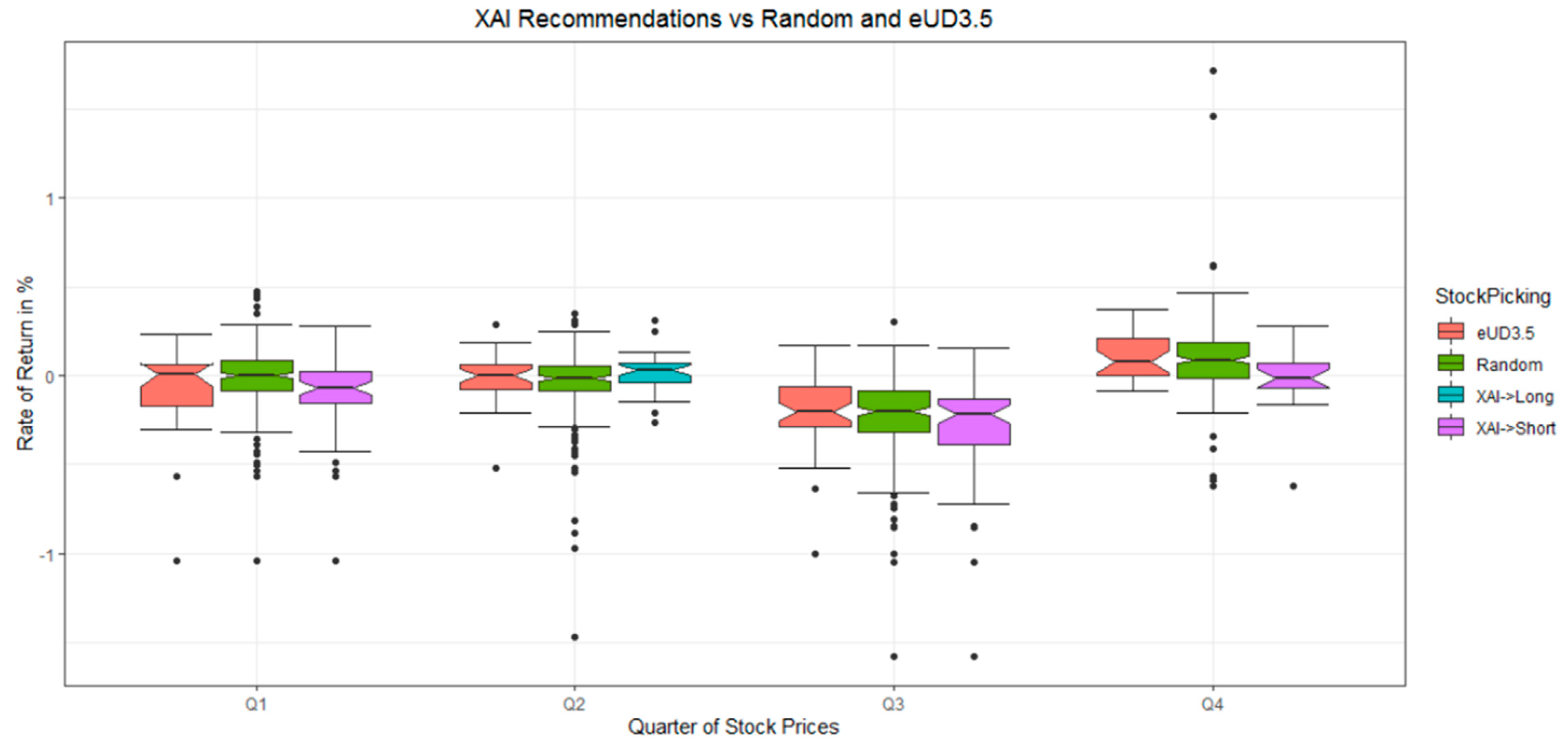
4.2. Relevance of DSD-XAI Explanations by Simulated Stock Picking

Rating the explanations of leaves leads to the hypothesis of a short or long position with stocks. For all quarters, the simulation of the picking stocks of the interesting cluster with a meaningful explanation against a random choice of stocks is shown in Table 1. Class-wise box plots of the rate of returns per company stock share and per quarter are provided in Figure 5 and allow for a more detailed view. Moreover, Figure 5 includes the evaluation of the eUD3.5 algorithm in the four quarters of the data. The eUD3.5 made it impossible to understand the explanations of a cluster and select a cluster with regard to the prediction of a short or long position for stock picking. Therefore, the small cluster of each quarter was evaluated in Figure 5 because the sizes of the clusters for each quarter were similar to the size of the selected stocks for the DSD-XAI. The success rate can be defined as the percentual difference between the random stock picking and the long/short position stock-picking of a selected class. Only the difference allows one to ignore the general trend of prices for each quarter. On average (per quarter), the success rate of the approach of this work is 25% percent higher than a random picking of stocks with an (absolute) average rate of return of 10.75%.
Therefore, it is evident that the success rate is above the chance level if the random picking of stocks sets the chance level for a short/long position. Therefore, the explanations of DSD-XAI are relevant. The stock picking based on eUD3.5 is comparable to chance and, hence, not applicable.

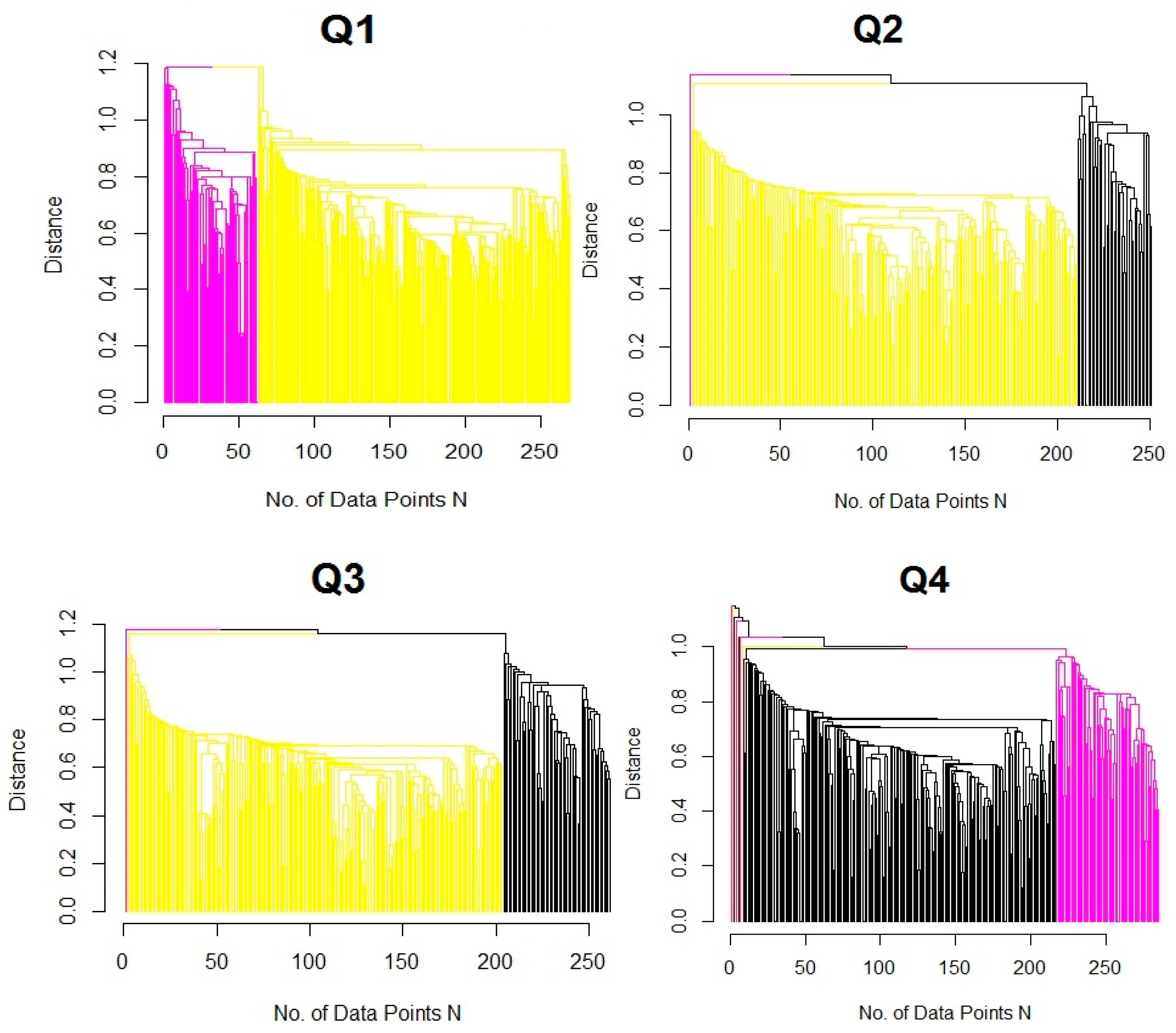
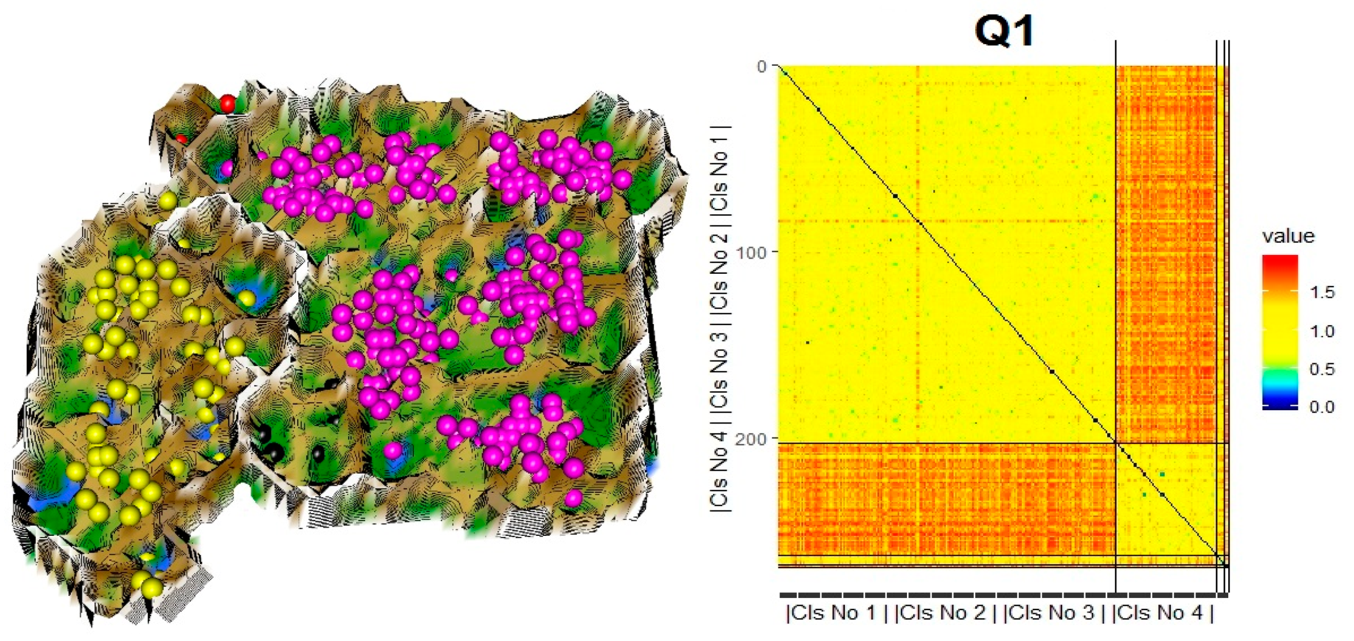
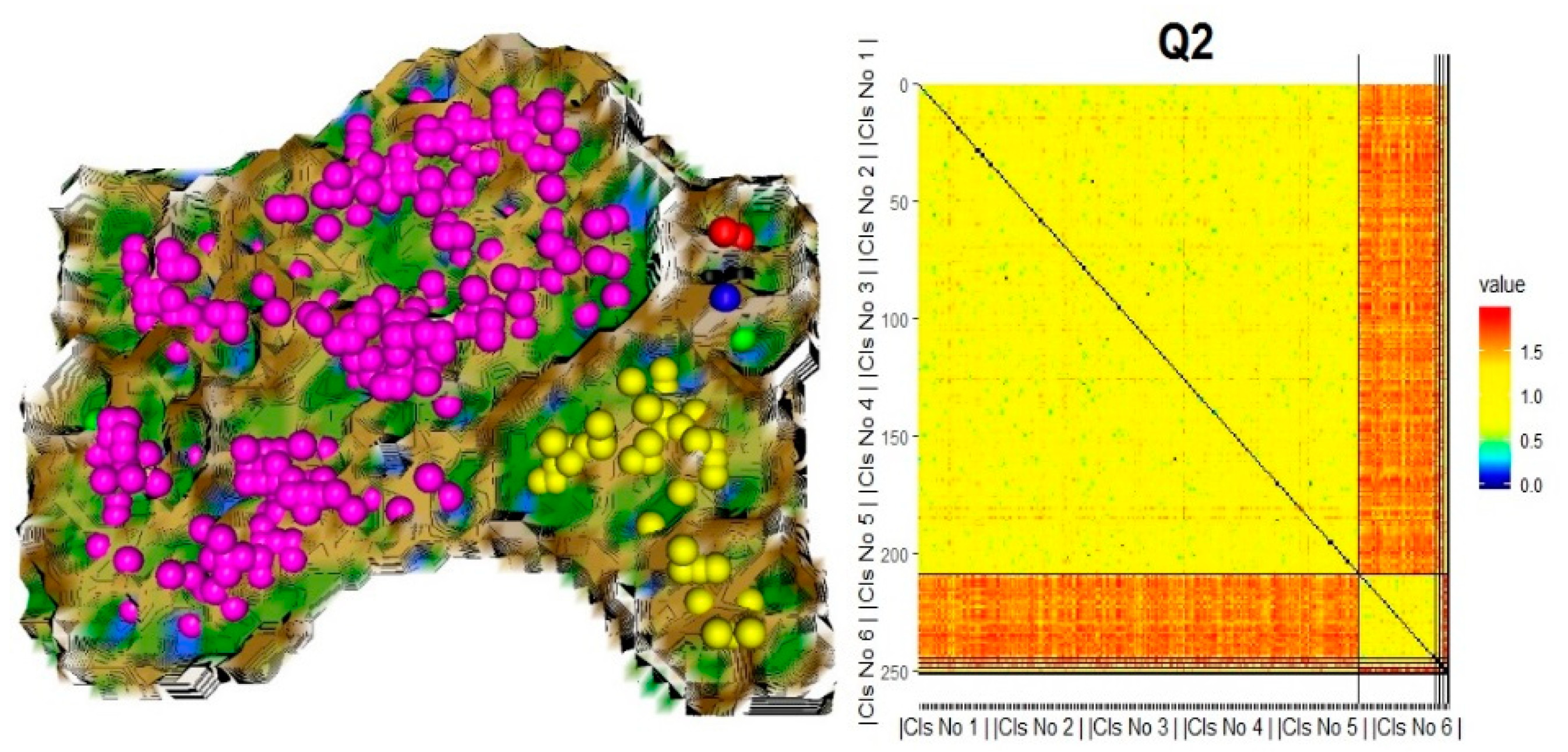
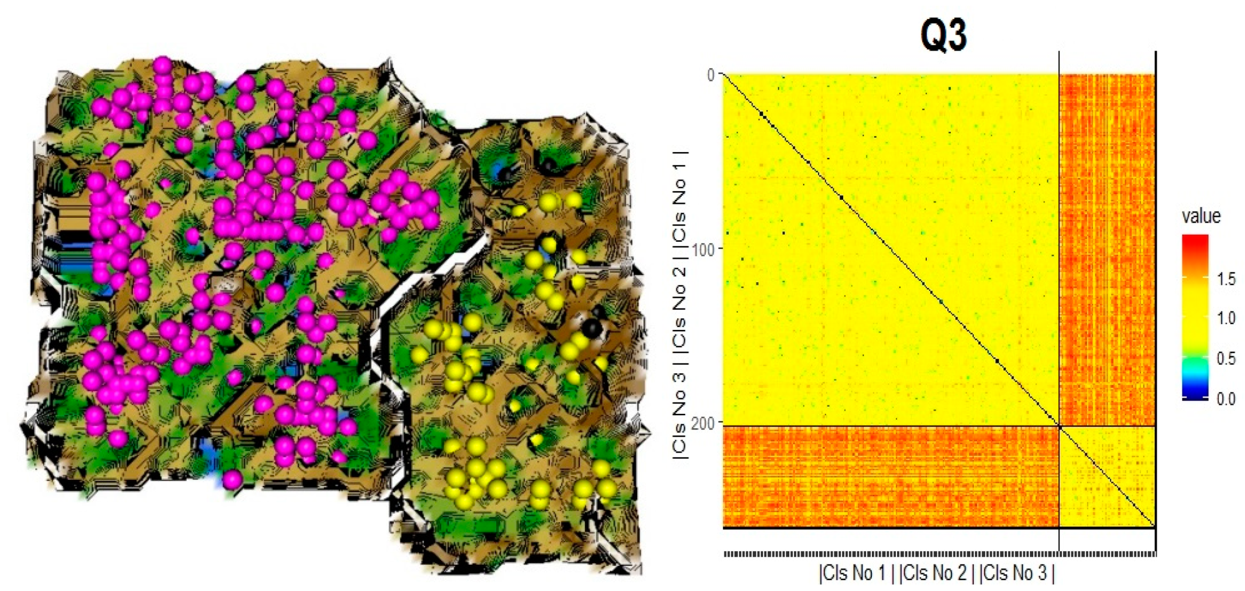
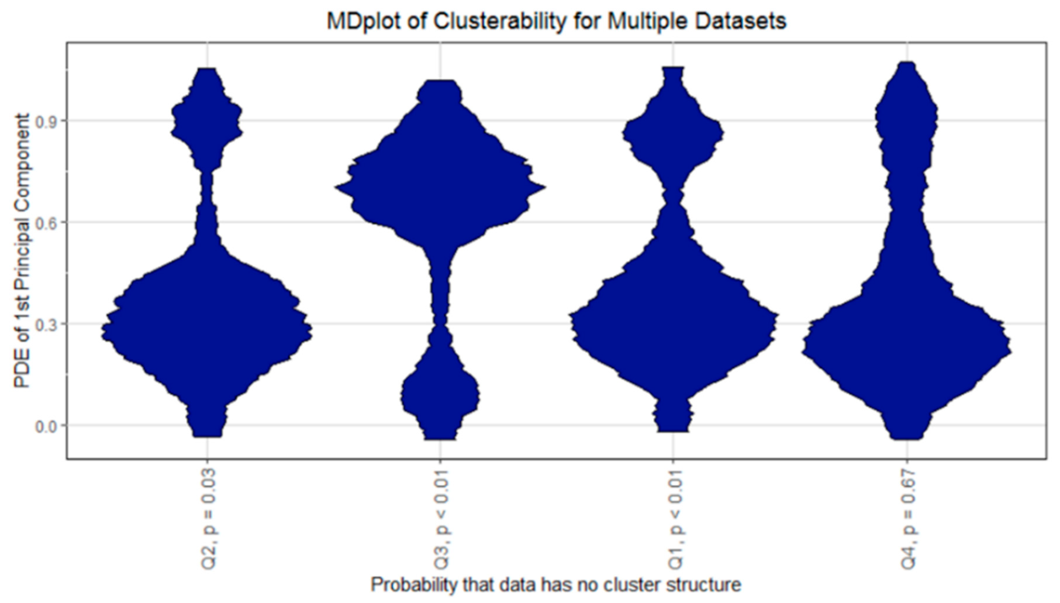
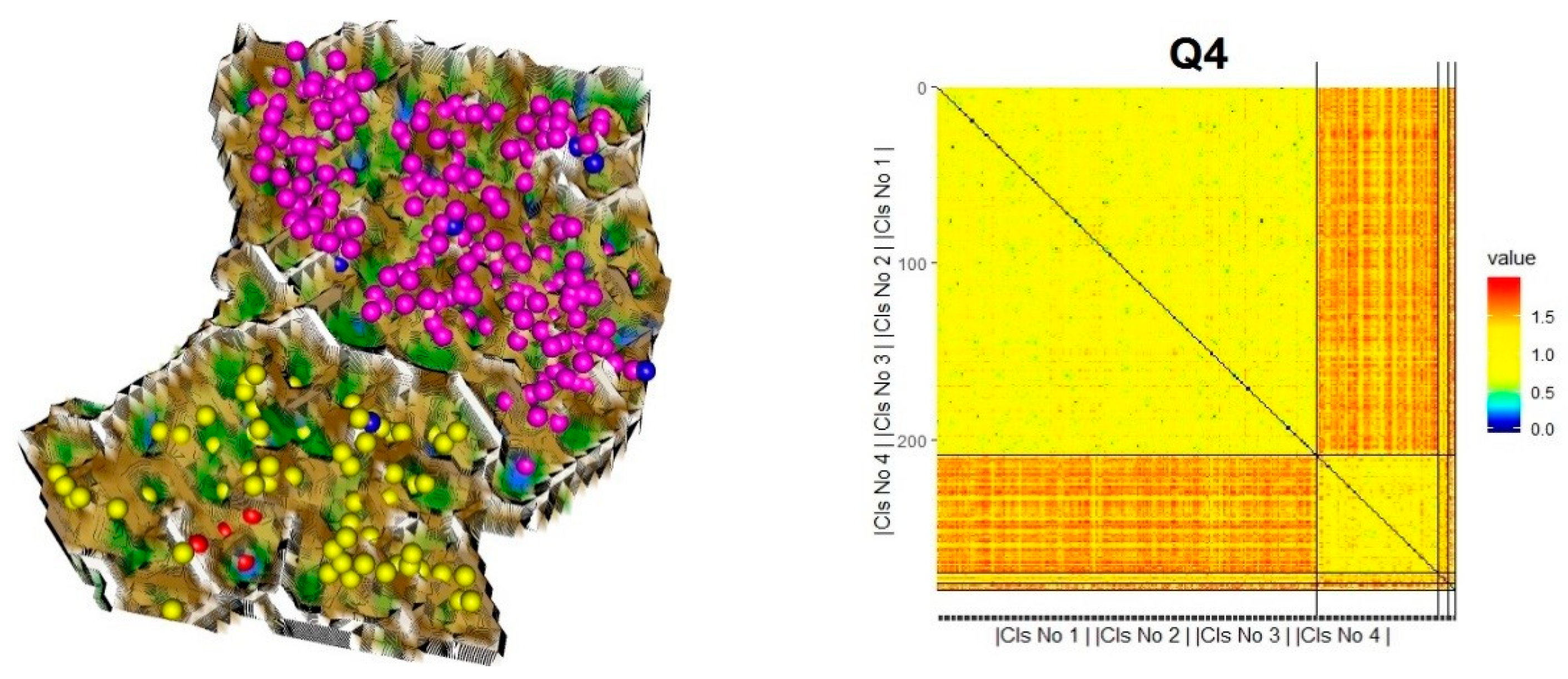
4.3. DSD Identification by Cluster Analysis and Validation

The data shows a high cluster tendency (Figure 6). Statistical testing largely agrees with density estimation that the 1st principal component is multimodal, indicating strong clusterability. For the fourth quarter, density estimation using the PDE [66] is more sensitive to multimodality than statistical testing with the dip test [41]. The dendrogram with the most significant change in the fusion levels defines the initial clustering (see Figure 7). During the clustering validation, outliers are marked interactively in the topographic maps as follows. First, the high-dimensional structures of companies’ accounting information are visible in the topographic maps per quarter in Figure 8, Figure 9, Figure 10 and Figure 11 on the left side. The points in the visualizations represent the companies. The color of the points represents the clustering. In each left figure, two valleys can be identified with several volcanos, indicating outliers resulting in three groups of data (big, small, and outliers). Second, the heatmaps on the right of Figure 8, Figure 9, Figure 10 and Figure 11 indicate the clusters are homogenous because intercluster distances are higher than intracluster distances. The distances are ordered accordingly to the provided projection-based clustering.

5. Discussion

The fundamental data used in this work did not have a classification resulting in to consequences. First, the evaluation of performance has to be based on the expected stock picking in the next respective quarter (Table 1) and compared to unsupervised XAIs. Second, the usual supervised methods, e.g., hybrid deep learning approaches or combinations with post-hoc explainers [67], were not applicable. Recently, unsupervised deep learning methods were proposed, although it is questionable based on the current literature review if such methods can reproduce structures in data better than state-of-the-art algorithms [47].
The DSD-XAI proposed here has three major advantages compared to the latest unsupervised decision trees. First, comparable approaches are limited to either use transformed data that cannot provide meaningful explanations to the domain expert or to use non-transformed data. The latter poses the issue that the usage of many distance metrics, including the most-often used Euclidean metric, requires to account for correlations (e.g., [64,68]) and the normalization of the data to avoid undesired emphasis of features with large ranges and variances [69] (see also [70]), which will lead to inappropriate clustering and therefore explanations.
Exemplarily, this issue was shown for eUD3.5 [6]. If unprocessed data is used, the eUD3.5 provides explanations for each quarter that are not meaningful and relevant based on Grice’s maxims. The eUD3.5 algorithm provides more than 400 explanations per quarter. The IMM algorithm [5] could not be compared due to the lack of source code, but using unprocessed features with the k-means or k-medoids criterion would have the same issues. It is apparent that explanations derived from unsupervised decision trees with appropriate preprocessed features would be less or not meaningful to a domain expert. In contrast, the DSD-XAI performs robustly in a high-dimensional space using preprocessed features, and a clustering-guided supervised decision tree applied to unprocessed features provides explanations around the magic number of four [58], from which stock picking is already possible.
Second, the guidance of best-performing decision trees by validated high-dimensional DSD simultaneously selects the splitting criterion of the decision tree based on actual structures in data and three out of four Grice’s maxims. Using all available features to identify DSD based on projection-based clustering has the advantage that the resulting clustering can yield novel and coherent insights through emergence [43]. In contrast, methods based on k-means or k-medoids criteria severely restrict the structures in data that can be found (e.g., [45,71]) which would hold true for the IMM algorithm.
Third, the relevance of the explanations (4th Grice’s maxim) provided by the clustering guided decision tree can be improved by selected features based on domain knowledge. The approach could be extended to the Miller optimum of 7 ± 2 if more domain knowledge about fundamental analysis is accessible.
From the perspective of domain experts, contrastive explanations, also called counterfactual explanations [72], are preferable [57]. Such counterfactual explanations tend to make future recommendations easier [67,73]. One disadvantage of this work is the fact that due to missing access to a domain expert, it could not be investigated if the presented explanations are contrastive for a non data scientist (see discussion in [61]). Hence, this work’s challenge is that only four features were—from the data scientist’s perspective—contrastive enough to decide if a stock price would go up or down (see Section 3.2). Consequently, these four features were chosen because common domain knowledge is available on the web. A rating was specified for the explanations extracted from the clustering-guided decision tree based on the four unprocessed features. Hence, domain knowledge has to specifically indicate that the selected features are not only meaningful but also relevant for stock picking. The current approach could be improved if more domain knowledge would be available, leading to a better selection of features for the decision tree.
Nevertheless, the explanations are meaningful w.r.t identified DSD of all preprocessed features. Domain knowledge allows for understanding a subset of unprocessed features used in the decision tree, enabling a rating of explanations and, hence, selecting a leaf node consisting of a subset of stocks. The explanations were relevant because they allow for stock picking of around 6–20% of available stocks. For all four quarters, even nonprofessionals in stock trading are able to conclude the price development of companies in the next quarter. Specific accounting information influences the price development of shares through the probability of a significantly higher rate of return of stock prices of companies of the selected stocks compared to random stock picking. The success rate is 25% above the chance level if the random picking of stocks sets the chance level for a short/long position.
As an alternative to using fundamental data, Gite et al. used the classification of positive and negative headlines to predict the price of an index of the Indian stock market [22] for a short period of several days. Although the error was low, no baseline was provided in their results (e.g., an LSTM model without the headlines), and no comparison to other methods were shown. In contrast, this work compares the success rate of stock picking for a long period of four quarters to the baseline of random stock picking. Such a comparison has the advantage that the volatility of the market and the central tendency of prices are mapped within the random choice of stock picking, whereas in Gite et al., it remains unclear if the seven days in the test data are only predicted accurately because of the low volatility of the market. In comparison, the success rate at stock picking by a hybrid AI system was reported with, on average, 55.19% to 60.69%, and experts had a success rate worse than chance. The eUD3.5 XAI performed similarly to random stock picking, as shown in Figure 5. Thus, the DSD-XAI approach allows data-driven stock picking with a high chance of success.

6. Conclusions

The explainable AI (XAI) approach is based on three components. First, the distance is selected, resulting in a multimodal distribution if applied to the data. Second, projection-based clustering using all and preprocessed features is applied and identifies distance-based structures in data (DSD) that are verified. Third, the DSD clustering guides the best-performing supervised decision tree of preselected and non-preprocessed features. Finally, the resulting leaves of the DSD-XAI are rated, and stocks contained in the leaf with the best rating achieve an above-average return. Consequently, stock picking based on meaningful and relevant explanations selected and assessed by the Grice maxims performs better than random stock picking, with a rate of success significantly higher than chance. Moreover, the success rate outperforms the reported success rate of two other AI systems. Contrary to other AI systems, the advantages lie in the fact that the DSD-XAI outputs are interpretable by humans, enabling them to integrate further domain experts in the stock-picking process. Additionally, the open-source code of all methods used is available.
In the future, it would be interesting to combine fundamental analysis with sentiment analysis of news headlines for stock picking. Moreover, an ensemble system in combination with technical analysis seems promising. Furthermore, it should be investigated if DSD-XAI can provide contrastive explanations to the domain expert.

Supplementary Materials

The following supporting information can be downloaded at: https://zenodo.org/deposit/5813403, Table S1: Datasets of fundamental data and stock prices. The stock prices of the same companies are always taken one quarter after the fundamental data.

Funding

This research received no external funding with the exception of the publication fee which was paid by IAP-GmbH Intelligent Analytics Projects (www.iap-gmbh.de, accessed on 20 November 2021).

Institutional Review Board Statement

Not applicable.

Informed Consent Statement

Not applicable.

Data Availability Statement

Data access of stock prices, fundamental data, and preprocessed data for the four quarters are archived on Zenodo: doi:10.5281/zenodo.5813355, accessed on 20 November 2021 under Creative Commons Attribution 3.0 Germany license.

Acknowledgments

I thank Hamza Tayyab for compiling and applying the eUD3.5 algorithm to the data and providing the web scrapping algorithm to acquire the data.

Conflicts of Interest

The authors declare no conflict of interest.

Code Availability

Specified in detail in Section 3.4.

References

  1. Breiman, L.; Friedman, J.; Stone, C.J.; Olshen, R.A. Classification and Regression Trees; CRC Press: Boca Raton, Fl, USA, 1984. [Google Scholar]
  2. Quinlan, J.R. Induction of decision trees. Mach. Learn. 1986, 1, 81–106. [Google Scholar] [CrossRef] [Green Version]
  3. Blockeel, H.; De Raedt, L.; Ramon, J. Top-down induction of clustering trees. In Proceedings of the 15th International Conference on Machine Learning, San Francisco, CA, USA, 21–27 July 1998; Shavlik, J., Ed.; Morgan Kaufmann: Burlington, MA, USA, 1998; pp. 55–63. [Google Scholar]
  4. Burkart, N.; Huber, M.F. A survey on the explainability of supervised machine learning. J. Artif. Intell. Res. 2021, 70, 245–317. [Google Scholar] [CrossRef]
  5. Dasgupta, S.; Frost, N.; Moshkovitz, M.; Rashtchian, C. Explainable K-means and K-medians clustering. In Proceedings of the 37th International Conference on Machine Learning, Virtual, 13–18 July 2020; PMLR: Vienna, Austria, 2020; pp. 7055–7065. [Google Scholar]
  6. Loyola-González, O.; Gutierrez-Rodríguez, A.E.; Medina-Pérez, M.A.; Monroy, R.; Martínez-Trinidad, J.F.; Carrasco-Ochoa, J.A.; García-Borroto, M. An Explainable Artificial Intelligence Model for Clustering Numerical Databases. IEEE Access 2020, 8, 52370–52384. [Google Scholar] [CrossRef]
  7. Thrun, M.C. The Exploitation of Distance Distributions for Clustering. Int. J. Comput. Intell. Appl. 2021, 20, 2150016. [Google Scholar] [CrossRef]
  8. Thrun, M.C.; Ultsch, A. Using projection based clustering to find distance and density based clusters in high-dimensional data. J. Classif. 2020, 38, 280–312. [Google Scholar] [CrossRef]
  9. Grice, H.P. Logic and conversation. In Speech Acts; Academic Press: New York, NY, USA, 1975; Volume 3, pp. 41–58. [Google Scholar]
  10. Thrun, M.C.; Ultsch, A.; Breuer, L. Explainable AI Framework for Multivariate Hydrochemical Time Series. Mach. Learn. Knowl. Extr. 2021, 3, 170–205. [Google Scholar] [CrossRef]
  11. Tsaih, R.; Hsu, Y.; Lai, C.C. Forecasting S&P 500 stock index futures with a hybrid AI system. Decis. Support Syst. 1998, 23, 161–174. [Google Scholar]
  12. Gelistete Unternehmen in Prime Standard, G.S.u.S. Available online: http://www.deutsche-boerse-cash-market.com/dbcm-de/instrumente-statistiken/statistiken/gelistete-unternehmen (accessed on 18 September 2018).
  13. Prime-Standard. Teilbereich des Amtlichen Marktes und des Geregelten Marktes der Deutschen Börse für Unternehmen, die Besonders hohe Transparenzstandards Erfüllen. Available online: http://deutsche-boerse.com/dbg-de/ueber-uns/services/know-how/boersenlexikon/boersenlexikon-article/Prime-Standard/2561178 (accessed on 18 September 2018).
  14. Nazário, R.T.F.; e Silva, J.L.; Sobreiro, V.A.; Kimura, H. A literature review of technical analysis on stock markets. Q. Rev. Econ. Financ. 2017, 66, 115–126. [Google Scholar] [CrossRef]
  15. Patel, J.; Shah, S.; Thakkar, P.; Kotecha, K. Predicting stock and stock price index movement using trend deterministic data preparation and machine learning techniques. Expert Syst. Appl. 2015, 42, 259–268. [Google Scholar] [CrossRef]
  16. Patel, J.; Shah, S.; Thakkar, P.; Kotecha, K. Predicting stock market index using fusion of machine learning techniques. Expert Syst. Appl. 2015, 42, 2162–2172. [Google Scholar] [CrossRef]
  17. O'Neil, W.J. How to Make Money in Stocks; McGraw-Hill: New York, NY, USA, 1988. [Google Scholar]
  18. Deboeck, G.J.; Ultsch, A. Picking stocks with emergent self-organizing value maps. Neural Netw. World 2000, 10, 203–216. [Google Scholar]
  19. Mohanram, P.S. Separating winners from losers among lowbook-to-market stocks using financial statement analysis. Rev. Account. Stud. 2005, 10, 133–170. [Google Scholar] [CrossRef]
  20. Ou, J.A.; Penman, S.H. Financial statement analysis and the prediction of stock returns. J. Account. Econ. 1989, 11, 295–329. [Google Scholar] [CrossRef]
  21. Richardson, S.; Tuna, I.; Wysocki, P. Accounting anomalies and fundamental analysis: A review of recent research advances. J. Account. Econ. 2010, 50, 410–454. [Google Scholar] [CrossRef]
  22. Gite, S.; Khatavkar, H.; Kotecha, K.; Srivastava, S.; Maheshwari, P.; Pandey, N. Explainable stock prices prediction from financial news articles using sentiment analysis. PeerJ Comput. Sci. 2021, 7, e340. [Google Scholar] [CrossRef]
  23. Ribeiro, M.T.; Singh, S.; Guestrin, C. “Why should I trust you?” Explaining the predictions of any classifier. In Proceedings of the 22nd ACM SIGKDD International Conference on Knowledge Discovery and Data Mining, San Francisco, CA, USA, 13–17 August 2016; pp. 1135–1144. [Google Scholar]
  24. Ultsch, A. The integration of connectionist models with knowledge-based systems: Hybrid systems. In Proceedings of the SMC'98 Conference Proceedings, 1998 IEEE International Conference on Systems, Man, and Cybernetics (Cat. No.98CH36218), San Diego, CA, USA, 14 October 1998; IEEE: San Diego, CA, USA, 1998; pp. 1530–1535. [Google Scholar]
  25. Lundberg, S.M.; Lee, S.-I. A unified approach to interpreting model predictions. In Proceedings of the 31st International Conference on Neural Information Processing Systems 2017, Long Beach, CA, USA, 4–9 December 2017; pp. 4765–4774. [Google Scholar]
  26. Ultsch, A.; Korus, D. Integration of neural networks and knowledge-based systems. In Proceedings of the International Conference on Neural Networks, Perth, Australia, 27 November–1 December 1995; IEEE: Perth, Australia, 1995; pp. 1–6. [Google Scholar]
  27. Biran, O.; Cotton, C. Explanation and justification in machine learning: A survey. In IJCAI-17 Workshop Explainable AI (XAI); IJCAI: Macao, SA, USA, 2017; pp. 8–13. [Google Scholar]
  28. Adadi, A.; Berrada, M. Peeking inside the black-box: A survey on Explainable Artificial Intelligence (XAI). IEEE Access 2018, 6, 52138–52160. [Google Scholar] [CrossRef]
  29. Lipton, Z.C. The mythos of model interpretability. Queue 2018, 16, 31–57. [Google Scholar] [CrossRef]
  30. Ultsch, A.; Halmans, G.; Mantyk, R. CONKAT: A connectionist knowledge acquisition tool. In Proceedings of the 24th Annual Hawaii International Conference on System Sciences, Kauai, HI, USA, 8–11 January 1991; IEEE: Kauai, HI, USA, 1991; pp. 507–513. [Google Scholar]
  31. Ultsch, A.; Korus, D.; Kleine, T. Integration of neural networks and knowledge-based systems in medicine. In Proceedings of the Conference on Artificial Intelligence in Medicine in Europe, Pavia, Italy, 25–28 June 1995; Barahona, P., Stefanelli, M., Wyatt, J., Eds.; Springer: Berlin, Heidelberg, 1995; pp. 425–426. [Google Scholar]
  32. Letham, B.; Rudin, C.; McCormick, T.H.; Madigan, D. An interpretable stroke prediction model using rules and bayesian analysis. In Proceedings of the 17th AAAI Conference on Late-Breaking Developments in the Field of Artificial Intelligence, Bellevue, WD, USA, 14–18 July 2013; AAAI Press: New York, NY, USA, 2013; pp. 65–67. [Google Scholar]
  33. Riid, A.; Sarv, M. Determination of regional variants in the versification of estonian folksongs using an interpretable fuzzy rule-based classifier. In Proceedings of the 8th Conference of the European Society for Fuzzy logic and Technology (EUSFLAT-13), Milano, Italy, 11–13 September 2013; Atlantis Press: Amsterdam, The Netherlands, 2013; pp. 61–66. [Google Scholar]
  34. Nauck, D.; Kruse, R. Obtaining interpretable fuzzy classification rules from medical data. Artif. Intell. Med. 1999, 16, 149–169. [Google Scholar] [CrossRef]
  35. Lakkaraju, H.; Bach, S.H.; Leskovec, J. Interpretable decision sets: A joint framework for description and prediction. In Proceedings of the 22nd ACM SIGKDD International Conference on Knowledge Discovery and Data Mining, San Francisco, CA, USA, 13–17 August 2016; IEEE: New York, NY, USA, 2016; pp. 1675–1684. [Google Scholar]
  36. Hewett, R.; Leuchner, J. The power of second-order decision tables. In Proceedings of the 2nd SIAM International Conference on Data Mining, Arlington, VA, USA, 11–13 April 2002; SIAM: New Delhi, India, 2002; pp. 384–399. [Google Scholar]
  37. Dehuri, S.; Mall, R. Predictive and comprehensible rule discovery using a multi-objective genetic algorithm. Knowl. Based Syst. 2006, 19, 413–421. [Google Scholar] [CrossRef]
  38. Basak, J.; Krishnapuram, R. Interpretable hierarchical clustering by constructing an unsupervised decision tree. IEEE Trans. Knowl. Data Eng. 2005, 17, 121–132. [Google Scholar] [CrossRef]
  39. Kim, B.; Shah, J.A.; Doshi-Velez, F. Mind the gap: A generative approach to interpretable feature selection and extraction. In Proceedings of the 28th International Conference on Neural Information Processing Systems, Montreal, QC, Canada, 7–12 December 2015; MIT Press: Cambridge, MA, USA, 2015; pp. 2260–2268. [Google Scholar]
  40. Thrun, M.C.; Gehlert, T.; Ultsch, A. Analyzing the Fine Structure of Distributions. PLoS ONE 2020, 15, e0238835. [Google Scholar] [CrossRef]
  41. Hartigan, J.A.; Hartigan, P.M. The dip test of unimodality. Ann. Stat. 1985, 13, 70–84. [Google Scholar] [CrossRef]
  42. Orloci, L. An agglomerative method for classification of plant communities. J. Ecol. 1967, 55, 193–206. [Google Scholar] [CrossRef] [Green Version]
  43. Thrun, M.C.; Ultsch, A. Swarm intelligence for self-organized clustering. Artif. Intell. 2021, 290, 103237. [Google Scholar] [CrossRef]
  44. Van der Merwe, D.; Engelbrecht, A.P. Data clustering using particle swarm optimization. In Proceedings of the Evolutionary Computation, CEC'03, Canberra, Australia, 8–12 December 2003; IEEE: Canberra, Australia, 2003; pp. 215–220. [Google Scholar]
  45. Thrun, M.C. Projection Based Clustering through Self-Organization and Swarm Intelligence; Ultsch, A., Hüllermeier, E., Eds.; Springer: Heidelberg, Germany, 2018. [Google Scholar] [CrossRef] [Green Version]
  46. Ultsch, A.; Lötsch, J. Machine-learned cluster identification in high-dimensional data. J. Biomed. Inform. 2017, 66, 95–104. [Google Scholar] [CrossRef] [PubMed]
  47. Thrun, M.C. Distance-Based Clustering Challenges for Unbiased Benchmarking Studies. Nat. Sci. Rep. 2021, 11, 18988. [Google Scholar] [CrossRef]
  48. Murtagh, F. On ultrametricity, data coding, and computation. J. Classif. 2004, 21, 167–184. [Google Scholar] [CrossRef]
  49. Adolfsson, A.; Ackerman, M.; Brownstein, N.C. To cluster, or not to cluster: An analysis of clusterability methods. Pattern Recognit. 2019, 88, 13–26. [Google Scholar] [CrossRef] [Green Version]
  50. Ahmed, M.O.; Walther, G. Investigating the multimodality of multivariate data with principal curves. Comput. Stat. Data Anal. 2012, 56, 4462–4469. [Google Scholar] [CrossRef]
  51. Thrun, M.C. Improving the sensitivity of statistical testing for clusterability with mirrored-density plot. In Machine Learning Methods in Visualisation for Big Data; Archambault, D., Nabney, I., Peltonen, J., Eds.; The Eurographics Association: Norrköping, Sweden, 2020; pp. 1–17. [Google Scholar]
  52. Thrun, M.C.; Ultsch, A. Uncovering High-Dimensional Structures of Projections from Dimensionality Reduction Methods. MethodsX 2020, 7, 101093. [Google Scholar] [CrossRef]
  53. Thrun, M.C.; Lerch, F.; Lötsch, J.; Ultsch, A. Visualization and 3D printing of multivariate data of biomarkers. In Proceedings of the International Conference in Central Europe on Computer Graphics, Visualization and Computer Vision, Plzen, Czech Republic, 30 May–3 June 2016; Skala, V., Ed.; WSCG: Plzen, Czech Republic, 2016; pp. 7–16. [Google Scholar]
  54. Dasgupta, S.; Gupta, A. An elementary proof of a theorem of Johnson and Lindenstrauss. Random Struct. Algorithms 2003, 22, 60–65. [Google Scholar] [CrossRef]
  55. Johnson, W.B.; Lindenstrauss, J. Extensions of lipschitz mappings into a hilbert space. Contemp. Math. 1984, 26, 189–206. [Google Scholar] [CrossRef]
  56. Silver, C.; Chen, J.; Hong, E.; Kagan, J.; Kenton, W.; Krishna, M. Operating Income; Investopedia LLC: New York, NY, USA, 2014. [Google Scholar]
  57. Miller, T. Explanation in artificial intelligence: Insights from the social sciences. Artif. Intell. 2019, 267, 1–38. [Google Scholar] [CrossRef]
  58. Cowan, N. The magical number 4 in short-term memory: A reconsideration of mental storage capacity. Behav. Brain Sci. 2001, 24, 87–114. [Google Scholar] [CrossRef] [Green Version]
  59. Miller, G.A. The magical number seven, plus or minus two: Some limits on our capacity for processing information. Psychol. Rev. 1956, 101, 343–352. [Google Scholar] [CrossRef]
  60. Mörchen, F.; Ultsch, A.; Hoos, O. Extracting interpretable muscle activation patterns with time series knowledge mining. Int. J. Knowl. Based Intell. Eng. Syst. 2005, 9, 197–208. [Google Scholar] [CrossRef] [Green Version]
  61. Miller, T.; Howe, P.; Sonenberg, L.; AI, E. Explainable AI: Beware of inmates running the asylum. In IJCAI 2019 Workshop on Explainable Artificial Intelligence (XAI); IJCAI: Melbourne, Australia, 2017; pp. 36–42. [Google Scholar]
  62. Ultsch, A. Is Log Ratio a Good Value for Measuring Return in Stock Investments? In Advances in Data Analysis, Data Handling and Business Intelligence; Springer: Berlin/Heidelberg, Germany, 2009; pp. 505–511. [Google Scholar]
  63. Welch, B.L. The significance of the difference between two means when the population variances are unequal. Biometrika 1938, 29, 350–362. [Google Scholar] [CrossRef]
  64. Cormack, R.M. A review of classification. J. Roy. Stat. Soc. Ser. A (Gen.) 1971, 134, 321–367. [Google Scholar] [CrossRef]
  65. Grubinger, T.; Zeileis, A.; Pfeiffer, K.-P. evtree: Evolutionary learning of globally optimal classification and regression trees in R. J. Stat. Softw. 2014, 61, 1–29. [Google Scholar] [CrossRef] [Green Version]
  66. Ultsch, A. Pareto density estimation: A density estimation for knowledge discovery. In Innovations in Classification, Data Science, and Information Systems; Baier, D., Werrnecke, K.D., Eds.; Springer: Berlin, Germany, 2005; pp. 91–100. [Google Scholar]
  67. Joshi, G.; Walambe, R.; Kotecha, K. A Review on Explainability in Multimodal Deep Neural Nets. IEEE Access 2021, 9, 59800–59821. [Google Scholar] [CrossRef]
  68. Mimmack, G.M.; Mason, S.J.; Galpin, J.S. Choice of distance matrices in cluster analysis: Defining regions. J. Clim. 2001, 14, 2790–2797. [Google Scholar] [CrossRef]
  69. Mörchen, F. Time Series Knowledge Mining; Citeseer/Görich & Weiershäuser: Marburg, Germany, 2006. [Google Scholar]
  70. Jain, A.K.; Dubes, R.C. Algorithms for clustering data. In Prentice Hall Advanced Reference Series: Computer Science; Marttine, B., Ed.; Prentice Hall: Englewood Cliffs, NJ, USA, 1988; pp. 1–320. [Google Scholar]
  71. Hennig, C.; Meila, M.; Murtagh, F.; Rocci, R. Handbook of cluster analysis. In Handbook of Modern Statistical Methods; Hennig, C., Meila, M., Murtagh, F., Rocci, R., Eds.; Chapman & Hall/CRC Press: New York, NY, USA, 2015; pp. 1–730. [Google Scholar]
  72. Wachter, S.; Mittelstadt, B.; Russell, C. Counterfactual explanations without opening the black box: Automated decisions and the GDPR. Harv. JL Tech. 2017, 31, 841. [Google Scholar] [CrossRef] [Green Version]
  73. Karimi, A.-H.; Schölkopf, B.; Valera, I. Algorithmic recourse: From counterfactual explanations to interventions. In Proceedings of the 2021 ACM Conference on Fairness, Accountability, and Transparency, Virtual Event, 3–10 March 2021; pp. 353–362. [Google Scholar]
Figure 1. Decision tree using evolutionary learning of globally optimal trees [65] with an overall accuracy of 91% of the projection-based clustering of the fourth quarter. The left-most path is selected because the path has the highest absolute rating. The hypothesis is to select these 17 stocks for a short position for the first quarter of the next year.
Information 13 00051 g001
Figure 2. Decision tree using evolutionary learning of globally optimal trees with an overall accuracy of 93% of the clustering of the first quarter based on the DSD. The left-most path is selected because the path has the highest absolute rating. The hypothesis is to select these 59 stocks for a short position in the second quarter.
Information 13 00051 g002
Figure 3. Decision tree using evolutionary learning of globally optimal trees with an overall accuracy of 96% of the clustering of the second quarter based on the DSD. The right-most path is selected because the path has the highest absolute rating. The hypothesis is to select these 36 stocks for a long position in the third quarter.
Information 13 00051 g003
Figure 4. Decision tree using evolutionary learning of globally optimal trees with an overall accuracy of 96% of the clustering of the third quarter based on the DSD. The left-most path is selected because the path has the highest absolute rating. The hypothesis is to select these 56 stocks for a short position for the fourth quarter.
Information 13 00051 g004
Figure 5. Class wise box plot of the rate of return in % calculated with relative differences [62] per investigated Quarter. “XAI->Long” or “XAI->short” are the interpreted explanations for which the stocks were purchased in either short or long sales. Stock picking is conducted consistently in the quarter following the cluster analysis. The difference between random and the DSD-XAI stock-picking is statistically significant but between random and eUD3.5 is not. All features shown in the boxplots were tested with the dip test against multimodality, yielding non-significant p-values.
Information 13 00051 g005
Figure 6. The evaluation of cluster tendency using the method described in [51] shows a high clusterability because multimodality is visible in all four quarters. Moreover, statistical testing agrees for the first three quarters that the distribution of the 1st principal component is multimodal.
Information 13 00051 g006
Figure 7. Dendrograms show that the projection-based clustering is performed at the most remarkable change in the fusion levels of the branches in the dendrograms. The dendrograms of the quarters are ordered from Q1 to Q4.
Information 13 00051 g007
Figure 8. The topographic map (left) visualizes high-dimensional, distance-based structures in data (DSD) by separating clusters through watersheds of mountains. It shows two valleys for the companies (points) of the first quarter—one primary cluster with companies labeled with the color magenta, one smaller cluster with companies labeled in yellow, and various outliers (black and red). Heatmap indicates an appropriate clustering because intracluster distances are smaller (in yellow) than intercluster distances (orange).
Information 13 00051 g008
Figure 9. For the accounting information of the second quarter, the topographic map shows DSD in two valleys—one primary cluster with companies represented by magenta points, one smaller cluster with companies in yellow, and various outliers (other colors). Heatmap indicates an appropriate clustering because intracluster distances are smaller (in yellow) than intercluster distances (orange).
Information 13 00051 g009
Figure 10. For the accounting information of the third quarter, the topographic map shows DSD in two valleys—one primary cluster with companies represented by magenta points (one smaller cluster with companies in yellow and various outliers (black). Heatmap indicates an appropriate clustering because intracluster distances are smaller (in yellow) than intercluster distances (orange).
Information 13 00051 g010
Figure 11. For the accounting information of the fourth quarter, the topographic map shows DSD in two valleys—one primary cluster with companies represented by magenta points, one smaller cluster with companies in yellow, and various outliers (red and black colors). Heatmap indicates an appropriate clustering because intracluster distances are smaller (in yellow) than intercluster distances (orange).
Information 13 00051 g011
Table 1. Backtesting of the rate of success if picked stocks were bought at the beginning of the respective quarter and sold at the end of the quarter. Stock picking by DSD-XAI is compared against random picking. More detailed statistical information is provided in Figure 5. Hartigan and Hartigan [41] dip tests against multimodality and one-sided t-tests [63] random versus selected class were performed.
Quarter
Cluster Analysis
Quarter of
Stock Prices
Price Development of Selected Stocks in DSD-XAIRandomRate of Success
(Significance of t-Test)
2018, Q42019, Q161% of stocks fall with an average rate of return of −8%51% of stocks fall with an average rate of return of −1%10%
p ( t = 2.3 , d f = 69.92 ) < 0.012
2018, Q12018, Q257% of stocks rise with an average rate of return of 2%43% of stocks rise with an average rate of return of −4 %14%
p ( t = 2.47 , d f = 66 ) = 0.008
2018, Q22018, Q395% of stocks fall with an average rate of return of −31%91% of stocks fall with an average rate of return of −22%4% with
p ( t = 1.89 , d f = 70.26 ) = 0.03
2018, Q32018, Q452% of stocks fall with an average rate of return of −2%30% of stocks fall with an average rate of return of 9%22% with
p ( t = 2.3 , d f = 18.38 ) = 0.02
Publisher’s Note: MDPI stays neutral with regard to jurisdictional claims in published maps and institutional affiliations.

