Abstract
We study classes of geometric graphs, which all correspond to the following structural characteristic. For each instance of a vertex set drawn from a universe of possible vertices, each pair of vertices is either required to be connected, forbidden to be connected, or existence or non-existence of an edge is undetermined. The conditions which require or forbid edges are universally quantified predicates defined over the vertex pair, and optionally over existence or non-existence of another edge originating at the vertex pair. We consider further a set of simple graph transformations, where the existence of an edge between two vertices is logically determined by the existence or non-existence of directed edges between both vertices in the original graph. We derive and prove the correctness of a logical expression, which is a necessary and sufficient condition for containedness relations between graph classes that are described this way. We apply the expression on classes of geometric graphs, which are used as theoretical wireless network graph models. The models are constructed from three base class types and intersection combinations of them, with some considered directly and some considered as symmetrized variants using two of the simple graph transformations. Our study then goes systematically over all possible graph classes resulting from those base classes and all possible simple graph transformations. We derive automatically containedness relations between those graph classes. Moreover, in those cases where containedness does not hold, we provide automatically derived counter examples.
1. Introduction
In this paper, we study, for a specific type of axiomatically described graph, how to prove containedness between geometric graph classes automatically. The term graph class here means a collection of graphs that satisfy the same property. Specifically, a geometric graph class refers to graphs with vertices drawn in the Euclidean space, or more generally, in a metric space. Given two graph classes, proving containedness refers to checking whether one class is contained in the other, i.e., any graph from one class is also a valid graph in the other class.
The studied method to prove containedness is illustrated with simple geometric graph models used in the theoretical wireless network research. The method in general is applicable to any geometric graph class, which can be described using a class of axioms containing inclusion conditions, which enforce the existence of an edge between two vertices, exclusion conditions, which prohibit the existence of an edge between two vertices and transfer conditions, which enforce the existence of edges between two vertices depending on the existence of other edges originating from the two vertices to be connected. The axioms depend on properties of the two vertices (inclusion; exclusion) or the three vertices (transfer) but not on the remaining vertices of the vertex set. For any two vertices where neither an edge is enforced or prohibited by the inclusion, exclusion, or transfer conditions, we are free to choose to connect them by an edge or not.
In addition to the graph classes themselves, we also examine graph transformations on graph classes. A transformation is a mapping that constructs a new graph from a given graph on the basis of logical rules applied on edge and vertex properties. More specifically, we consider transformations on graph classes, which we call simple. A simple transformation maps a source graph on an image graph with the same vertex set. The existence or nonexistence of an edge between two vertices in the image graph depends on the existence or nonexistence of the two possible edges between the two vertices in the source graph. Such dependencies can be described using Boolean expressions with two variables.
This work is an extension of our previous work [1], where we studied, with symmetric subgraph and symmetric supergraph, two specific simple transformations. In general, with two edges either existing or not existing, there are 16 simple transformations. In this work, we define those 16 transformations and systematically study all of them by automatically proving containedness relations between all possible classes resulting from specific inclusion, exclusion and transfer axioms and all possible transformations applied on these classes. More precisely, given two graph classes , , which can be described using inclusion, exclusion, and transfer axioms, let and be the classes obtained by applying the simple graph transformations, and . We test automatically whether class is contained in class . The test yields satisfiability if the subclass relation holds. Otherwise, if not, the test yields a vertex minimal example graph, which is contained in but not in .
The studied problem is not trivial. On the one hand, the predicates used for enforcing resp. prohibiting edges can be themselves formulas in a complex theory (in which properties or norms, costs or distances need to be specified). On the other hand, consider the question whether a class is contained in a class obtained from class after applying a (simple) transformation . To answer this question, one would typically need to demonstrate that for every graph H in class , there exists a graph G in class , such that , or to give an example of a graph H in , such that for every graph G in , we have . A naive logical encoding of such properties would require quantification over binary relations. In order to avoid these problems, in this paper we demonstrate how expressions (involving only the predicates for enforcing and prohibiting edges and for transfer) for testing containedness between graph classes can be generated in a systematic way. For this, we prove a small model theorem. Our results can be regarded as a form of second-order quantifier elimination [2,3].
In summary, the contributions of this work are: (1) We systematically describe geometric wireless network graph classes on the basis of so-called inclusion, exclusion, and transfer predicates. (2) By means of the so-called simple graph transformations applied on these classes, we cover additional graph classes, with some of them also considered to describe geometric wireless network graphs. (3) We derive a logical formula to automatically verify whether one of such graph clasess described by inclusion, exclusion, and transfer predicates and simple graph transformations is contained in another one or not. (4) The result is used to systematically investigate all possible containedness relations of the so-defined classes, demonstrating all possible combinations in a table at the end of this paper. (5) Finally, for those pairs of classes where containment does not hold, an automatically generated minimal counter example is provided.
The remainder of the paper is structured as follows. In the next section, we illustrate the concept of the considered graph classes and transformations with an example referring to graph models used in theoretical wireless network research. In Section 3, we formally introduce the terminology, in particular, notions such as inclusion, exclusion and transfer axioms and graph classes defined with these types of axioms, as well as the notion of simple transformations. In Section 4, we propose a method of generating finite axiomatizations for a class , which do not refer to the edges of graphs in . Furthermore, we prove a small model theorem (i.e., we demonstrate that searching for a counter example with at most four vertices is sufficient for checking containedness relations for the graph classes and transformations that we study in this paper). We use this for reducing subclass relationship tests to check the satisfiability of expressions (built in a systematic way), which do not refer to the edges of the graphs but only to the inclusion, exclusion and transfer predicates used in the description of the classes. Based on these results, we demonstrate in Section 5 how containedness relations can be proved for the 128 possible graph classes resulting from the examples discussed in Section 2. We conclude this contribution in Section 6 and discuss future research directions on extending the concept of logical graph class definitions and the concept of logical described transformations. The paper is accompanied with three appendices. Appendices Appendix A and Appendix B demonstrate an automatically derived table of the containedness relations between all 128 possible graph classes, as well as the automatically found minimal graph examples for those cases where containedness does not hold. Appendix C finally provides a longer proof for a technical lemma used for the axiomatization of the studied graph transformations.
2. Geometric Graph Models
We illustrate our theory with graph models applied in the theoretical wireless network research. Initial theoretical studies modeled such networks as unit disk graphs , where network vertices are connected if their Euclidean distance is less or equal than 1 and vertices are not connected by self-loops. The model was extended in several directions. We consider the extensions quasi units disk graphs [4,5] and directed transmission graphs [6,7,8] (Note, we consider a maximum communication distance of 1. This is no limitation to other work, where a maximum communication distance is used instead. Obviously, scaling vertex positions with yields the same model with maximum communication distance 1).
Quasi unit disk graphs have a maximum distance 1 and a minimum distance . Two distinct vertices with a Euclidean distance less or equal r are always connected. Two vertices with Euclidean distance greater than 1 are never connected. Any other vertex pairs can be but do not have to be connected. To our knowledge, quasi unit disk graphs have only been studied as undirected graphs. We assume here as well that they are undirected graphs when we speak of quasi unit disk graphs.
With directed transmission graphs , every vertex v has an individual maximum communication distance for some general . A directed edge exists from v to w if the distance between v and w is less or equal to . Directed transmission graphs can be made symmetric by removing all directed edges where the reverse edge is missing, as described in [6,9] or by adding the missing reverse edges, as it is additionally considered in [6]. We denote these graphs by and , respectively.
In the following, we describe the defining properties of the discussed graph models in terms of three base graph classes and the two discussed basic graph transformations, i.e., either removing directed edges where the reverse edge is missing or adding the missing reverse edges.
Definition 1
(The classes , , ). Let . We consider a graph . Let be any metric defined on the vertices (e.g., Euclidean distance when vertices are located in the Euclidean space). Let be if and ; otherwise, graph G is in the class of min disk graphs , max disk graphs , or connected region graphs if it satisfies the following corresponding conditions:
Definition 2
(Symmetric super and subgraph). Given a graph , the graph transformations and , denoted as symmetric supergraph and symmetric subgraph, respectively, are defined by:
When applied on a whole graph class , we write , which means that the transformation γ is applied on each graph contained in .
Obviously, the graph class of unit disk graphs can be built from the defined base classes, as follows
where intersection ∩ means that the graph is contained in both classes, or expressed alternatively, has to satisfy the logical predicates of both classes.
Together with the two basic graph transformations, the class of quasi unit disk graphs [4,5] is given by
The latter equality holds, since an edge is optional if is optional, i.e., . Obviously, is the special case of unit disk graphs .
The class of directed transmission graphs [6,7,8] is given by
This is followed immediately by setting the individual maximum communication distance of vertex v to . The symmetric variant considered in [9] has no maximum communication distance and is obtained by removing all directed edges where the reverse edge is missing. It is thus described by . The symmetric variants considered in [6] are and in our graph class notation.
3. Axiomatic Description of Graph Classes
3.1. Inclusion, Exclusion, and Transfer Predicates
Generally speaking, in the motivating example, we consider graph classes , where each graph consists of vertices V of a vertex universe and an edge relation E, which satisfies
We term , and inclusion, exclusion, and transfer predicates, respectively. We will refer to the Conditions (1)–(3) as inclusion, exclusion and transfer axioms, accordingly (though Conditions (3) and (4) are equivalent, we list both here for later reference).
We say that a graph is in class (and write ) if G satisfies the Conditions (1)–(3). In this case, we sometimes also write Gsatisfies class . If the graph class C consists of all graphs satisfying a set of axioms of the form (1)–(3), we will say that C is a graph class described by inclusion, exclusion, and transfer axioms. In this work, we will study such graph classes and transformations on them. We make the following additional assumptions:
Assumption A1.
(Independence)We assume that the inclusion, exclusion and transfer predicates are determined by the properties of their arguments and are independent of any other vertices in V. We can ensure this, for instance, by requiring that these predicates are expressed as quantifier-free formulae over a background theory.
The inclusion, exclusion, and transfer predicates defining the classes , and in Section 2 can be expressed as quantifier-free formulas over a theory in which we can talk about points and distances between points:
Assumption A2.
(Transitivity)We assume the transfer predicates to be transitive, i.e.,
Obviously, the transfer predicate defining in Section 2 is transitive.
Assumption A3.
(Soundness)We assume inclusion, exclusion, and transitive transfer predicates to be sound, which means that they are not contradicting:
We term a graph class to be sound in this case.
It is easy to see, as long as any conjunction of the predicates , and defined in Section 2 satisfies the soundness condition.
3.2. Simple Graph Class Transformations
The most general form of a graph transformation is a mapping which transfers a given graph G into a graph H. A graph transformation applied on a graph class results in a graph class , which consists of all graphs H for which there exists a graph with .
We say a graph transformation is vertex preserving if has the same vertex set as G, i.e., given , the transformation is for some F. Obviously, a vertex preserving transformation on the null graph yields the null graph.
We term a vertex preserving graph transformation simple if there exists a Boolean function in two variables (where is the two-element Boolean algebra) such that for all graphs the transformation satisfies
The symmetric super graph and symmetric subgraph are obviously simple transformations with boolean functions ∨ and ∧, respectively. As there are possible Boolean functions of the form , in total, there exist 16 possible vertex preserving simple graph transformations, as shown in Table 1 and Table 2.

Table 1.
The eight non-negated vertex preserving simple graph transformations.
Table 2.
The eight negated vertex preserving simple graph transformations.
In both tables, all four possible combinations of existence or non-existence of the edge and in the original graph is shown in the table header by the column values 0 and 1 for and . For each of those possible cases, the edge can be added or not added to the resulting image graph. All possible combinations are shown by the eight rows of both tables (i.e., 16 in total) by the values 0 and 1 for , where defines the existence or non-existence of the edge in the resulting image graph.
We define for each transformation a symbol and a mnemonic in Table 1. For each transformation in that table, the negated form can be defined, as listed in Table 2. Given a transformation , the negated transformation yields the complement graph of the graph G resulting from , i.e., each existing edge in G is erased and each missing edge in G is added. Specifically for the transformation empty graph , the negated empty graph is the complete graph, of course.
We list in the last column of Table 1 whether the transformations always yield a symmetric graph (i.e., ), a directed graph (i.e., ), or whether we keep that column entry empty if the image graph is neither necessarily symmetric nor directed. As shown in Table 2, the symmetry is preserved for the complementary graphs given by the negated transformations. However, the last two shown transformations yield graphs, which we term complementary directed, which means that the complement of the graph is directed.
In the following discussion, we have to distinguish between the two specific transformations xor graph and as well negate the xor graph and all remaining ones. It turns out that for all cases, despite these two xor ones, a small counter example with, at most, four vertices can be found if a subclass relation does not hold. For the two xor cases, this is not the case. For these two transformations, arbitrary long chains of edge dependencies to determine minimum counter examples are possible. The proof is given in Lemma 5. Only under a specific condition (as discussed later), and also for the two xor cases, proving that a subclass relation does not hold, is possible with a four vertex example.
To distinguish between those situations where all transformation are considered and where all despite the two xor cases are considered, we define for the following discussion by
the set of all transformations except the two transformations and .
4. Proving Graph Class Containedness Relations
4.1. General Properties
As stated by the following lemmas, it is easy to see that graph classes described by inclusion, exclusion and transfer axioms, which satisfy Independence (Assumption 1), and graph classes obtained by applying a simple transformation on such graph classes are closed under induced subgraphs (Given a graph , the graph induced by consists of vertex set and all edges from E connecting the vertices in ). Moreover, given a sound graph class, for each finite vertex set V, we can find an edge configuration such that the given graph class axioms are satisfied.
Lemma 1.
Let be a graph class described by inclusion, exclusion and transfer predicates, satisfying Independence (Assumption 1). It holds:
- The null graph satisfies .
- Let satisfy . Every subgraph induced by satisfies .
Proof.
For the second statement, consider a graph , which satisfies . Conditions (1)–(3) are satisfied for V. Let . Consider one of the conditions defining the class , say Condition (1):
Let . Then, . Assume that is true (relative to the set of edges, ). By Independence (Assumption 1), the value of this predicate is independent of the other vertices in the graph, so is true also when we consider the whole set of vertices in . As G satisfies Condition (1), it follows that is true (i.e., there is an edge from u to v in G). Since , there is an edge from u to v also in .
Remark 1.
The first part of Lemma 1 holds for every graph class, which consists of all graphs satisfying a set of universally quantified axioms.
The second part of Lemma 1 is vacuously true if Soundness (Assumption 3) does not hold, because in this case the graph class contains only the empty graph, which does not have proper subgraphs.
Lemma 2.
Let be a graph class defined by inclusion, exclusion and transfer predicates satisfying Independence (Assumption 1) and γ be a vertex preserving graph transformation. It holds:
- The null graph satisfies .
- If γ is simple and if satisfies , then every subgraph induced by satisfies .
Proof.
The first statement follows immediately: since is vertex preserving, and since with Lemma 1.
For the second statement, consider a graph , which satisfies . With being vertex preserving, there exists a graph such that . Let , be the subgraph of H and be the subgraph of G induced by , respectively.
Let be the boolean function of the simple transformation . For all holds: is an edge of iff
This implies , and thus , since with Lemma 1. □
Remark 2.
The second part of Lemma 2 does not necessarily hold if the transformation γ is not simple. Consider, for instance, the transformation defined by
where .
Let be a graph class defined by inclusion, exclusion and transfer axioms containing the graph due to the fact that in this specific graph , for all other pairs of vertices, and is false everywhere. Then . However, the subgraph of H induced by is not in : Assume there exists a graph with . Since , due to the fact that , for all other pairs of vertices, and is false everywhere, the set of edges of must be . But then in this case holds, so in , an edge should exist. However, this edge is missing in .
Lemma 3.
Let be a graph class defined over sound conditions (Assumption 3). For each finite set at least one graph exists, which satisfies .
Proof.
Consider any such set V. Set if holds or if there exist a such that holds. Otherwise set . This configuration obviously Satisfies (1) and (3), and does not Contradict (2) since the conditions are sound. Thus, the such defined graph satisfies . □
Note that if is a graph class defined using inclusion, exclusion and transfer axioms and is a simple vertex preserving transformation, it is not immediate that can also be described by inclusion, exclusion and transfer axioms.
In Section 4.2, we show that when we can describe the properties of the edge-relation F of graphs in using axioms in which only F and the inclusion, exclusion and transfer predicates and are used.
4.2. Axiomatization for
We next show the connection between edge configurations for a graph being in a class transformed by a transformation in and the inclusion, exclusion and transfer predicates of that class.
Lemma 4.
Let be a sound graph class described by inclusion, exclusion and transitive transfer predicates , , , respectively. Let γ be any of the vertex preserving, simple graph transformations in Γ. A graph is in class , if for every the edge relation satisfies the implications depicted in Table 3 for that transformation.
Table 3.
The expressions implied by edge existence and non-existence under the considered vertex preserve the simple graph class transformations in . Quantification is over all vertices V of the considered graph . The maximum size of a minimum witness graph to find a counter example is expressed by .
Proof.
Two implication directions “⇒” and “⇐” have to be shown.
The idea of the proof is only sketched here and the detailed proof is given in the Appendix. To show the direction ⇒, we start with a graph . For each graph H there exists at least one graph with . Then, the conditions for the predicates of such an graph G are derived in terms of the predicates. To show the direction ⇐, we have a graph such that the edge inclusion and exclusion implications depicted for in the according Table are satisfied. We construct a graph such that and , which then implies . □
4.3. Minimal Counter Examples
We are interested in solving the following problem: Assume that we have two graph classes, and , defined by inclusion, exclusion and transfer axioms, and two transformations and . We are interested in checking whether .
In general, , if there exists a graph , which is not contained in . We term such graph a witness graph. Moreover, we term G a minimum witness graph if for all witness graphs . In general, a minimum witness graph is not necessarily unique.
The size of a minimum witness graph depends on the transformation and the transformed class . As summarized in the next theorem, for the simple vertex preserving transformations in , with Lemma 4 we obtain upper bounds on the number of vertices of a minimum witness graph. We term this value the maximum size of a minimum witness graph .
Theorem 1.
Let and be any of the vertex preserving simple graph transformations in Γ. Let and be graph classes defined by inclusion, exclusion and transfer predicates, which satisfy Independency, Transitivity and Soundness (Assumptions 1–3). Let as defined in Table 3 for transformation . if there exists a graph with and , such that and .
Proof.
With follows that there exists a graph with such that and . Consider such graph , which is minimal in . Assume .
Since , Lemma 4 implies that there exist , such that at least one of the expressions for or for transformation in Table 3 is not satisfied.
Since , there exists a , which differs from . Consider the subgraph induced by . All edges between vertices of exist in if they exist in G. Thus, at least one of the expressions for or for transformation does also not hold for and thus is not contained in .
However, with Lemma 2 the subgraph induced by is a graph in . Since G was assumed to be minimal in , graph must be contained in (otherwise G would not be a minimum witness graph), a contradiction. □
While for all transformations in , a minimum witness graph with at most four vertecies exists, this does not hold for the two transformations and .
Lemma 5.
The size of the minimum witness graph for the transformations and is unbounded.
Proof.
Assume the maximum size of a minimum witness graph for the transformation is k. Consider a graph with vertices , where all edges for shall be included in the transformed graph. The predicate is true.
Furthermore, all predicates are true for j even and and all predicates are true for j odd and .
Then, all edges and have to be set to for j odd, while all edges and have to be set to for j odd. The case of j even is here already covered.
If the inclusion predicate is true if k is odd or the exclusion predicate is true if k is even, then there is no possibility to include all edges for . However, if all other predicates are false, any subset of the edges can be included. Therefore, the minimum size of a maximum witness graph is and since k was arbitrary, it is unbounded.
Analogously, the same construction yields that also the maximum size of a minimum witness graph for the negated transformation is unbounded. □
4.4. Expressions for Proving Subclass Relations
In this subsection, we consider different combinations of existing and non-existing edges. We provide formulas for the transformations in , such that if these formulas are true, then the considered combination of existing and non-existing edges is not possible for these transformations.
A combination of these formulas in negated and the non-negated form yields an expression for checking if one graph class is contained in another one or not. If not, the expression yields axioms for a counter example.
In the Table 4 and Table 5, we only list the expressions for the non-negated transformations. The expressions for negated transformations can be obtained by changing the sets of existing and non-existing edges. With the color coding defined in Figure 1 we illustrate some of the expressions in Figure 2a,b and Figure 3.
Table 4.
The expressions to be combined line-by-line as the nonnegated form on the left side and negated form on the right side to test for subclass relations.
Table 5.
The expressions to be combined line-by-line as a nonnegated form on the left side and negated form on the right side to test for subclass relations.
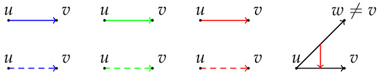
Figure 1.
Illustration of the used notation. Solid blue line: , dashed blue line: , solid green line: , dashed green line: , solid red line: , dashed red line , and red link from to : holds.
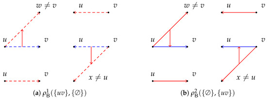
Figure 2.
Counterexamples for including and excluding a single edge .
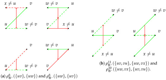
Figure 3.
Counterexamples for including and excluding more than one edge.
Theorem 2.
Let and be two of the vertex preserving simple graph transformations in Γ. Let and be graph classes defined by inclusion, exclusion and transfer predicates satisfying Independence, Transitivity and Soundness (Assumptions 1–3). Let resp. be the expressions listed in Table 4 resp. Table 5 for and . Moreover, let be the maximum size of a minimum witness graph as defined for in Table 3. It holds: if there exists a graph with such that
is satisfied, where and are specific subsets and , as defined in the Table 4 and Table 5 and V is the vertex set of H for each expression.
Proof.
Theorem 1 states that is satisfied if there exists a counter example with a size, at most .
To obtain a graph H such that , but , for the expressions listed in Table 4 resp. Table 5, has to be non-satisfiable, but has to be satisfiable. Hereby, is the graph before considering the graph transformations and means that it is not possible to include all edges in , while excluding all edges in . Consequently, means that it is possible to include all edges in , while excluding all edges in .
The expressions can be derived by the conjunction of the expressions for graph class transformation X in Table 3. For the edges in , the expression for has to be used, while for the edges in the expression for has to be used. The expressions we derive in this way refer to the case that it is possible to include the edges in , while excluding the edges in and therefore yields an expression for . Negating yields the expression for , given in Table 4 resp. Table 5. The expressions for the negated transformations can be obtained by switching the sets and . □
The expression of Theorem 2 simplifies significantly when testing or and if the predicates safisfy two additional properties called predicate-symetric and predicate-forwarding.
Definition 3.
A graph class A is called predicate-symmetric if and holds.
Definition 4.
A graph class A is called predicate-forwarding if and holds.
Obviously, predicate-symmetric and predicate-forwarding graph classes can still satisfy Independence, Transitivity and Soundness (Assumptions 1–3).
The graph classes of the application described in Section 2, are predicate–symmetric and predicate-forwarding.
Corollary 1.
Let be a predicate–symmetric and predicate-forwarding graph class defined by inclusion, exclusion and transfer axioms, satisfying Independency, Transitivity and Soundness (Assumptions 1–3). We have: iff
and iff
is satisfied for some .
Corollary 2.
For predicate–symmetric and predicate-forwarding graph classes Theorem 2 can also be applied for the transformations and by using the following expressions:
Proof.
We have to derive the appropriate expressions for Lemma 4 for this specific case.
If holds, then by the symmetry of the predicates also holds and then and have to be set to . This yields . Analogously, if holds, then by the symmetry of the predicates also holds and then and are both set to , i.e., and holds. This also yields . Since the predicates are furthermore predicate-forwarding, predicates for other edges have no impact on the existence of the edges and . Furthermore, neither nor implies , , , . The only further condition we have to consider is the symmetry of F. Finally, this yields
while no restrictions exist for .
This yields , and = . Due to the symmetry of the transformations, i.e., any edge exists if and only if edge exists, the reaming expressions follow identically by the method applied in Theorem 2. □
5. Example Application
5.1. Manual Application of the Derived Concept
We first illustrate the presented concept manually by applying it to the graph classes discussed in Section 2. We use the concept to demonstrate that the class is the same as class (as already discussed). Moreover, we apply the concept to show that the classes and studied in the literature are in fact classes, with none being contained in the other one.
The inclusion predicate and exclusion predicate are obviously symmetric, as long as is symmetric (which we assume for this example). The class has an inclusion and exclusion but no transfer predicate, i.e., the transfer predicate is always . Thus, for testing and , neither (7) nor (8) of Corollary 1 are satisfied. Thus, both inclusions must be satisfied, and we have in fact the equality of both graph classes.
Now, the relation between and is considered. Applying Corollary 1 together with (i.e., we have only exclusion and transfer predicate) we have to check the satisfiability of
for testing and
for testing .
This yields the counterexample , , , , and , which proves . As well, this yields the counterexample , , , and , which proves . Thus, neither nor is contained in the other class. The according counterexamples can be found in Appendix B with the examples indexed: 52 and 53.
Now let us drop the assumption of the examples in Section 2, that is a metric. Assume that is not required. In this case, the inclusion and exclusion predicate are not necessarily symmetric. Corollary 1 is not applicable. We have to resort to the Theorem 2. The relation between and is now considered again. For testing the relation , the second conjunction of expression (6) yields . Replacing the formula with the predicates by using Table 4 yields .
This formula is satisfied if and or and . Thus, we have found a counter example that the relation does not necessarily hold when is not a metric.
5.2. Automatically Derived Graph Class Relations
The tables in Appendix A show the automatically derived relations between all example geometric graph classes resulting from wireless networks, which we defined in Section 2. Since in this specific case the graph class axioms are predicate-symmetric and predicate-forwarding, we can also check for subclass relations, including the two xor transformations.
In case the relation does not hold, a counter example with at most four vertices can be found. We show the found counter examples in Appendix B. The counter examples are consecutively numbered and labeled with the expression (as defined by Table 4 and Table 5 and the negated forms) which led to unsatisfiability.
The tables in Appendix A are to be read from left to right as follows. Class in row i is related to class in column j according to table entry , by relation:
- =
- The classes are the same
- ⊂
- The class is contained in the other class but the classes are not the same
- ⊃
- The class contains the other class but the classes are not the same
- ×
- Neither of the two classes is contained in the others, (by lemmas 1 and 2 each of the studied graph classes contain at least the null graph. Thus, none of the considered graph classes are disjoint).
The relations ⊂, ⊃ and × in the tables are indexed with the numbered counter examples from Appendix B. Notation refers to the counter example number n, which shows that is not contained in . Analogously, refers to the counter example number n, which shows that is not contained in . Finally, refers to the counter example n, which shows that is not contained in and the counter example m, which shows that is not contained in .
The class name encoding in the tables in Appendix A is as defined at the beginning of the paper, summarized by the following Hasse diagram. To avoid clutter, the tables depict the graph classes without the fixed parameters r and 1.
Class (not defined so far) means all of the predicates (i.e., inclusion, exclusion, and transfer) are . With all preconditions being false, all graphs satisfy inclusion, exclusion, and transfer predicate. Thus, the class just contains all graphs over the given vertex universe .
Classes , and are as already defined based only on inclusion, exclusion, and transfer predicate, respectively. All the remaining classes result from the intersection of the classes, which are predecessors in the diagram (observed from the top to bottom).
The class names and were not used before. We define them here for the sake of the completeness of the tables. For graphs in class (which we term boost graphs), an arbitrary long link can be added to a vertex, which boosts the connectivity of that vertex. It will be connected to all other vertices with the same or less distance. The graphs in class (which we term minimum radius DTGs) are a DTG but also with a minimum connectivity radius, where vertices are always connected.
Opposed to the usual assumption that actually stands for a symmetric subgraph/supergraph of , we denote it here just as to stay consistent with the notation used in the table. Class , as usually used in the literature, can be found under and the same class in the table.
The tables in Appendix A are tiled into blocks, referred to as in the following, each representing the relations of the classes , , , , , , , and under the transformations and , i.e., , and represents the 64 relations given by
All relations in the tables in Appendix A were automatically determined by applying FindInstance of Mathematica 12.1 on the derived expression (6) using the Euclidean metric.
In connection with the relations of the base classes shown in the Hasse diagram in Figure 4, the following observations can be made for the derived tables.
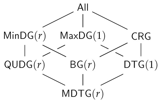
Figure 4.
The relations of the base graph classes.
For each block (i.e. when applying the same transformation to the columns and rows of the block), the row for is the row for but read reversed from right to left instead of left to right. The same applies for the row pairs , , and , (which are not directly connected in the Hasse diagram).
Moreover, the transformations and yield obviously the same graph class when applied on . The same applies to , as already discussed. As well, applied on and as well on , transformations and yield the same classes, respectively.
These base classes (, , and ) are as well exactly those classes whose symmetric variants due to and are contained in the base class. For the other classes neither the subset relation nor superset relation is satisfied between base classes and their symmetric variants.
Both transformations and obviously preserve the subset relation order of the base classes. Moreover, neither nor yield two base classes collapsing into one single class.
The graph class relation for all classes between directed and symmetric, complementry-directed and symmetric, and as well, directed and complementry-directed is always orthogonal, i.e., the block consists only of entries in this case.
Trivially, and consists only of entries =, since the first always yields the empty graph independent of the source graph, while for the latter, it is always the complete graph as well as being independent of the source graph.
Finally, putting all the tables together into one single table (with the same class ordering for rows and columns) yields a trivially symmetric matrix with diagonal entries =, however, with reversed relations ⊂ and ⊃ for all off-diagonal entries.
6. Conclusions
In this paper, we described how to prove or disprove containedness relations of specific axiomatic-described geometric graph classes on a meta-level. We proved the correctness of the general logical existentially quantified expressions over placeholders for inclusion, exclusion, and transitive transfer predicates. We illustrated the concept with concrete predicates in the context of simple theoretical wireless network models.
Though we focused on geometric classes in this work, by its generality, the concept is also applicable to any graph class, which can be described by means of inclusion, exclusion and transfer axioms and simple graph transformations.
The decidability of the problem of testing containedness for concrete inclusion, exclusion and transfer predicates depends on the concrete theories we consider. These are typically extensions of the theory of real numbers with norms, distances, cost functions or more general function symbols. In ongoing work, we are investigating the decidability of such theories.
Though a logical representation of graphs is not new in general, we believe with the axiomatic graph class representation and the discussed simple transformations described in this work, we discovered a promising graph theoretical novel concept for containedness verification, which can be generalized in many further directions.
Future work includes extending the theory beyond simple graph transformations. Moreover, one can drop the condition on transfer predicates to be transitive or even further that the edges involved do not have to be originated at the two vertices to which the transfer predicate is applied.
Author Contributions
L.B. and H.F. contributed equally to this work. All authors have read and agreed to the published version of the manuscript.
Funding
This research received no external funding.
Institutional Review Board Statement
Not applicable.
Informed Consent Statement
Not applicable.
Data Availability Statement
Not applicable.
Acknowledgments
We would like to thank for all discussions with Viorica Sofronie-Stokkermans providing us with background information on the general theory of formal verification.
Conflicts of Interest
The authors declare no conflict of interest.
Appendix A. Automatically Derived Containedness Relations


Appendix B. Automatically Derived Counter Examples


Appendix C. Proof of Lemma 4
Proof.
Two implication directions “⇒” and “⇐” have to be shown.
The proof omitted in the main part is given here in the appendix.
Part 1 (⇒).
With there exists a graph with . The proof is split up in two sub parts. The first part contains the proof that holds for all transformations in and in the second part transformation, specific proofs are considered.
Subpart 1 (all transformations in ).
Subpart 2 (transformation specific part of the proof).
For the identity transformation B holds. With graph class Axiom (3) the expression is derived. Using (A1), (A2) and E(u,w) yields the formula in the table (in the following of this proof, the table always refers to Table 3).
Furthermore, with graph class Axiom (4), the expression is derived. Using (A3), (A4) and yields the formula in the table. Note that the existence of depends only on and for and both formulas in the table yield . Therefore, the expression with the transfer predicate is only written in one of the formulas.
For the transformation, holds. With graph class Axiom (3), the expression is derived. Using (A1), (A2) and yields the formula in the table.
Furthermore, with graph class Axiom (4) the expression is derived. Using (A3), (A4) and yields the formula in the table.
Moreover, for the transformation , the existence of the depends only on one of the edges, in this case . Therefore, it is also enough to write the expression with the transfer predicate in only one of the formulas.
For the transformation and holds. Furthermore, the transformation is symmetric. Therefore, resp. has to be included in the formula.
With graph class Axiom (3), the expression is derived. Using (A1), (A2), and yields the formula in the table.
Furthermore, with graph class Axiom (4) the expression is derived. Using (A3) and (A4) yields the formula in the table. Since the transformation is symmetric, it is enough to list only the condition for in the formula for .
For the , transformation and holds. Furthermore, the transformation is symmetric. Therefore, resp. has to be included in the formula.
With graph class Axiom (3) the expression is derived. Using (A1), (A2) yields the formula in the table. Since the transformation is symmetric, it is enough to list only the condition for in the formula for .
Furthermore, with the graph class Axiom (4), the expression is derived. Using (A3), (A4), and yields the formula in the table.
For the transformation and holds. Furthermore, the transformation is directed. Therefore, holds.
With the graph class Axioms (3) and (4) the expression is derived. Using (A1)–(A4), and yields the formula in the table.
Furthermore, with the graph class Axioms (3) (4), the expression is derived. Using (A1)–(A4), and yields the formula in the table.
For the transformation and holds. Furthermore, the transformation is directed. Therefore, holds.
With the graph class Axioms (3) and (4) the expression is derived. Using (A1)–(A4), and yields the formula in the table.
Furthermore, with the graph class Axioms (3) (4) the expression is derived. Using (A1)–(A4), and yields the formula in the table.
For the transformation no edges can exist, therefore, and hold.
The formulas for the negated transformations can be obtained by switching the formulas for and and also switching and for any pair of vertices inside the formula.
Part 2 (⇐).
Assume now that we have a graph such that the edge inclusion and exclusion implications depicted for in Table 3 are satisfied. We construct a graph such that and , which then implies .
Construction of is conducted in two steps, a preprocessing and a postprocessing step. The preprocessing is the same for all graph class transformations, while for the postprocssing the specific conditions for the graph classes have to be considered. We begin with a configuration, where all are set to . First, we keep those to resp. set those to , which are enforced or forbidden due to the graph class axioms of class . We then set the remaining edges , which have not been determined in preprocessing accordingly, such that G still satisfies and at the same time satisfies .
Preprocessing (forbidden edges): In order to satisfy graph class Axiom (2), for all , which satisfy , we set to ; in this case, in order to also satisfy the Axiom (3), we set to for all for which is satisfied.
Preprocessing (enforced edges): In order to satisfy graph class Axiom (1), for all which satisfy , we set to ; in this case, in order to satisfy also Axiom (3), we set to for all for which is satisfied. Soundness of inclusion, exclusion and transfer predicates assures that we do not set any and to , which we have set to before.
Postprocessing: Now, we consider the implications for the specific transformations.
For the identity transformation B holds; therefore, the edge was not set to in the preprocesing and can be set to now.
Furthermore, assures that was not set to in the preprocessing and is also not enforced by the existence of another edge , since .
For , holds; therefore, the edge was not set to in the preprocessing and can be set to now.
Furthermore, assures that was not set to in the preprocessing and is also not enforced by the existence of another edge , since .
For the transformation we start with the implication for , because and have to be set to for . The implication for assures that was not set to in the prepossessing and is also enforced by the existence of other edges. Therefore, we can set to false now. The symmetry of assures that the same holds for ; therefore, we can also set to false now.
Now, consider the implication for and assume first that holds. This implication assures that was not set to in the preprocessing. Furthermore, can also not be set to , by the non-existence of an other edge, because if holds, then also holds and therefore can be set to , too. Therefore, can be set to now. With the same argument, can be set to if holds.
For the transformation , we start with the implication for , because and have to be set to for . The implication assures that was not set to in the preprocessing and is also not removed by the non-existence of other edges. Therefore, we can set to now.The symmetry of assures that the same holds for ; therefore, we can also set to now.
Now, consider the implication for and assume first that holds. This implication assures that was not set to in the preprocessing. Furthermore, can also not be set to , by the existence of any other edge, because if holds, then also holds and therefore can be set to , too. Therefore, can be set to now. With the same argument can be set to if holds.
For the transformation , we start with the implication for , because has to be set to and has to be set to for . We consider first the first part of the implication that assures that can be set to and afterwards the second part of the implication that assures that can be set to . The implication assures that was not set to in the preprocessing.Furthermore, can also not be set to , by the existence of an other edge, because if holds, then also holds and therefore can be set to as well. Therefore, we can set to now.
The implication assures that was not set to in the prepossessing. Furthermore, can as well not be set to , by the existence of another edge, because if holds, then also holds and therefore can be set to as well. Therefore, we can set to now.
With the same argumentation, the implication for assures that can be set to or can be set to , if holds.
For the transformation , we start with the implication for , because has to be set to and has to be set to for . We consider first the first part of the implication that assures that can be set to and afterwards the second part of the implication that assures that can be set to . The implication assures that was not set to in the preprocessing. Furthermore, can also not be set to , by the existence of an other edge, because if holds, then also holds and therefore can be set to as well. Therefore, we can set to now.
The implication assures that was not set to in the prepossessing. Furthermore, can also be not set to , by the existence of an other edge, because if holds, then also holds and therefore can be set to as well. Therefore, we can set to false now.
With the same argumentation, the implication for assures that can be set to or can be set to if holds.
For the transformation , no transformation specific restrictions have to be considered, because every graph is transformed to the empty graph. Therefore, after the preprocessing, the remaining edges can be set to or arbitrarily.
The proofs for the negated transformations can be obtained analogously. □
References
- Frey, H.; Böltz, L. Automatically Testing Containedness between Geometric Graph Classes defined by Inclusion, Exclusion and Transfer Axioms. In Proceedings of the 33rd Canadian Conference on Computational Geometry, CCCG 2021, Halifax, NS, Canada, 10–12 August 2021; pp. 127–138. [Google Scholar]
- Gabbay, D.M.; Schmidt, R.A.; Szalas, A. Studies in logic: Mathematical logic and foundations. In Second-Order Quantifier Elimination—Foundations, Computational Aspects and Applications; College Publications: Rickmansworth, UK, 2008; Volume 12. [Google Scholar]
- Bachmair, L.; Ganzinger, H.; Waldmann, U. Refutational Theorem Proving for Hierarchic First-Order Theories. Appl. Algebra Eng. Commun. Comput. 1994, 5, 193–212. [Google Scholar] [CrossRef]
- Barrière, L.; Fraigniaud, P.; Narayanan, L.; Opatrny, J. Robust position-based routing in wireless ad hoc networks with irregular transmission ranges. Wirel. Commun. Mob. Comput. 2003, 3, 141–153. [Google Scholar] [CrossRef]
- Kuhn, F.; Wattenhofer, R.; Zollinger, A. Ad hoc networks beyond unit disk graphs. Wirel. Netw. 2008, 14, 715–729. [Google Scholar] [CrossRef]
- Blough, D.M.D.; Leoncini, M.; Resta, G.; Santi, P. The k-Neighbors Approach to Interference Bounded and Symmetric Topology Control in Ad Hoc Networks. IEEE Trans. Mob. Comput. 2006, 5, 1267–1282. [Google Scholar] [CrossRef]
- von Rickenbach, P.; Wattenhofer, R.; Zollinger, A. Algorithmic Models of Interference in Wireless Ad Hoc and Sensor Networks. IEEE/ACM Trans. Netw. 2009, 17, 172–185. [Google Scholar] [CrossRef]
- Peleg, D.; Roditty, L. Localized spanner construction for Ad Hoc networks with variable transmission range. ACM Trans. Sens. Netw. 2010, 7, 25:1–25:14. [Google Scholar] [CrossRef]
- Moaveninejad, K.; Song, W.Z.; Li, X.Y. Robust position-based routing for wireless ad hoc networks. Ad Hoc Netw. 2005, 3, 546–559. [Google Scholar] [CrossRef]
Publisher’s Note: MDPI stays neutral with regard to jurisdictional claims in published maps and institutional affiliations. |
© 2022 by the authors. Licensee MDPI, Basel, Switzerland. This article is an open access article distributed under the terms and conditions of the Creative Commons Attribution (CC BY) license (https://creativecommons.org/licenses/by/4.0/).