SWAR: A Deep Multi-Model Ensemble Forecast Method with Spatial Grid and 2-D Time Structure Adaptability for Sea Level Pressure

Abstract
1. Introduction
2. Related Work
3. Method
3.1. Window Self-Attention
3.2. Shifted Window Attention
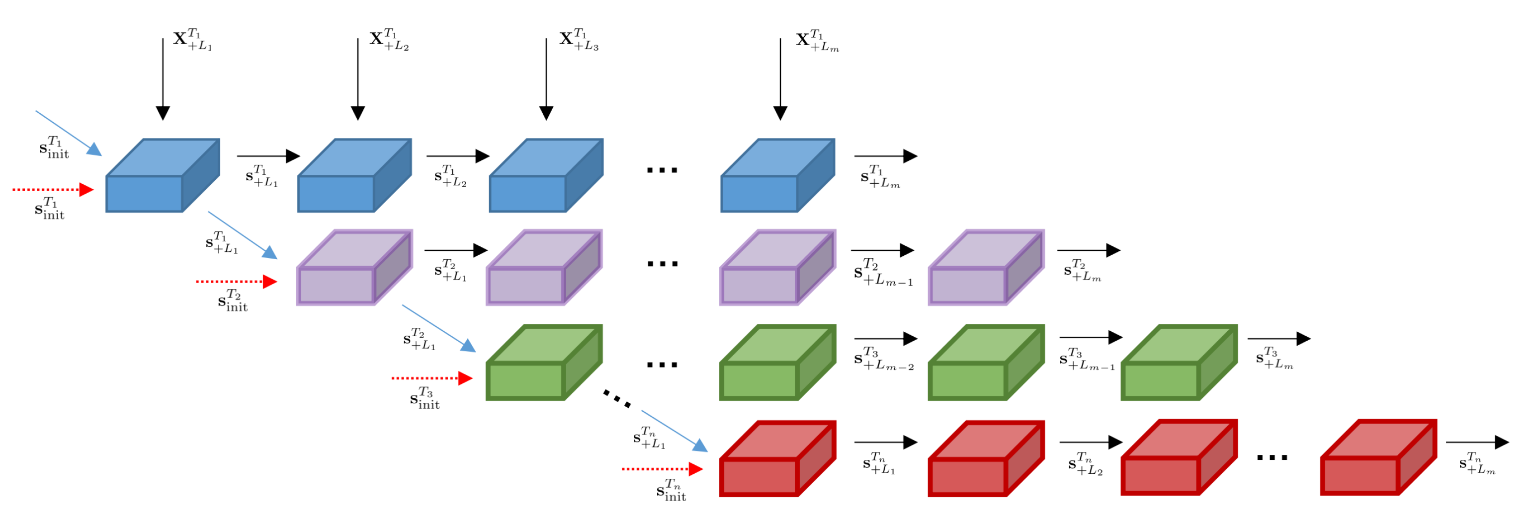
3.3. Roll-RLNN for 2D Time Structure
3.4. Model Structure
4. Experiment
4.1. Data Selection
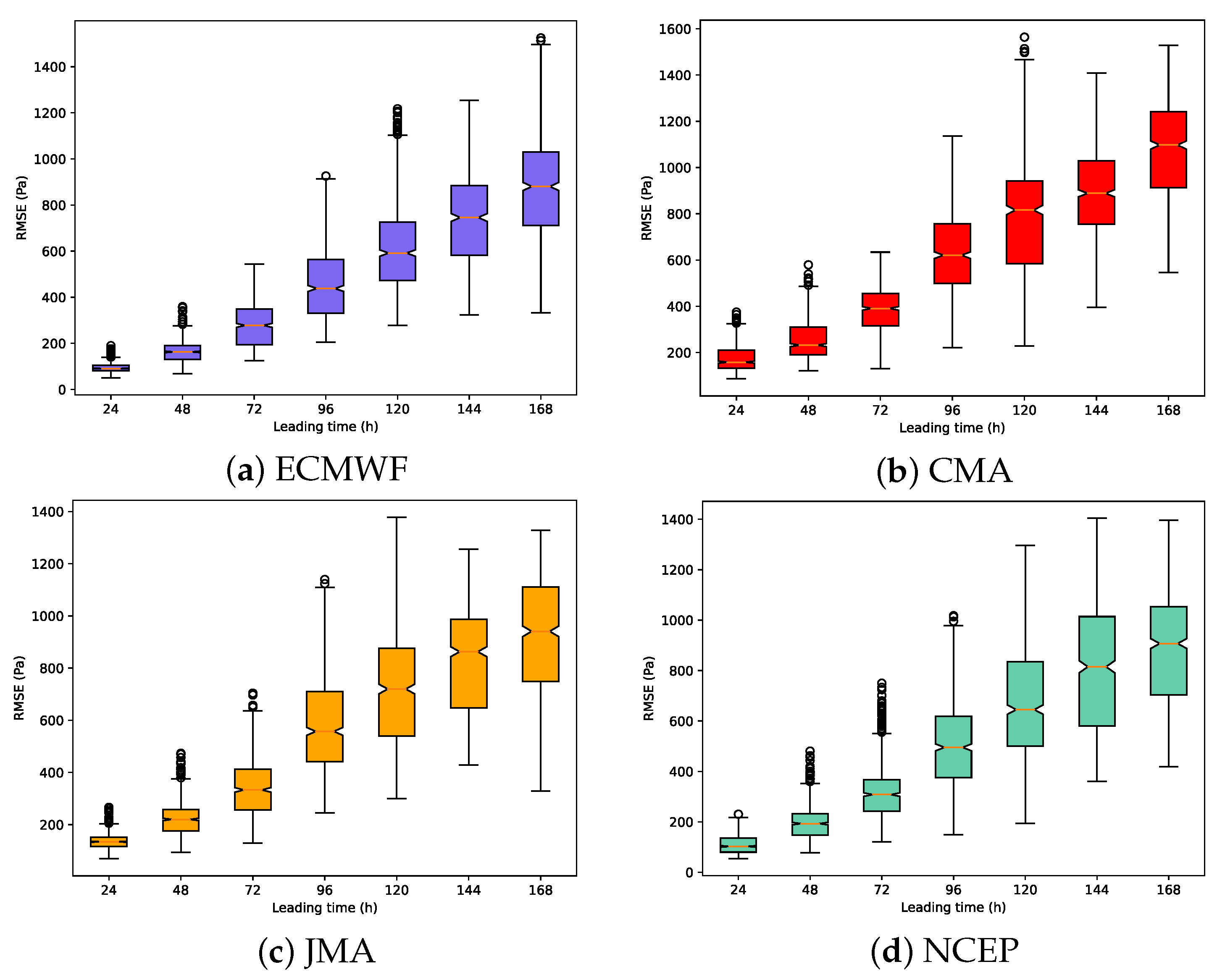
4.2. Data Analysis
4.3. Metrics
4.4. Model Selection and Main Hyper-Parameters
4.5. Result and Analysis
4.6. Discussion
5. Conclusions
Author Contributions
Funding
Data Availability Statement
Conflicts of Interest
Appendix A


References
- Zhu, Y. Ensemble forecast: A new approach to uncertainty and predictability. Adv. Atmos. Sci. 2005, 22, 781–788. [Google Scholar] [CrossRef]
- Zhang, H.; Pu, Z. Beating the Uncertainties: Ensemble Forecasting and Ensemble-Based Data Assimilation in Modern Numerical Weather Prediction. Adv. Meteorol. 2010, 2010, 432160. [Google Scholar] [CrossRef]
- Doblas-reyes, F.J.; Hagedorn, R.; Palmer, T.N. The rationale behind the success of multi-model ensembles in seasonal forecasting—II. Calibration and combination. Tellus Ser. A-Dyn. Meteorol. Oceanol. 2005, 57, 234–252. [Google Scholar]
- Weigel, A.P.; Liniger, M.A.; Appenzeller, C. Can multi-model combination really enhance the prediction skill of probabilistic ensemble forecasts? Q. J. R. Meteorol. Soc. 2008, 134, 241–260. [Google Scholar] [CrossRef]
- Deconinck, W. Development of Atlas, a flexible data structure framework. arXiv 2019, arXiv:1908.06091. [Google Scholar]
- Krishnamurti, T.N.; Kumar, V.; Simon, A.; Bhardwaj, A.; Ghosh, T.; Ross, R. A review of multimodel superensemble forecasting for weather, seasonal climate, and hurricanes. Rev. Geophys. 2016, 54, 336–377. [Google Scholar] [CrossRef]
- Zhi, X.; Qi, H.; Bai, Y.; Lin, C. A comparison of three kinds of multimodel ensemble forecast techniques based on the TIGGE data. Acta Meteorol. Sin. 2012, 26, 41–51. [Google Scholar] [CrossRef]
- Taillardat, M.; Mestre, O.; Zamo, M.; Naveau, P. Calibrated Ensemble Forecasts Using Quantile Regression Forests and Ensemble Model Output Statistics. Mon. Weather Rev. 2016, 144, 2375–2393. [Google Scholar] [CrossRef]
- Yang, T.; Hao, X.; Shao, Q.; Xu, C.-Y.; Zhao, C.; Chen, X.; Wang, W. Multi-model ensemble projections in temperature and precipitation extremes of the Tibetan Plateau in the 21st century. Glob. Planet Chang. 2012, 80–81, 1–13. [Google Scholar] [CrossRef]
- Wang, K.; Zheng, X.; Wang, G.; Liu, D.; Cui, N. A Multi-Model Ensemble Approach for Gold Mineral Prospectivity Mapping: A Case Study on the Beishan Region, Western China. Minerals 2020, 126, 1126. [Google Scholar] [CrossRef]
- Raghavendra, S.; Deka, P.C. Support vector machine applications in the field of hydrology: A review. Appl. Soft Comput. J. 2014, 19, 372–386. [Google Scholar] [CrossRef]
- Abuella, M.; Chowdhury, B. Random forest ensemble of support vector regression models for solar power forecasting. In Proceedings of the 2017 IEEE Power & Energy Society Innovative Smart Grid Technologies Conference (ISGT), Washington, DC, USA, 23–26 April 2017; pp. 1–5. [Google Scholar]
- Wang, B.; Zheng, L.; Liu, D.L.; Ji, F.; Clark, A.; Yu, Q. Using multi-model ensembles of CMIP5 global climate models to reproduce observed monthly rainfall and temperature with machine learning methods in Australia. Int. J. Climatol. 2018, 38, 4891–4902. [Google Scholar] [CrossRef]
- Tao, Y.; Yang, T.; Faridzad, M.; Jiang, L.; He, X.; Zhang, X. Non-stationary bias correction of monthly CMIP5 temperature projections over China using a residual-based bagging tree model. Int. J. Climatol. 2018, 38, 467–482. [Google Scholar] [CrossRef]
- Scher, S. Toward Data-Driven Weather and Climate Forecasting: Approximating a Simple General Circulation Model With Deep Learning. Geophys. Res. Lett. 2018, 45, 12616–12622. [Google Scholar] [CrossRef]
- Kumar, A.; Mitra, A.K.; Bohra, A.K.; Iyengar, G.R.; Durai, V.R. Multi-model ensemble (MME) prediction of rainfall using neural networks during monsoon season in India. Mereorol. Appl. 2012, 19, 161–169. [Google Scholar] [CrossRef]
- Kim, J.; Kim, K.; Cho, J.; Kang, Y.Q.; Yoon, H.-J.; Lee, Y.-W. Satellite-Based Prediction of Arctic Sea Ice Concentration Using a Deep Neural Network with Multi-Model Ensemble. Remote Sens. 2019, 11, 19. [Google Scholar] [CrossRef]
- Li, D.; Marshall, L.; Liang, Z.; Sharma, A. Hydrologic multi-model ensemble predictions using variational Bayesian deep learning. J. Hydrol. 2022, 604, 127221. [Google Scholar] [CrossRef]
- Grönquist, P.; Yao, C.; Ben-Nun, T.; Dryden, N.; Dueben, P.; Li, S.; Hoefler, T. Deep learning for post-processing ensemble weather forecasts. Philos. Trans. R. Soc. A 2021, 379, 20200092. [Google Scholar] [CrossRef]
- Hu, Y.-F.; Yin, F.-K.; Zhang, W.-M. Deep learning-based precipitation bias correction approach for Yin–He global spectral model. Mereorol. Appl. 2021, 28, e2032. [Google Scholar] [CrossRef]
- Wang, X.; He, X.; Cao, Y.; Liu, M.; Chua, T.-S. KGAT: Knowledge Graph Attention Network for Recommendation. In Proceedings of the 25th ACM SIGKDD International Conference on Knowledge Discovery & Data Mining, Anchorage, AK, USA, 4–8 August 2019; pp. 950–958. [Google Scholar]
- Qin, Y.; Song, D.; Cheng, H.; Cheng, W.; Jiang, G.; Cottrell, G.W. A Dual-Stage Attention-Based Recurrent Neural Network for Time Series Prediction. In Proceedings of the 26th International Joint Conference on Artificial Intelligence, Melbourne, VIC, Australia, 19–25 August 2017; pp. 2627–2633. [Google Scholar]
- Trebing, K.; Staundefinedczyk, T.; Mehrkanoon, S. SmaAt-UNet: Precipitation Nowcasting Using a Small Attention-UNet Architecture. Pattern Recogn. Lett. 2021, 145, 178–186. [Google Scholar] [CrossRef]
- Sperber, M.; Niehues, J.; Neubig, G.; Stüker, S.; Waibel, A. Self-Attentional Acoustic Models. arXiv 2018, arXiv:1803.09519. [Google Scholar]
- Li, X.; Zhong, Z.; Wu, J.; Yang, Y.; Lin, Z.; Liu, H. Expectation-Maximization Attention Networks for Semantic Segmentation. In Proceedings of the 2019 IEEE/CVF International Conference on Computer Vision (ICCV), Anchorage, AK, USA, 4–8 August 2019; pp. 9166–9175. [Google Scholar]
- Sinha, A.; Dolz, J. Multi-Scale Self-Guided Attention for Medical Image Segmentation. IEEE J. Biomed. Health Inform. 2021, 25, 121–130. [Google Scholar] [CrossRef]
- Beltagy, I.; Fischer, P.; Peters, M.E.; Cohan, A. Longformer: The Long-Document Transformer. arXiv 2020, arXiv:2004.05150. [Google Scholar]
- Huang, T.; Deng, Z.-H.; Shen, G.; Chen, X. A Window-Based Self-Attention approach for sentence encoding. Neurocomputing 2020, 375, 25–31. [Google Scholar] [CrossRef]
- Liu, Z.; Lin, Y.; Cao, Y.; Hu, H.; Wei, Y.; Zhang, Z.; Lin, S.; Guo, B. Swin Transformer: Hierarchical Vision Transformer using Shifted Windows. In Proceedings of the 2021 IEEE/CVF International Conference on Computer Vision (ICCV), Seoul, Republic of Korea, 27 October–2 November 2019; pp. 9992–10002. [Google Scholar]
- Jankov, I.; Toth, Z.; Feng, J. Initial-Value vs. Model-Induced Forecast Error: A New Perspective. Meteorology 2022, 1, 377–393. [Google Scholar] [CrossRef]
- ECMWF. Public Datasets. Available online: https://apps.ecmwf.int/datasets/ (accessed on 3 November 2022).
- Shi, X.; Chen, Z.; Wang, H.; Yeung, D.-Y.; Wong, W.; Woo, W. Convolutional LSTM Network: A Machine Learning Approach for Precipitation Nowcasting. In Proceedings of the 28th International Conference on Neural Information Processing Systems (NIPS), Montreal, QC, Canada, 7–12 December 2015; Volume 1, pp. 802–810. [Google Scholar]
- Ronneberger, O.; Fischer, P.; Brox, T. U-Net: Convolutional Networks for Biomedical Image Segmentation. arXiv 2015, arXiv:1505.04597. [Google Scholar]


| Model | +24 h | +48 h | +72 h | +96 h | ||||||||
|---|---|---|---|---|---|---|---|---|---|---|---|---|
| RMSE | MAE | PCC | RMSE | MAE | PCC | RMSE | MAE | PCC | RMSE | MAE | PCC | |
| DT | 126.208 | 87.368 | 0.994 | 185.501 | 125.377 | 0.986 | 300.418 | 201.574 | 0.967 | 503.602 | 318.338 | 0.921 |
| GB | 102.731 | 67.270 | 0.996 | 171.424 | 112.343 | 0.988 | 292.453 | 192.398 | 0.969 | 504.759 | 312.386 | 0.919 |
| RF | 94.315 | 63.805 | 0.996 | 167.639 | 110.257 | 0.988 | 292.668 | 192.152 | 0.969 | 503.383 | 311.972 | 0.920 |
| XGB | 92.626 | 67.679 | 0.996 | 163.535 | 109.848 | 0.989 | 283.470 | 187.868 | 0.968 | 469.173 | 293.680 | 0.925 |
| SWA-CL | 89.083 | 65.325 | 0.996 | 151.797 | 105.002 | 0.989 | 264.170 | 178.169 | 0.970 | 445.296 | 282.896 | 0.929 |
| Roll-CL | 91.566 | 67.233 | 0.996 | 153.388 | 106.187 | 0.989 | 262.310 | 176.907 | 0.971 | 440.072 | 280.781 | 0.931 |
| CL | 95.930 | 67.968 | 0.997 | 159.746 | 112.429 | 0.989 | 268.090 | 184.177 | 0.970 | 447.983 | 289.133 | 0.930 |
| UNet | 98.481 | 72.873 | 0.996 | 164.132 | 117.063 | 0.989 | 277.783 | 191.349 | 0.970 | 454.062 | 294.262 | 0.929 |
| SWAR | 83.609 | 59.915 | 0.997 | 150.605 | 103.875 | 0.990 | 261.938 | 176.478 | 0.971 | 439.511 | 279.317 | 0.932 |
| Model | +120 h | +144 h | +168 h | 24–168 h Total | |||||||
|---|---|---|---|---|---|---|---|---|---|---|---|
| RMSE | MAE | PCC | RMSE | MAE | PCC | RMSE | MAE | PCC | RMSE | MAE | |
| DT | 642.046 | 430.539 | 0.867 | 717.626 | 517.745 | 0.826 | 783.186 | 590.553 | 0.781 | 525.737 | 324.499 |
| GB | 638.788 | 427.813 | 0.867 | 706.723 | 511.629 | 0.828 | 786.386 | 592.114 | 0.779 | 521.832 | 316.565 |
| RF | 644.399 | 429.011 | 0.866 | 711.593 | 516.490 | 0.826 | 789.610 | 594.304 | 0.776 | 523.879 | 316.856 |
| XGB | 594.146 | 392.576 | 0.885 | 658.684 | 473.069 | 0.854 | 738.228 | 552.677 | 0.808 | 488.095 | 296.771 |
| SWA-CL | 563.566 | 375.682 | 0.889 | 626.763 | 454.223 | 0.861 | 709.431 | 531.911 | 0.822 | 464.878 | 284.744 |
| Roll-CL | 561.720 | 373.089 | 0.889 | 631.069 | 454.889 | 0.860 | 714.089 | 534.695 | 0.821 | 465.692 | 284.826 |
| CL | 567.243 | 377.326 | 0.888 | 631.731 | 454.207 | 0.860 | 720.928 | 535.804 | 0.820 | 470.238 | 288.721 |
| UNet | 576.224 | 382.694 | 0.887 | 633.582 | 455.086 | 0.860 | 706.553 | 530.050 | 0.823 | 470.964 | 291.911 |
| SWAR | 562.694 | 371.838 | 0.889 | 628.396 | 451.946 | 0.861 | 711.579 | 531.609 | 0.821 | 464.344 | 282.140 |
Publisher’s Note: MDPI stays neutral with regard to jurisdictional claims in published maps and institutional affiliations. |
© 2022 by the authors. Licensee MDPI, Basel, Switzerland. This article is an open access article distributed under the terms and conditions of the Creative Commons Attribution (CC BY) license (https://creativecommons.org/licenses/by/4.0/).
Share and Cite
Zhang, J.; Xu, L.; Jin, B. SWAR: A Deep Multi-Model Ensemble Forecast Method with Spatial Grid and 2-D Time Structure Adaptability for Sea Level Pressure. Information 2022, 13, 577. https://doi.org/10.3390/info13120577
Zhang J, Xu L, Jin B. SWAR: A Deep Multi-Model Ensemble Forecast Method with Spatial Grid and 2-D Time Structure Adaptability for Sea Level Pressure. Information. 2022; 13(12):577. https://doi.org/10.3390/info13120577
Chicago/Turabian StyleZhang, Jingyun, Lingyu Xu, and Baogang Jin. 2022. "SWAR: A Deep Multi-Model Ensemble Forecast Method with Spatial Grid and 2-D Time Structure Adaptability for Sea Level Pressure" Information 13, no. 12: 577. https://doi.org/10.3390/info13120577
APA StyleZhang, J., Xu, L., & Jin, B. (2022). SWAR: A Deep Multi-Model Ensemble Forecast Method with Spatial Grid and 2-D Time Structure Adaptability for Sea Level Pressure. Information, 13(12), 577. https://doi.org/10.3390/info13120577