Abstract
An adaptive optics scanning laser ophthalmoscope (AOSLO) has the characteristics of a high resolution and a small field of view (FOV), which are greatly affected by eye motion. Continual eye motion will cause distortions both within the frame (intra-frame) and between frames (inter-frame). Overcoming eye motion and achieving image stabilization is the first step and is of great importance in image analysis. Although cross-correlation-based methods enable image registration to be achieved, the manual identification and distinguishing of images with saccades is required; manual registration has a high accuracy, but it is time-consuming and complicated. Some imaging systems are able to compensate for eye motion during the imaging process, but special hardware devices need to be integrated into the system. In this paper, we proposed a deep-learning-based algorithm for automatic image stabilization. The algorithm used the VGG-16 network to extract convolution features and a correlation filter to detect the position of reference in the next frame, and finally, it compensated for displacement to achieve registration. According to the results, the mean difference in the vertical and horizontal displacement between the algorithm and manual registration was 0.07 pixels and 0.16 pixels, respectively, with a 95% confidence interval of (−3.26 px, 3.40 px) and (−4.99 px, 5.30 px). The Pearson correlation coefficients for the vertical and horizontal displacements between these two methods were 0.99 and 0.99, respectively. Compared with cross-correlation-based methods, the algorithm had a higher accuracy, automatically removed images with blinks, and corrected images with saccades. Compared with manual registration, the algorithm enabled manual registration accuracy to be achieved without manual intervention.
1. Introduction
Observing retinal structures in high-resolution images is a crucial step in the further investigation of retinal physiology and pathology. A number of imaging modalities are currently employed in the research and diagnostics of ophthalmic conditions, including fundus cameras [1,2], optical coherence tomography (OCT) [3,4,5,6,7], scanning laser ophthalmoscopes (SLOs) [8,9,10,11,12], and adaptive optics scanning laser ophthalmoscopes (AOSLOs) [13,14,15,16].
An AOSLO provides the possibility of observing the structure and activity of the retina at the cellular level. The AOSLO technique has been used increasingly over the past 21 years to study aspects of the retina, such as understanding neonatal neural circuits in the retina [17], monitoring blood flow [18], and analyzing the flux and velocity of retinal capillary erythrocytes [19].
An AOSLO’s high-resolution imaging, however, has the characteristics of a high resolution and a small field of view (FOV), which are greatly affected by involuntary eye motion. Human eyes are constantly moving with a bandwidth of ~100 Hz. If the image acquisition speed is not sufficient or if real-time tracking mechanisms are not implemented in the imaging system, continual retinal motion will cause distortions both within the frame (intra-frame) and between frames (inter-frame) [20], reducing the visibility of retinal structures in the images and resulting in difficulties in the image analysis. Consequently, before performing an image analysis, the sequence of the AOSLO images needs to be stabilized to a common reference to reduce the effects of eye motion.
At present, the common method of stabilizing images is cross-correlation (or Fourier transform)-based methods [20,21,22], which involve time-consuming manual registration. Although cross-correlation methods can successfully identify and differentiate the segments of images with slow drifts, the images with saccades must be identified and differentiated manually. In addition, in order to ensure complete imaging, the imaging system constantly changes the imaging position during the imaging process. In order to adapt to the changes in the imaging position, the cross-correlation methods need to manually change the reference. In addition to postprocessing methods, some imaging systems [23,24,25,26,27,28,29] are capable of compensating for movement during the imaging process, but special hardware equipment with corresponding optics needs to be integrated into the imaging system.
Deep learning has been widely used in computer vision and medical image processing [30,31]. Deep convolutional features have large perceptual fields and rich semantic information, which are suitable for target detection and localization. Therefore, to solve the problems we described above, this paper proposed an automatic algorithm based on the VGG-16 network [32] and a correlation filter [33]. The VGG-16 network was used to extract features, and the correlation filter was used to detect the position of the reference in the next frame and obtain the displacement.
The contributions of this article are as follows: An automatic algorithm was proposed to remove images with blinks and correct images with saccades. To overcome the reference lost due to eye motion or changes in the imaging position, we proposed the method of resetting the training set. This method resets the sample weights and enables the subsequent sample weight to be correctly updated.
2. Materials and Methods
2.1. Data
We acquired 6 videos (2507 frames in total and a frame rate of 30 frames per second (fps)) using a bimorph deformable mirror-based AOSLO (Jiangsu Key Laboratory of Medical Optics, Suzhou Institute of Biomedical Engineering and Technology, Chinese Academy of Sciences) from subjects with normal eye health; for details, see [34]. These videos had 2507 frames in total, of which 201 were frames with blinks. The frame size was 512 × 449 pixels and the field of view (FOV) was 1.5° on the human retina. A transverse region of 445 × 445 µm was scanned using an effective focal length of 17 mm for the eye.
2.2. Baseline Approach ECO: Efficient Convolution Operators for Tracking
For the readers’ convenience, the efficient convolution operators for tracking (ECO) algorithm [35] is summarized here. The ECO core step diagram is shown in Figure 1. ECO extracts the VGGNet features, a histogram of oriented gradient (HOG) features, and color name (CN) features for training the correlation filters to achieve their target localization. A correlation filter was used to describe the similarity between two images. The response values were in the range of 0 to 1, and a higher response value indicated a higher similarity between the target region and the region to be detected.

Figure 1.
Efficient convolution operators for tracking (ECO) core step diagram. Here is an example of the first two frames of the sequence. The scale bar is 100 µm. The green and red boxes are the ECO reference.
ECO trained the parameters of the correlation filter by extracting the features of the samples. The sample was the whole image (as shown in Figure 1). ECO used an interpolation algorithm for the feature of the samples (see Equation (1)).
Here, denotes the d-channel feature (); is a function of , the result of the interpolation of ; is a function of ; is the resolution; is the d-channel feature interpolation function; and we used to denote the entire interpolated feature map, where . Then, ECO used principal component analysis (PCA) to simplify the filter and convolve with to calculate the response value (see Equation (2)).
Here, is the filter; is the convolution operator; and is the projection matrix of rows and columns. Based on the maximum correlation response value (abbreviated as the response value), the predicted position of the reference in the next frame was obtained. The displacement was the difference between the predicted position of the reference and the position in the first frame. Finally, ECO took the norm of the difference between and the labeled detection scores , and added a penalty term to construct the loss function (see Equation (3)).
Here, and are the mean and sample weights, respectively; is the total number of samples; and is the penalty term for . The sample weights controlled the impact of each sample. In addition, we included a spatial regularization term determined by the penalty term . By controlling the spatial extent of the filter , the regularization enabled the filter to be learned on arbitrarily large image regions. The spatial region corresponding to the background features was assigned a large penalty in , while the target region had a small penalty value.
2.3. Our Approach
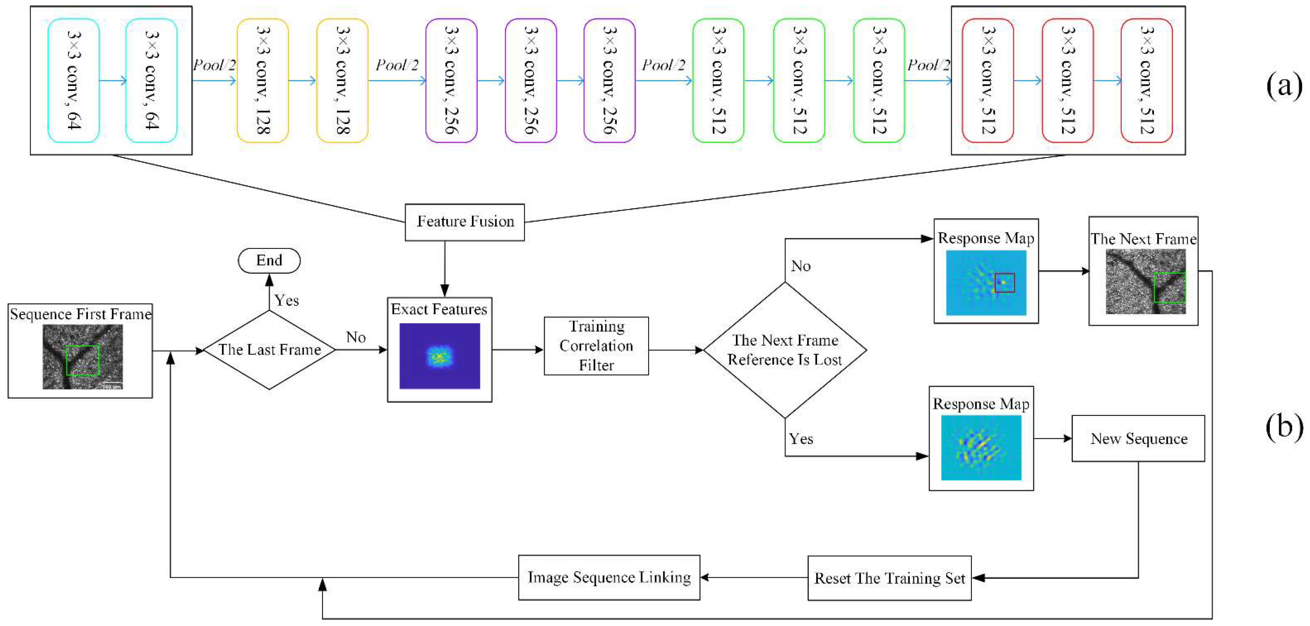
In most of the cases, the reference was lost or partially lost in the AOSLO images due to eye motion and imaging position changes. Although ECO is capable of extracting features from the AOSLO retinal images, it is not capable of handling this particular situation. Thus, we proposed an image stabilization algorithm for AOSLO images called the update efficient convolution operators for imaging stabilization (UECO). Its core step diagram is shown in Figure 2. UECO is divided into two processes: feature extraction and localization, which correspond to VGG-16 and the correlation filter, respectively. The VGG-16 network, from [36], was pre-trained on ImageNet [37]. The pre-trained VGG-16 network was used to extract convolutional features, and the correlation filter was used to detect the position of the reference in the next frame and obtain the displacement.
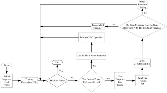
Figure 2.
Update efficient convolution operators for imaging stabilization (UECO) flowchart. UECO trains the initial correlation filter with the initial image sequence. When the reference is lost, UECO resets the training set and starts a new process, taking the current frame as the first frame of the sequence. Finally, by image sequence linking, UECO links image sequences with the same reference together.
We did not need to train the VGG-16 again. Firstly, VGG-16 has a 16-layer network structure, and the last three layers are used for classification. We only needed to extract image features without classification. Secondly, the pre-trained VGG-16 has good generalization. VGG-16 has a deep network structure and can extract the features of any image. VGG-16 is able to extract shallow features (conv3-64) and deep features (conv3-512). The channels and dimensions of the feature vector are merged by the cascade, and then the fused features are obtained by nonlinear mapping through the convolution layer (see Figure 3). In addition, ECO performs well in target tracking using these two convolution features and has demonstrated outstanding results on four tracking benchmarks: VOT2016 [38], UAV123 [39], OTB-2015 [40], and Temple-Color [41].
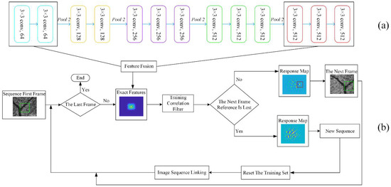
Figure 3.
VGG-16 network structure diagram and UECO core step diagram; (a) is the 5 convolution groups of VGG-16, and the convolution groups are connected by a pooling layer. (b) is the UECO core diagram. The kernel size of the convolution layer in the convolution group was 3 3, and the number of channels in each convolution group was 64, 128, 256, and 512, respectively. The window size of the pooling layer was 2 2, reducing the feature map to 1/2 of its original size. The features of the first convolution group (conv3-64) and the features of the fifth convolution group (conv3-512) were fused by a cascade to train the correlation filter. The scale bar is 100 µm. The green and red boxes in (b) are the UECO reference.
Due to eye motion, the reference had a wide range of displacement, so the central region of the first frame in the sequence was set as the reference, and the relative displacement of the reference was assumed to be 0. The reference size was 200 × 200 pixels. Once the reference was lost, the UECO reset the training set (the details are described in the section on resetting the training set) and selected the central region of the current frame as the new reference, ensuring that the new process was not affected by the correlation filter parameters trained with the samples from the previous process. Finally, through image sequence linking (the details are described in the section on image sequence linking), UECO linked the image sequences with the same reference together.
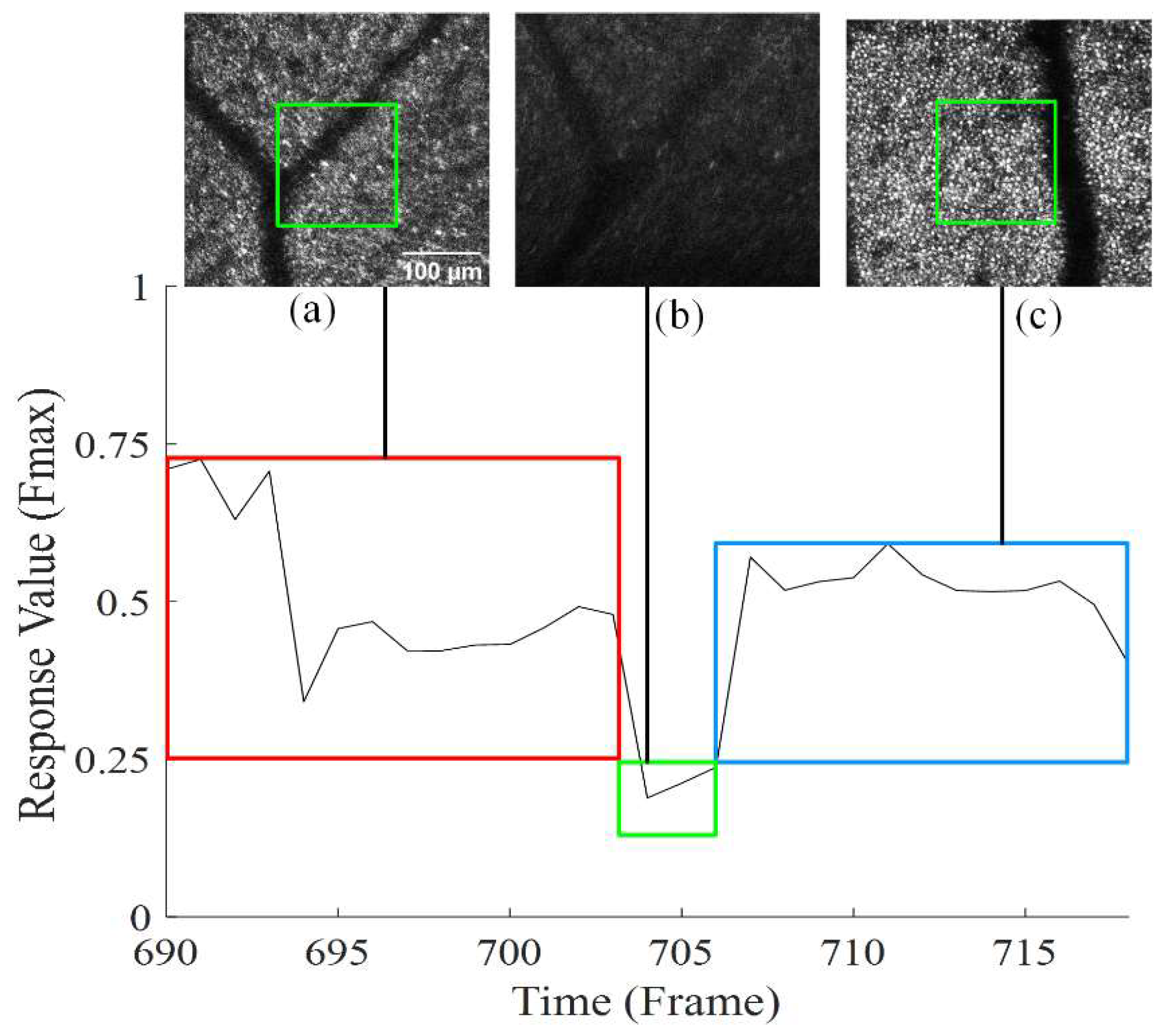
UECO may determine whether a reference is lost based on the and make modifications accordingly. In general, the closer the predicted reference is to the correct reference, the greater the positioning accuracy and the greater the response value. We tested 6 videos with a total of 2507 frames, of which 201 were frames with blinks. The results showed that when the selected reference was accurately predicted, the average was about 0.5. A threshold of 0.25 (half of the average response value) can be used effectively to determine whether the reference has been lost.
As shown in Figure 4, when the selected reference was accurately predicted, was generally around 0.5. In the green boxes, the reference was lost due to intra-frame distortion, and the response values of these frames were all less than the threshold value. After the reference was reselected, rose.
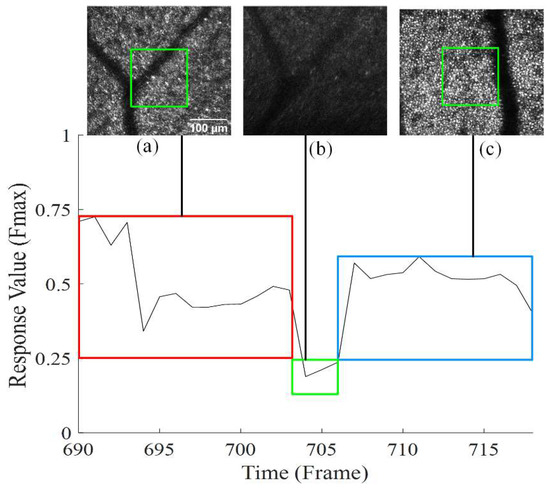
Figure 4.
The response value ; (a,c) are the references of the two sequences (the red and blue boxes represent that the reference is not lost, 0.25) and (b) indicates the reference lost (the green box represents that the reference is lost, 0.25). The scale bar is 100 µm. The green boxes in (a,c) are the UECO reference.
2.3.1. Preprocessing
Preprocessing is used to remove images with blinks. During the imaging process, blinking by the subjects will block the imaging light, and after binarization, the whole image turns black. The Otsu algorithm [42] is an efficient algorithm for binarizing images, which is not affected by image brightness and contrast. In the preprocessing, Otsu is used to binarizes the images, set the threshold to 0, and remove the images with blinks (the all-black images). Partial-blink images can still be mapped to the reference image. Whether the partial-blink image is useful is left for the user to judge.
2.3.2. Reset Training Set
ECO is used in the field of object tracking in computer vision. It is set to track a fixed reference, so the reference does not change. However, the reference of the AOSLO retinal images is often lost due to changes in the imaging position or eye motion. When the reference is lost (current frame response value is lower than 0.25), it needs to be replaced with a new reference, and the samples in the training set are called old samples. As long as the training set is not reset, the training set will always contain old samples, and the correlation filter parameters will always be affected by the old samples and will not be updated correctly, reducing the accuracy of reference localization.
We proposed a solution to this problem by resetting the training set after the reference was lost, selecting the center region of the current frame as the new reference, and retraining the correlation filter parameters with the new samples. UECO reset the training set sample weights; initialized the sample weights , and as the algorithm ran, the sample weights , where the learning rate is (the learning rate inherited from ECO); and normalized the weights .
2.3.3. Image Sequence Linking
The image may return to its original position following a brief blink or eye motion. Therefore, it is necessary to link image sequences with the same reference together. UECO saves the parameters of the correlation filter when using each image sequence to train, and uses the correlation filter to detect each image in sequence. A response value of 0.25 indicates that the two sequences have the same reference and should be linked, otherwise they are independent.
3. Results
The test video had 1163 frames in total, and 1017 frames after preprocessing. Manual registration was performed by two trained medical students and resulted in the removal of 159 distorted images, which was verified by a clinical ophthalmologist with more than five years of experience.
3.1. Experimental Environment
The operating system used in this experiment was Windows 10, the CPU was a 2.9 GHz 8-core AMD Ryzen 7 4800H, the GPU was NVIDIA GeForce RTX 2060, and the memory was 16 GB.
3.2. Comparison with Manual Registration
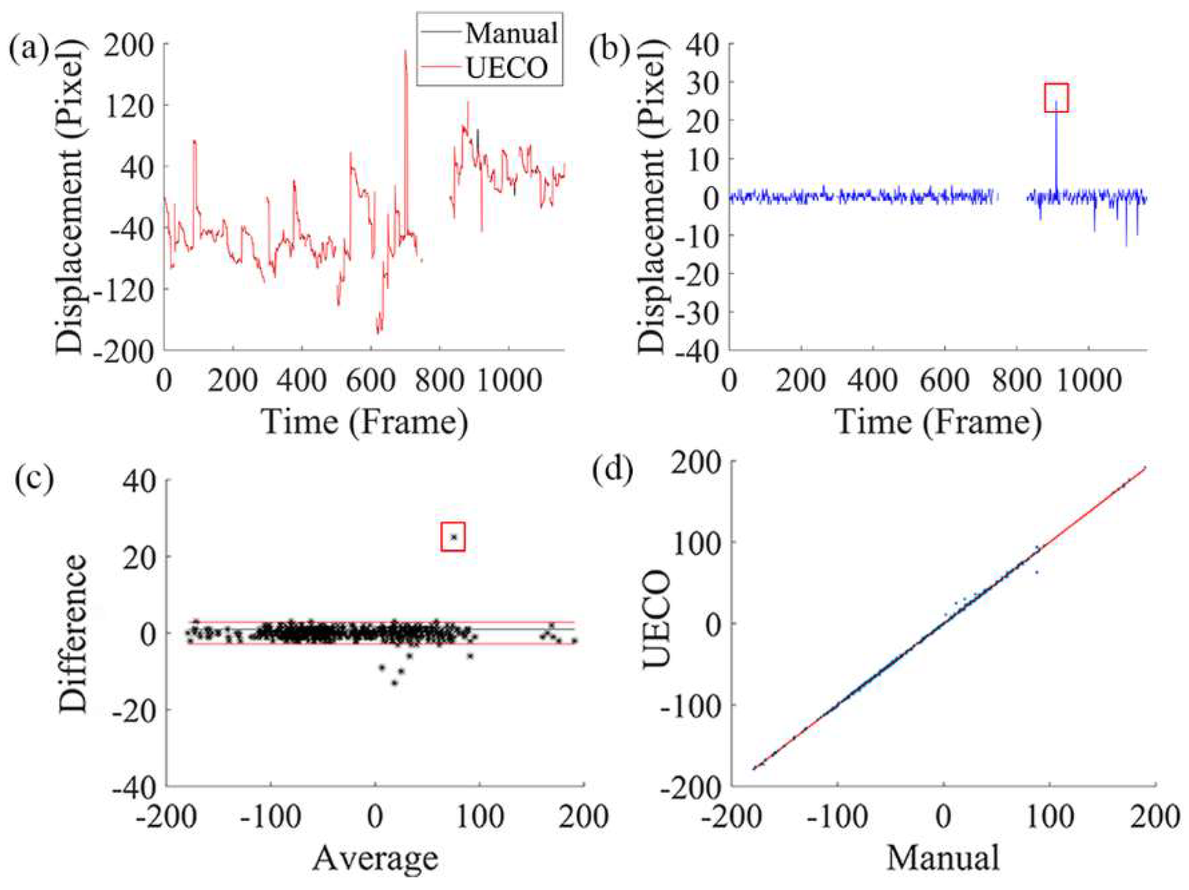
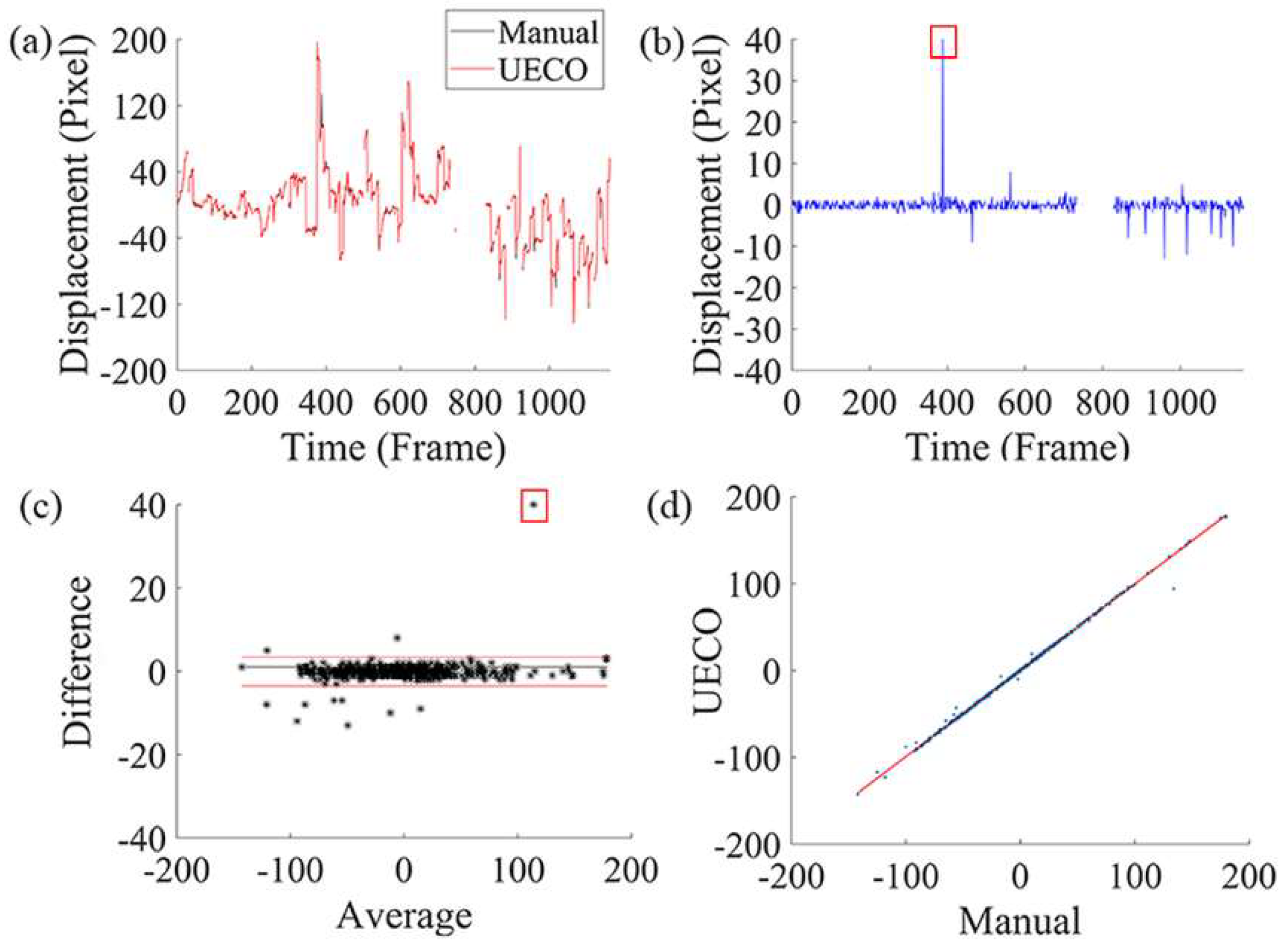
Figure 5 and Figure 6 show the comparison of the displacement obtained by UECO and manual registration. The mean difference in the vertical and horizontal displacement between UECO and manual registration was 0.07 pixels and 0.16 pixels, respectively, with a 95% confidence interval of (−3.26 px, 3.40 px) and (−4.99 px, 5.30 px). The Pearson correlation coefficients were 0.99 and 0.99, respectively.
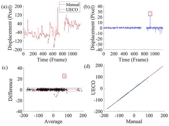
Figure 5.
Vertical displacement comparison chart; (a) shows the comparison of the vertical displacements obtained by UECO and manual registration; (b) is the difference between the two methods; and (c) is the Bland−Altman plot. The black line is the mean difference of the two methods. Red lines indicate the 95% confidence interval (mean 1.96 standard deviation). The Pearson correlation coefficient curve is shown in (d). The frames with the largest differences have been marked with red boxes. The frame number in the x-axis corresponds to the frame number in the original video.
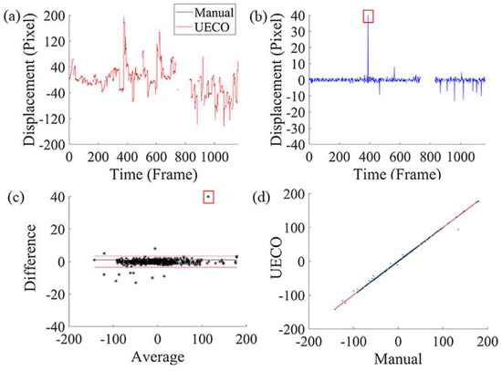
Figure 6.
Horizontal displacement comparison chart; (a) shows the comparison of the horizontal displacements obtained by UECO and manual registration; (b) is the difference between the two methods; and (c) is the Bland−Altman plot. The black line is the mean difference of the two methods. Red lines indicate the 95% confidence interval (mean 1.96 standard deviation). The Pearson correlation coefficient curve is shown in (d). The frames with the largest differences have been marked with red boxes. The frame number in the x-axis corresponds to the frame number in the original video.
The scatter points of the vertical and horizontal displacements in the Bland-Altman plots almost all lie within the 95% confidence interval with a very narrow confidence interval, indicating a good level of agreement between the data measured by the two methods. Meanwhile, the Pearson coefficient was very close to 1, indicating that the data measured by the two methods were positively correlated and had a strong linear relationship.
As shown in Figure 5a and Figure 6a, the maximum vertical displacement of eye motion was 192 pixels, about 167 μm, and the minimum was 1 pixel, about 0.87 μm; the maximum vertical displacement between adjacent frames (1/15 s) was 244 pixels, about 212 μm; the maximum horizontal displacement of eye motion was 197 pixels, about 171 μm, and the minimum was 1 pixel, about 0.87 μm; and the maximum horizontal displacement between adjacent frames (1/15 s) was 227 pixels, about 197 μm.
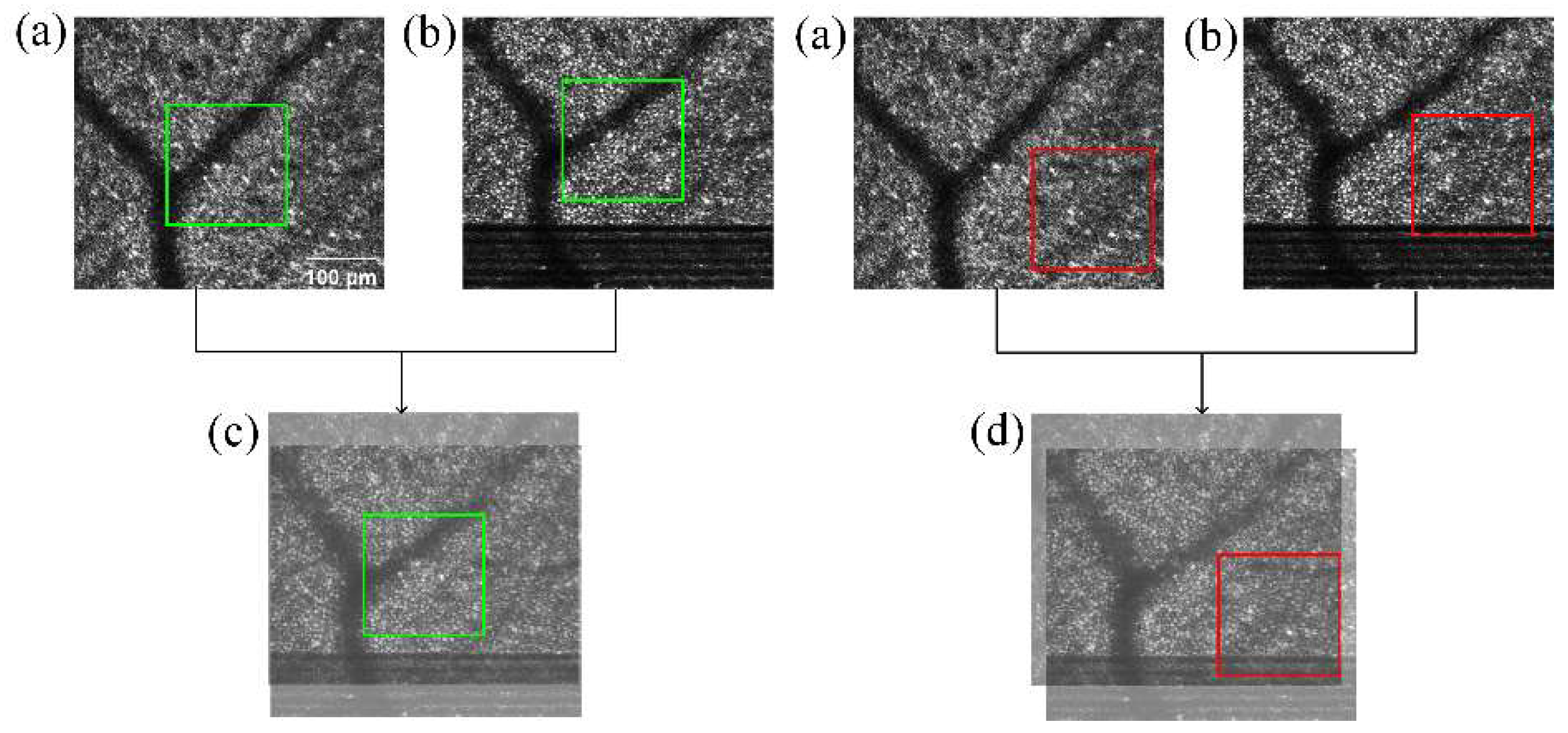
Notably, the difference between the vertical and horizontal displacements was within 10 pixels for most frames, but as shown in Figure 5c and Figure 6c, the difference reached 20 pixels or more for a few frames (the frame with the largest difference has been marked). This was caused by intra-frame distortion. Figure 7 and Figure 8 give the images with the largest vertical/horizontal displacement differences.
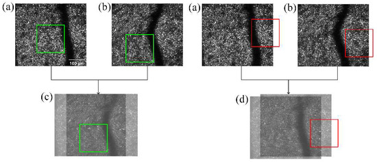
Figure 7.
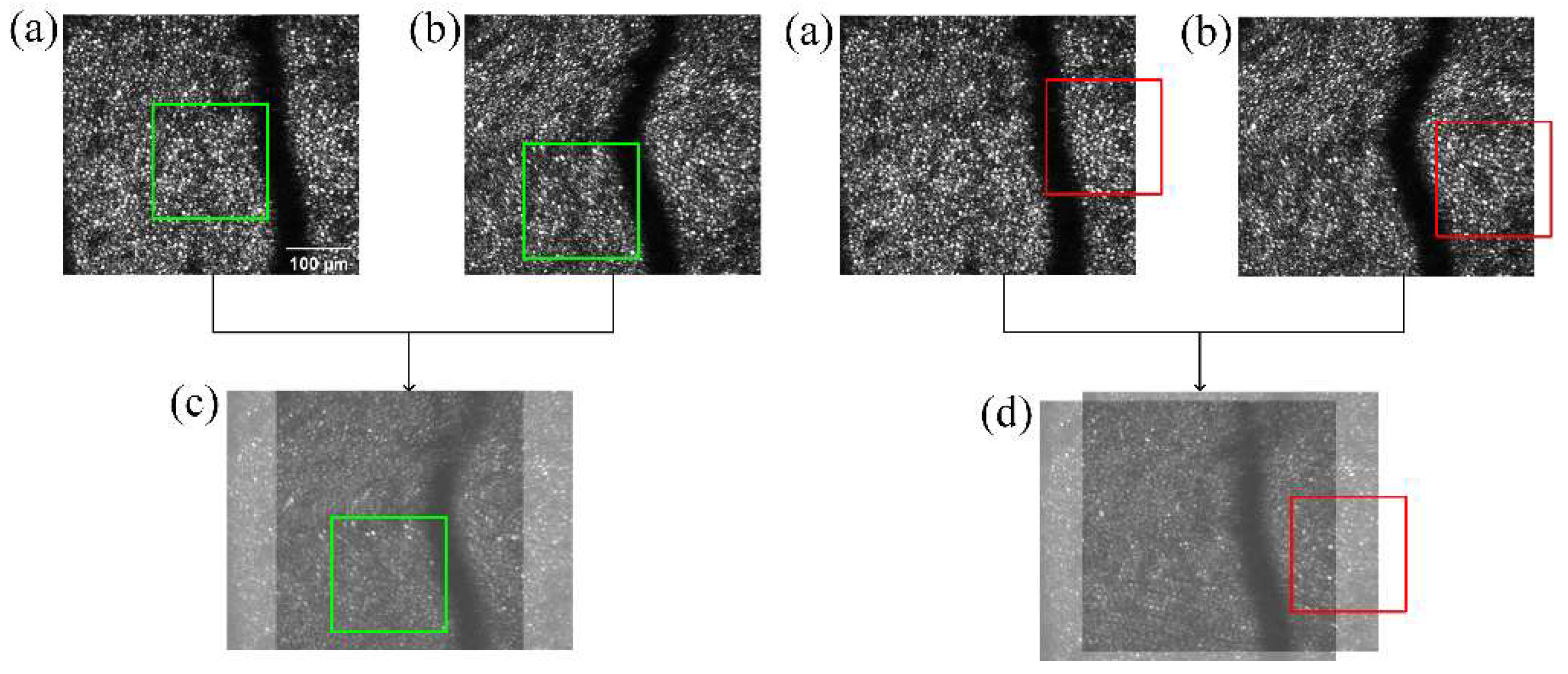
The frame with the largest vertical displacement difference; (a) is the first frame of the sequence; (b) shows the frame with the largest difference between UECO and manual registration; (c) is the result of UECO; and (d) is the result of manual registration. The green and red boxes are the references for the UECO and manual registration, respectively. For display purposes, the transparency in (c,d) was set to 50%. The scale bar is 100 µm.

Figure 8.
The frame with the largest horizontal displacement difference; (a) is the first frame of the sequence; (b) shows the frame with the largest difference between UECO and manual registration; (c) is the result of UECO; and (d) is the result of manual registration. The green and red boxes are the references for the UECO and manual registration, respectively. For display purposes, the transparency in (c,d) was set to 50%. The scale bar is 100 µm.
The red box in Figure 7 differs from that in Figure 8 because part of the reference moved out of the image. The manual registration reference differs from UECO’s reference, and the reference for manual registration was determined by the tester. There was significant intra-frame distortion in the current frame, which caused different regions of the frame to have different displacements relative to the reference. The manually registered displacement was x = 134 px, y = 88 px. The algorithm-registered displacement was x = 94 px, y = 63 px. In spite of this, both registration methods were able to stabilize the images.
3.3. Displacement Analysis under Fast Saccadic Eye Motion and Slow Drifts
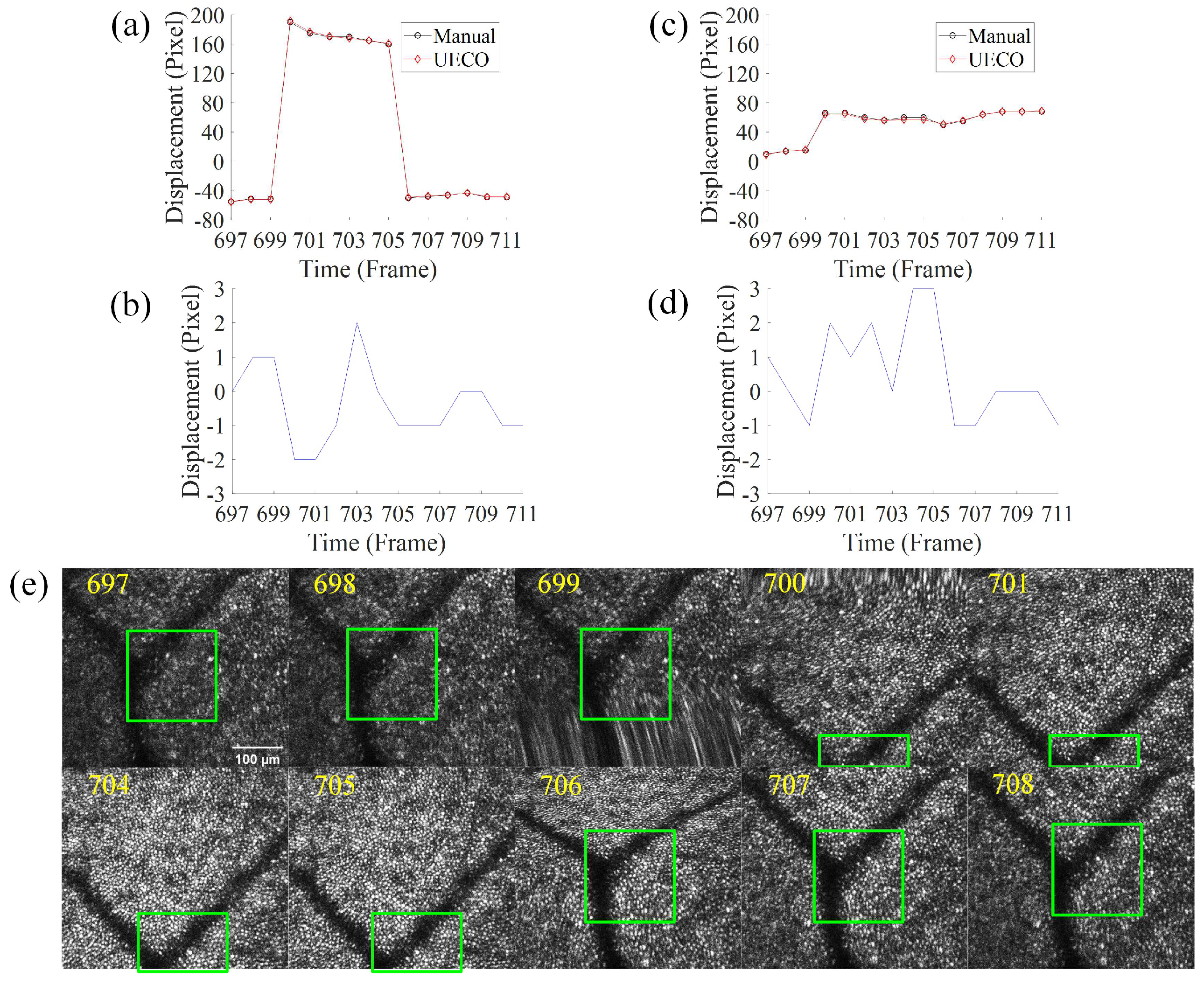
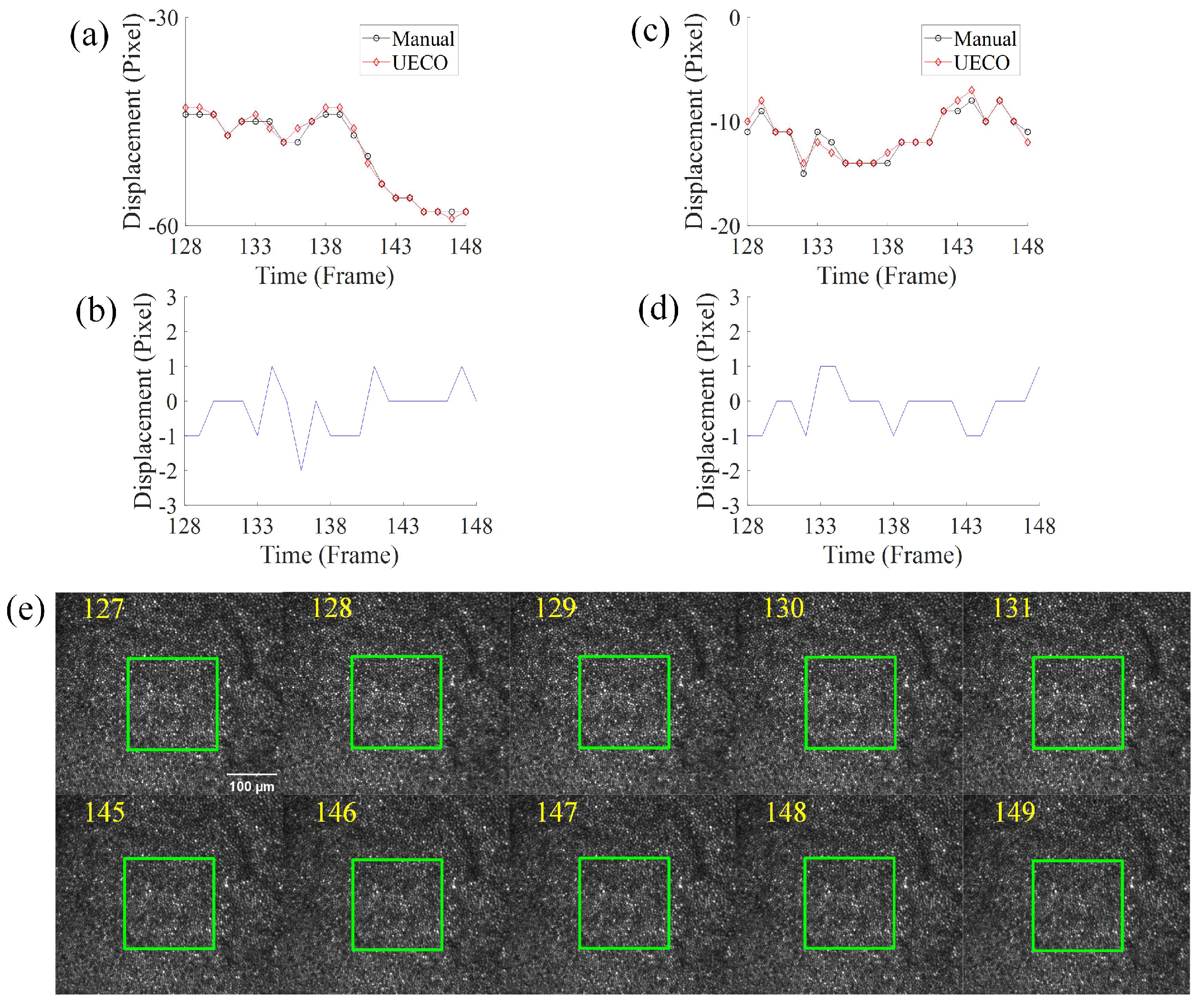
Figure 9 and Figure 10 respectively illustrate the comparison between the displacement obtained using manual registration and UECO under fast saccadic eye motion and slow drifts. When the eyes make a saccadic movement, the imaging position will change dramatically, and if the scanning rate of the AOSLO is not fast enough to keep up with the eye movement, there is a possibility of intra-frame distortion. Even in the presence of fast eye motion and intra-frame aberrations, the difference in the displacement between the algorithm and manual registration was within 3 pixels.

Figure 9.
Comparison of displacement under saccadic eye motion; (a,c) respectively show the comparison of vertical and horizontal displacement obtained by manual registration and UECO under saccadic eye motion; (b,d) are the differences in the vertical and horizontal displacement between UECO and manual registration; and (e) is 10 frames in an image sequence of saccadic eye motion. The green box is the UECO reference and the yellow text in the graph represents the current frame number. The frame number corresponds to the frame number in the original video. The scale bar is 100 µm.
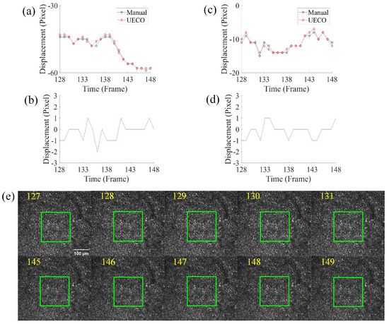
Figure 10.
Comparison of displacement under slow drifts; (a,c) respectively show the comparison of vertical and horizontal displacement obtained by manual registration and UECO under slow drifts; (b,d) are the differences in the vertical and horizontal displacement between UECO and manual registration; and (e) is 10 frames in an image sequence of slow drifts. The green box is the UECO reference and the yellow text in the graph represents the current frame number. The frame number corresponds to the frame number in the original video. The scale bar is 100 µm.
3.4. Comparison with Cross-Correlation-Based Method
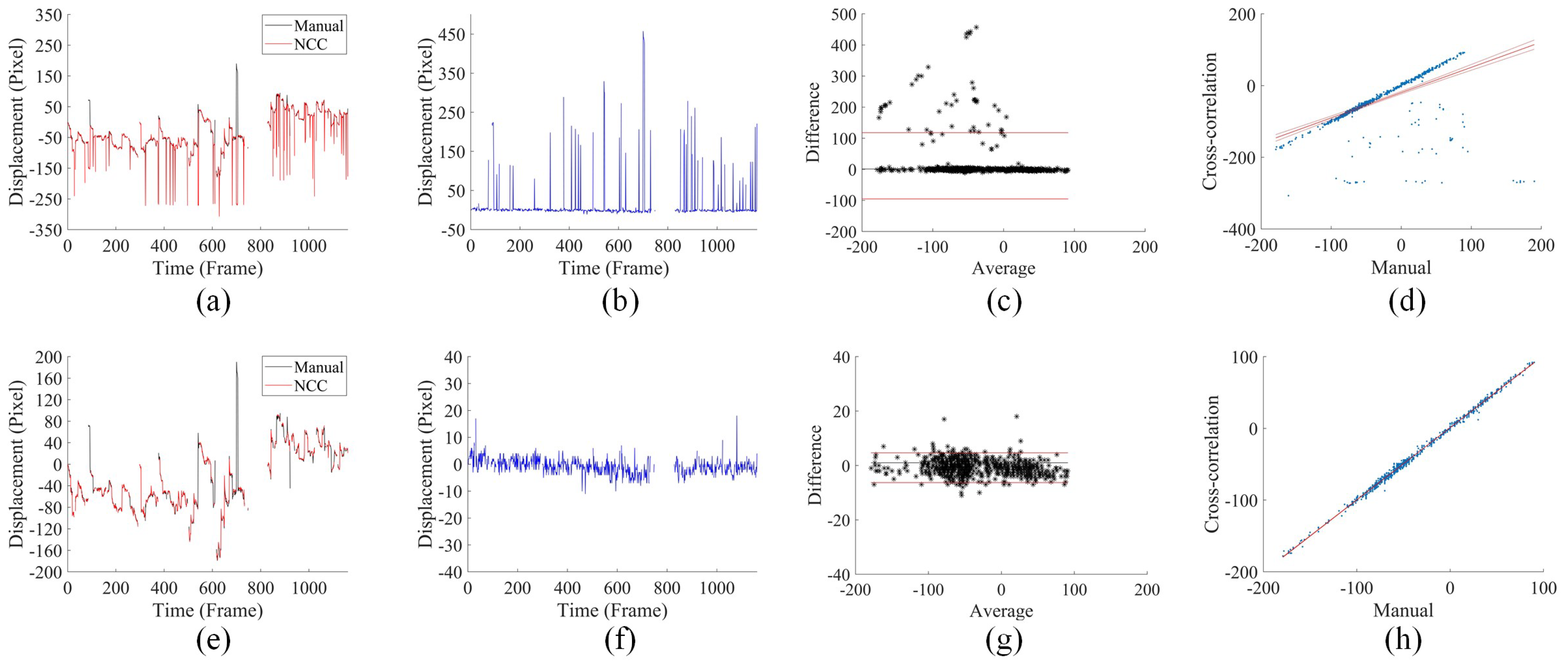
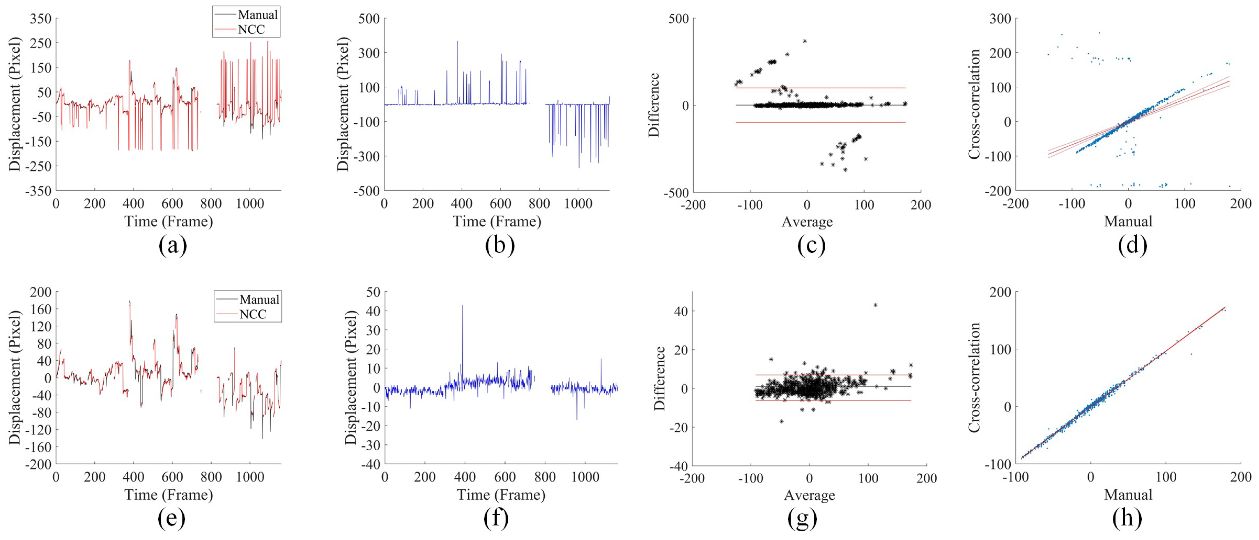
We compared the displacements calculated by UECO and a cross-correlation-based method (normalized cross-correlation, NCC) [43] with those of manual registration.
We not only compared all the displacements calculated by the cross-correlation-based method (including the wrong data due to saccadic eye motion), but also compared again with the displacement without a calculation failure (displacement within the accuracy range). Figure 11 and Figure 12 show the comparison of the displacement obtained by cross-correlation-based methods and manual registration. The mean difference in the vertical and horizontal displacement between the cross-correlation-based method and manual registration was 11.39 pixels and 0.75 pixels, respectively, with a 95% confidence interval of (−95.1 px, 117.88 px) and (−97.79 px, 99.2 px). The Pearson correlation coefficients were 0.61 and 0.5, respectively. After removing the data that failed to calculate, the mean difference in the vertical and horizontal displacement between the cross-correlation-based method and manual registration was −0.81 pixels and 0.35 pixels, respectively, with a 95% confidence interval of (−6.29 px, 4.61 px) and (−6.25 px, 6.94 px). The Pearson correlation coefficients were 0.99 and 0.99, respectively.

Figure 11.
Vertical displacement comparison chart; (a) shows the comparison of vertical displacement obtained by cross-correlation-based methods and manual registration; (b) is the difference between the two methods; and (c) is the Bland–Altman plot. The black line is the mean difference of the two methods. Red lines indicate the 95% confidence interval (mean 1.96 standard deviation). The Pearson correlation coefficient curve is shown in (d), and (e–h) show the results after removal of the wrong displacement. The frame number in the x-axis corresponds to the frame number in the original video.
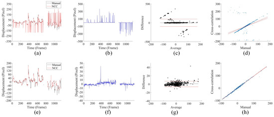
Figure 12.
Horizontal displacement comparison chart; (a) shows the comparison of vertical displacement obtained by cross-correlation-based methods and manual registration; (b) is the difference between the two methods; and (c) is the Bland–Altman plot. The black line is the mean difference of the two methods. Red lines indicate the 95% confidence interval (mean 1.96 standard deviation). The Pearson correlation coefficient curve is shown in (d), and (e–h) show the results after removal of the wrong displacement. The frame number in the x-axis corresponds to the frame number in the original video.
3.5. Comparison of the Accuracy of Cross-Correlation-Based Method and UECO
As shown in Table 1 and Table 2, we present the accuracy (mean standard deviation) of UECO and NCC. The second and third columns represent the accuracy for saccadic eye motion and slow drifts; the fourth column represents the total accuracy.

Table 1.
The accuracy of vertical displacement.

Table 2.
The accuracy of horizontal displacement.
NCC could not identify and distinguish images with saccades, and it needed to manually identify and distinguish images with saccades, which led to a low total accuracy for NCC. After the removal of the displacement that failed to calculate, the accuracy was still not as good as that of UECO. In addition, NCC was also less accurate than UECO under slow drifts.
3.6. AOSLO Image Stabilization Results
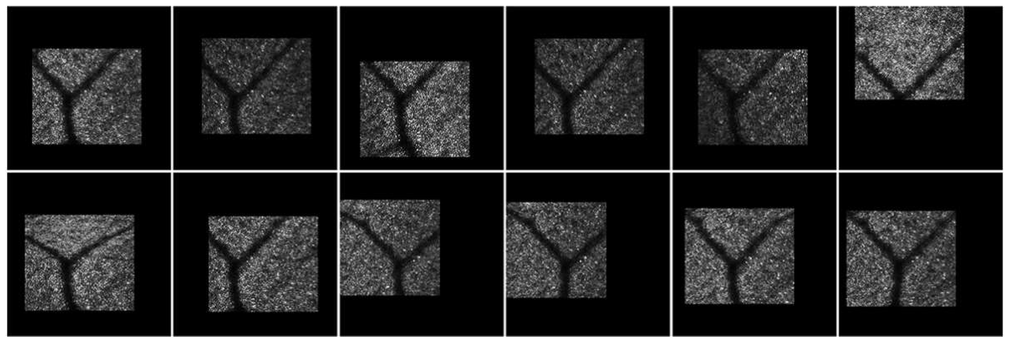
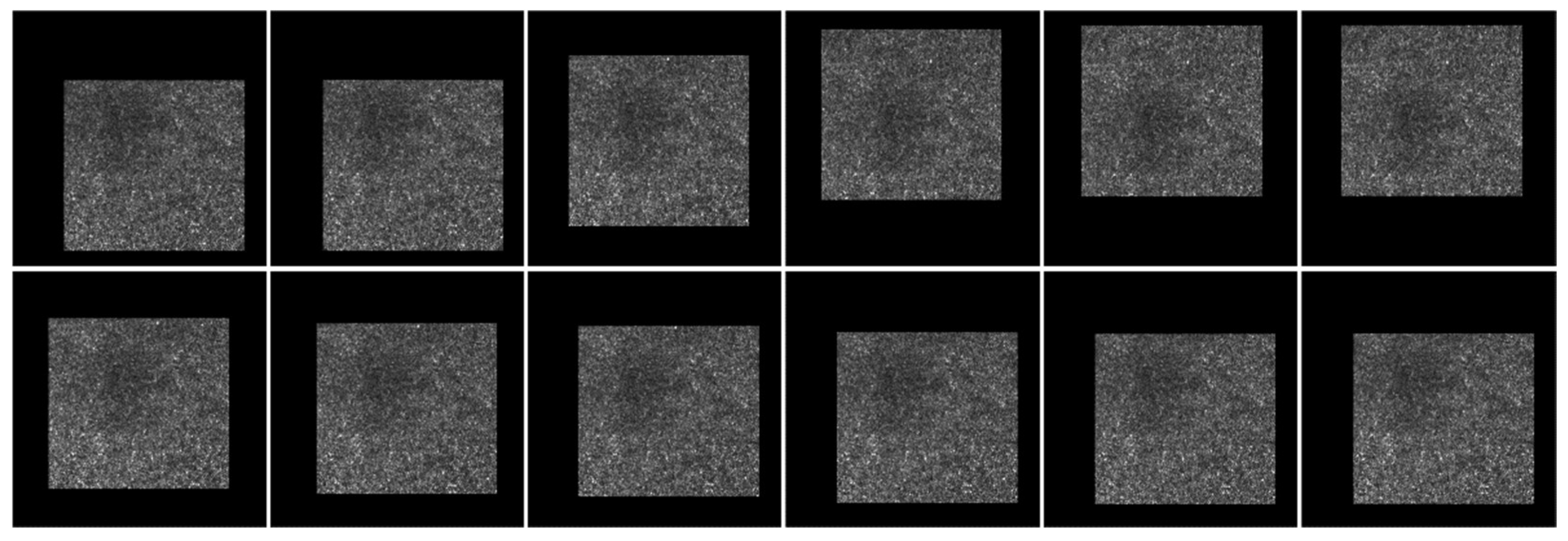
Figure 13, Figure 14, Figure 15 and Figure 16 show the results of the UECO for image stabilization. For display purposes, the image areas that moved outside the canvas were trimmed off. The original videos and the videos after stabilization are presented in the Supplementary Materials.
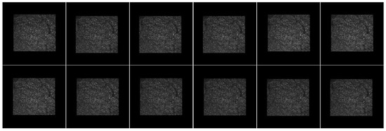
Figure 13.
AOSLO image stabilization results under slow drifts. The first image is the first frame in the sequence.

Figure 14.
AOSLO image stabilization results under saccadic eye motion. The first image is the first frame in the sequence.
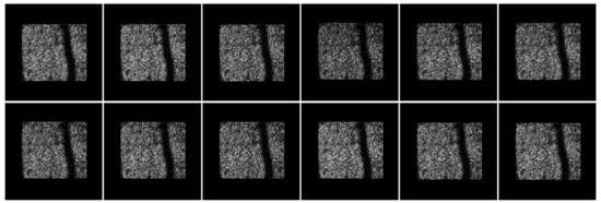
Figure 15.
AOSLO image stabilization results under slow drifts. The first image is the first frame in the sequence.

Figure 16.
AOSLO images with fovea stabilization results. The first image is the first frame in the sequence.
4. Discussion
An AOSLO is greatly affected by eye motion, and continual eye motion will cause distortions both within the frame (intra-frame) and between frames (inter-frame). To overcome eye motion, we proposed an automatic image stabilization algorithm. UECO is based on a deep-learning network; this algorithm enabled the removal of images with blinks and the correction of images with saccades. When the reference was lost due to intra-frame distortion or a change in the imaging position, UECO reset the training set and reselected the reference. Strip-based cross-correlation methods [44] enabled the removal of the intra-distortion very well, but here we only discussed the impact of inter frame motion, so we did not use strip-based cross-correlation methods to remove the intra-distortion. If it is necessary to remove intra-frame distortion, the strip-based cross-correlation method can be used.
4.1. Difference in Experiments
The manual registration reference differed from UECO’s reference, and there was a difference between the displacement calculated for UECO and manual registration due to intra-frame distortion in some images. The UECO was robust and calculated displacements correctly, even if there were significant distortions within the frame. If manual registration and UECO selected the same reference, the difference between manual registration and UECO would be even further reduced.
4.2. Limitation
Compared with traditional methods, UECO is time-consuming due to the high computational load associated with deep-learning algorithms. In the experiment in Section 3 (the test video had 1163 frames in total), the cross-correlation-based method took 113 s (0.1 fps), while UECO took 1717 s (1.47 fps). Therefore, UECO cannot be used for real-time image stabilization in the imaging process. In the future, we intend to optimize the deep-learning network and make it more lightweight in order to decrease its computation load and improve its speed.
At present, since we were not able to obtain patient data without permission from the hospital, our data came only from healthy subjects. Next, we will cooperate with the hospital to obtain data from patients and experiment with this data.
5. Conclusions
We developed a deep-learning network (VGG-16)-based algorithm for automatic image stabilization. During image stabilization, images with blinks were removed and images with saccades were corrected. To overcome the loss of the reference due to eye motion or a change in the imaging position, we proposed the method of resetting the training set. The experimental results showed that UECO was more accurate than the cross-correlation-based methods and enabled manual registration accuracy to be achieved without manual intervention.
Supplementary Materials
The following supporting information can be downloaded at: https://www.mdpi.com/article/10.3390/info13110531/s1, Video S1: The original video; Video S2: The video after stabilization; Video S3: The original video (fovea); Video S4: The video (fovea) after stabilization.
Author Contributions
Conceptualization, S.L. and B.G.; methodology, Z.J.; software, Z.J. and Y.H.; validation, J.C. and G.L.; formal analysis, X.X.; investigation, Y.H.; resources, Y.H.; data curation, Y.H. and J.L.; writing—original draft preparation, Z.J. and B.G.; writing—review and editing, B.G. and Z.J.; visualization, B.G.; supervision, J.L.; project administration, B.G., J.L. and Z.J.; funding acquisition, Y.H. and J.L. All authors have read and agreed to the published version of the manuscript.
Funding
This research was funded by the National Natural Science Foundation of China, grant number 62075235.
Institutional Review Board Statement
All subjects gave their informed consent for inclusion before they participated in the study. All procedures performed in studies involving human participants were in accordance with the ethical standards of the institutional and/or national research committee and with the Helsinki declaration and its later amendments or comparable ethical standards.
Informed Consent Statement
Informed consent was obtained from all subjects involved in the study.
Data Availability Statement
Not applicable.
Conflicts of Interest
The authors declare no conflict of interest.
References
- DeHoog, E.; Schwiegerling, J. Fundus camera systems: A comparative analysis. Appl. Opt. 2009, 48, 221–228. [Google Scholar] [CrossRef] [PubMed]
- Yao, X.; Son, T.; Ma, J. Developing portable widefield fundus camera for teleophthalmology: Technical challenges and potential solutions. Exp. Biol. Med. 2021, 247, 289–299. [Google Scholar] [CrossRef] [PubMed]
- De Boer, J.F.; Leitgeb, R.; Wojtkowski, M. Twenty-five years of optical coherence tomography: The paradigm shift in sensitivity and speed provided by Fourier domain OCT [Invited]. Biomed. Opt. Express 2017, 8, 3248–3280. [Google Scholar] [CrossRef] [PubMed]
- Liu, G.; Chen, Z. Advances in Doppler OCT. Chin. Opt. Lett 2013, 11, 011702. [Google Scholar]
- Makita, S.; Miura, M.; Azuma, S.; Mino, T.; Yamaguchi, T.; Yasuno, Y. Accurately motion-corrected Lissajous OCT with multi-type image registration. Biomed. Opt. Express 2021, 12, 637–653. [Google Scholar] [CrossRef]
- Mecê, P.; Scholler, J.; Groux, K.; Boccara, C. High-resolution in-vivo human retinal imaging using full-field OCT with optical stabilization of axial motion. Biomed. Opt. Express 2020, 11, 492–504. [Google Scholar] [CrossRef]
- Pircher, M.; Zawadzki, R.J. Review of adaptive optics OCT (AO-OCT): Principles and applications for retinal imaging [Invited]. Biomed. Opt. Express 2017, 8, 2536–2562. [Google Scholar] [CrossRef]
- Azimipour, M.; Jonnal, R.S.; Werner, J.S.; Zawadzki, R.J. Coextensive synchronized SLO-OCT with adaptive optics for human retinal imaging. Opt. Lett. 2019, 44, 4219–4222. [Google Scholar] [CrossRef]
- Bower, A.J.; Liu, T.; Aguilera, N.; Li, J.; Liu, J.; Lu, R.; Giannini, J.P.; Huryn, L.A.; Dubra, A.; Liu, Z.; et al. Integrating adaptive optics-SLO and OCT for multimodal visualization of the human retinal pigment epithelial mosaic. Biomed. Opt. Express 2021, 12, 1449–1466. [Google Scholar] [CrossRef]
- Felberer, F.; Rechenmacher, M.; Haindl, R.; Baumann, B.; Hitzenberger, C.K.; Pircher, M. Imaging of retinal vasculature using adaptive optics SLO/OCT. Biomed. Opt. Express 2015, 6, 1407–1418. [Google Scholar] [CrossRef]
- Pircher, M.; Baumann, B.; Götzinger, E.; Sattmann, H.; Hitzenberger, C.K. Simultaneous SLO/OCT imaging of the human retina with axial eye motion correction. Opt. Express 2007, 15, 16922–16932. [Google Scholar] [CrossRef] [PubMed]
- Pircher, M.; Götzinger, E.; Sattmann, H.; Leitgeb, R.A.; Hitzenberger, C.K. In vivo investigation of human cone photoreceptors with SLO/OCT in combination with 3D motion correction on a cellular level. Opt. Express 2010, 18, 13935–13944. [Google Scholar] [CrossRef] [PubMed]
- Roorda, A.; Romero-Borja, F.; Donnelly Iii, W.; Queener, H.; Hebert, T.; Campbell, M. Adaptive optics scanning laser ophthalmoscopy. Opt Express 2002, 10, 405–412. [Google Scholar] [CrossRef] [PubMed]
- Migacz, J.V.; Otero-Marquez, O.; Zhou, R.; Rickford, K.; Murillo, B.; Zhou, D.B.; Castanos, M.V.; Sredar, N.; Dubra, A.; Rosen, R.B.; et al. Imaging of vitreous cortex hyalocyte dynamics using non-confocal quadrant-detection adaptive optics scanning light ophthalmoscopy in human subjects. Biomed. Opt. Express 2022, 13, 1755–1773. [Google Scholar] [CrossRef]
- Ferguson, R.D.; Zhong, Z.; Hammer, D.X.; Mujat, M.; Patel, A.H.; Deng, C.; Zou, W.; Burns, S.A. Adaptive optics scanning laser ophthalmoscope with integrated wide-field retinal imaging and tracking. JOSA A 2010, 27, A265–A277. [Google Scholar] [CrossRef] [PubMed]
- Bakker, E.; Dikland, F.A.; van Bakel, R.; Andrade De Jesus, D.; Sánchez Brea, L.; Klein, S.; van Walsum, T.; Rossant, F.; Farías, D.C.; Grieve, K.; et al. Adaptive optics ophthalmoscopy: A systematic review of vascular biomarkers. Surv. Ophthalmol. 2022, 67, 369–387. [Google Scholar] [CrossRef] [PubMed]
- Harmening, W.M.; Tuten, W.S.; Roorda, A.; Sincich, L.C. Mapping the Perceptual Grain of the Human Retina. J. Neurosci. Methods 2014, 34, 5667–5677. [Google Scholar] [CrossRef]
- Martin, J.A.; Roorda, A. Direct and noninvasive assessment of parafoveal capillary leukocyte velocity. Ophthalmology 2005, 112, 2219–2224. [Google Scholar] [CrossRef]
- Guevara-Torres, A.; Joseph, A.; Schallek, J.B. Label free measurement of retinal blood cell flux, velocity, hematocrit and capillary width in the living mouse eye. Biomed. Opt. Express 2016, 7, 4228–4249. [Google Scholar] [CrossRef]
- Lu, J.; Gu, B.; Wang, X.; Zhang, Y. High-speed adaptive optics line scan confocal retinal imaging for human eye. PLoS ONE 2017, 12, e0169358. [Google Scholar] [CrossRef]
- Lu, J.; Gu, B.; Wang, X.; Zhang, Y. High speed adaptive optics ophthalmoscopy with an anamorphic point spread function. Opt. Express 2018, 26, 14356–14374. [Google Scholar] [CrossRef] [PubMed]
- Salmon, A.E.; Cooper, R.F.; Langlo, C.S.; Baghaie, A.; Dubra, A.; Carroll, J. An Automated Reference Frame Selection (ARFS) Algorithm for Cone Imaging with Adaptive Optics Scanning Light Ophthalmoscopy. Transl. Vis. Sci. Technol. 2017, 6, 9. [Google Scholar] [CrossRef] [PubMed]
- Arathorn, D.W.; Stevenson, S.B.; Yang, Q.; Tiruveedhula, P.; Roorda, A. How the unstable eye sees a stable and moving world. J. Vis 2013, 13, 22. [Google Scholar] [CrossRef] [PubMed]
- Arathorn, D.W.; Yang, Q.; Vogel, C.R.; Zhang, Y.; Tiruveedhula, P.; Roorda, A. Retinally stabilized cone-targeted stimulus delivery. Opt. Express 2007, 15, 13731–13744. [Google Scholar] [CrossRef]
- Braaf, B.; Vienola, K.V.; Sheehy, C.K.; Yang, Q.; Vermeer, K.A.; Tiruveedhula, P.; Arathorn, D.W.; Roorda, A.; de Boer, J.F. Real-time eye motion correction in phase-resolved OCT angiography with tracking SLO. Biomed. Opt. Express 2013, 4, 51–65. [Google Scholar] [CrossRef]
- Hammer, D.X.; Ferguson, R.D.; Magill, J.C.; White, M.A.; Elsner, A.E.; Webb, R.H. Tracking scanning laser ophthalmoscope (TSLO). Ophthalmic Technol. 2003, 4951, 208–217. [Google Scholar]
- Kowalski, B.; Huang, X.; Steven, S.; Dubra, A. Hybrid FPGA-CPU pupil tracker. Biomed. Opt. Express 2021, 12, 6496–6513. [Google Scholar] [CrossRef]
- Sheehy, C.K.; Yang, Q.; Arathorn, D.W.; Tiruveedhula, P.; de Boer, J.F.; Roorda, A. High-speed, image-based eye tracking with a scanning laser ophthalmoscope. Biomed. Opt. Express 2012, 3, 2611–2622. [Google Scholar] [CrossRef]
- Zhang, J.; Yang, Q.; Saito, K.; Nozato, K.; Williams, D.R.; Rossi, E.A. An adaptive optics imaging system designed for clinical use. Biomed. Opt. Express 2015, 6, 2120–2137. [Google Scholar] [CrossRef]
- Chan, H.P.; Samala, R.K.; Hadjiiski, L.M.; Zhou, C. Deep Learning in Medical Image Analysis. Adv. Exp. Med. Biol. 2020, 1213, 3–21. [Google Scholar] [CrossRef]
- De Silva, T.; Chew, E.Y.; Hotaling, N.; Cukras, C.A. Deep-learning based multi-modal retinal image registration for the longitudinal analysis of patients with age-related macular degeneration. Biomed. Opt. Express 2021, 12, 619–636. [Google Scholar] [CrossRef] [PubMed]
- Simonyan, K.; Zisserman, A.J.C. Very Deep Convolutional Networks for Large-Scale Image Recognition. arXiv 2015, arXiv:1409.1556. [Google Scholar]
- Bolme, D.S.; Beveridge, J.R.; Draper, B.A.; Lui, Y.M. Visual object tracking using adaptive correlation filters. In Proceedings of the 2010 IEEE Computer Society Conference on Computer Vision and Pattern Recognition, San Francisco, CA, USA, 13–18 June 2010; pp. 2544–2550. [Google Scholar]
- Wang, Y.; He, Y.; Wei, L.; Li, X.; Yang, J.; Zhou, H.; Zhang, Y. Bimorph deformable mirror based adaptive optics scanning laser ophthalmoscope for retina imaging in vivo. Chin. Opt. Lett. 2017, 15, 121102. [Google Scholar] [CrossRef]
- Danelljan, M.; Bhat, G.; Khan, F.S.; Felsberg, M. ECO: Efficient Convolution Operators for Tracking. In Proceedings of the 2017 IEEE Conference on Computer Vision and Pattern Recognition (CVPR), Honolulu, HI, USA, 21–26 July 2017; pp. 6931–6939. [Google Scholar]
- Chatfield, K.; Simonyan, K.; Vedaldi, A.; Zisserman, A. Return of the Devil in the Details: Delving Deep into Convolutional Nets. arXiv 2014, arXiv:1405.3531. [Google Scholar]
- Deng, J.; Dong, W.; Socher, R.; Li, L.J.; Kai, L.; Li, F.-F. ImageNet: A large-scale hierarchical image database. In Proceedings of the 2009 IEEE Conference on Computer Vision and Pattern Recognition, Miami, FL, USA, 20–25 June 2009; pp. 248–255. [Google Scholar]
- Kristan, M.; Leonardis, A.; Matas, J.; Felsberg, M.; Pflugfelder, R.; Čehovin, L.; Vojíř, T.; Häger, G. (Eds.) The Visual Object Tracking VOT2016 Challenge Results; Springer International Publishing: Cham, Switzerland, 2016. [Google Scholar]
- Mueller, M.; Smith, N.; Ghanem, B. (Eds.) A Benchmark and Simulator for UAV Tracking2016; Springer International Publishing: Cham, Switzerland, 2016. [Google Scholar]
- Wu, Y.; Lim, J.; Yang, M. Object Tracking Benchmark. IEEE Trans. Pattern Anal. Mach. Intell. 2015, 37, 1834–1848. [Google Scholar] [CrossRef] [PubMed]
- Liang, P.; Blasch, E.; Ling, H. Encoding Color Information for Visual Tracking: Algorithms and Benchmark. IEEE Trans. Image Process. 2015, 24, 5630–5644. [Google Scholar] [CrossRef]
- Otsu, N. A Threshold Selection Method from Gray-Level Histograms. IEEE Trans. Syst. Man Cybern. 1979, 9, 62–66. [Google Scholar] [CrossRef]
- Briechle, K.; Hanebeck, U.D. Template matching using fast normalized cross correlation. In Proceedings of the SPIE Defense + Commercial Sensing, Orlando, FL, USA, 20 March 2001. [Google Scholar]
- Yang, Q.; Zhang, J.; Nozato, K.; Saito, K.; Williams, D.R.; Roorda, A.; Rossi, E.A. Closed-loop optical stabilization and digital image registration in adaptive optics scanning light ophthalmoscopy. Biomed. Opt. Express 2014, 5, 3174–3191. [Google Scholar] [CrossRef]
Publisher’s Note: MDPI stays neutral with regard to jurisdictional claims in published maps and institutional affiliations. |
© 2022 by the authors. Licensee MDPI, Basel, Switzerland. This article is an open access article distributed under the terms and conditions of the Creative Commons Attribution (CC BY) license (https://creativecommons.org/licenses/by/4.0/).


