
Extraction and Analysis of Social Networks Data to Detect Traffic Accidents


Abstract
1. Introduction
2. Literature Review
2.1. Analysis of Traffic Accidents
2.2. Information on Traffic Accidents Posted on Social Media
2.3. Methods for Incident Extraction from Social Media
2.3.1. Automatic Classification of Tweets Related to Accidents
- Preprocessing: In this phase, the posts are received, cleaned and normalized, dividing the sentences into words or segments called tokens (tokenization). Web links or URLs, user mentions (@), empty words or stopwords, special characters and numbers are eliminated. Finally, the words are reduced according to their lemma (lemmatization) or their stem (stemming).
- Feature extraction: The sentences generated in the previous step are represented as features or vectors to improve the performance of the mathematical models. In the literature, the TD-IDF technique has been implemented, which represents the frequency of the words in the tweet with respect to the number of tweets in the corpus [27,29]. Another technique being used is word2vec, which is a trained neural network that generates smaller semantic arrays taking into account the context of the words within the sentence [24,30].
- Automatic classification: From the results of the previous phase, a machine learning model is built to determine whether a tweet is related to an incident or not; some algorithms used in the literature are naive bayes [11,25], support vector machine [21,23,28] and convolutional neural networks [30]. Each model has different parameters that must be configured to obtain better results; these parameters are searched through an optimized intensive search, such as the grid search method.
2.3.2. Named Entity Recognition
- Preprocessing. Some URLs, emoticons and special characters are deleted. The @usernames and #hashtags may contain location information and some authors do not eliminate them. These expressions are generally formed by two or three words without spaces, so a method is applied to expand them [34,35]. Furthermore, spelling errors and abbreviations commonly used in social media are corrected [33]. In order to recognize entities, stopwords are not eliminated because these words are key to understand the context of the following word and avoid ambiguities.
- Entity recognition. There are different techniques that can be employed to extract location entities in tweets. In general, they are classified into two types: based-rules and sequence labeling. Some authors use a hybrid of both techniques [11,33,35,36,37]. The main difference lies in the use of resources external to the text content itself, such as based-rules techniques that build dictionaries of terms, toponymies and metonymies; local Gazetteers; a set of rules or a list of regular expressions. On the other hand, Sequence Labeling techniques use supervised machine learning methods, using only a set of labeled features and data from text, thus training, learning and generalizing on unseen data. The best performing models for the sequence labeling task in social networks are CRF [37], BiLSTM [31] and BiLSTM+CRF [32].
2.3.3. Geocoding
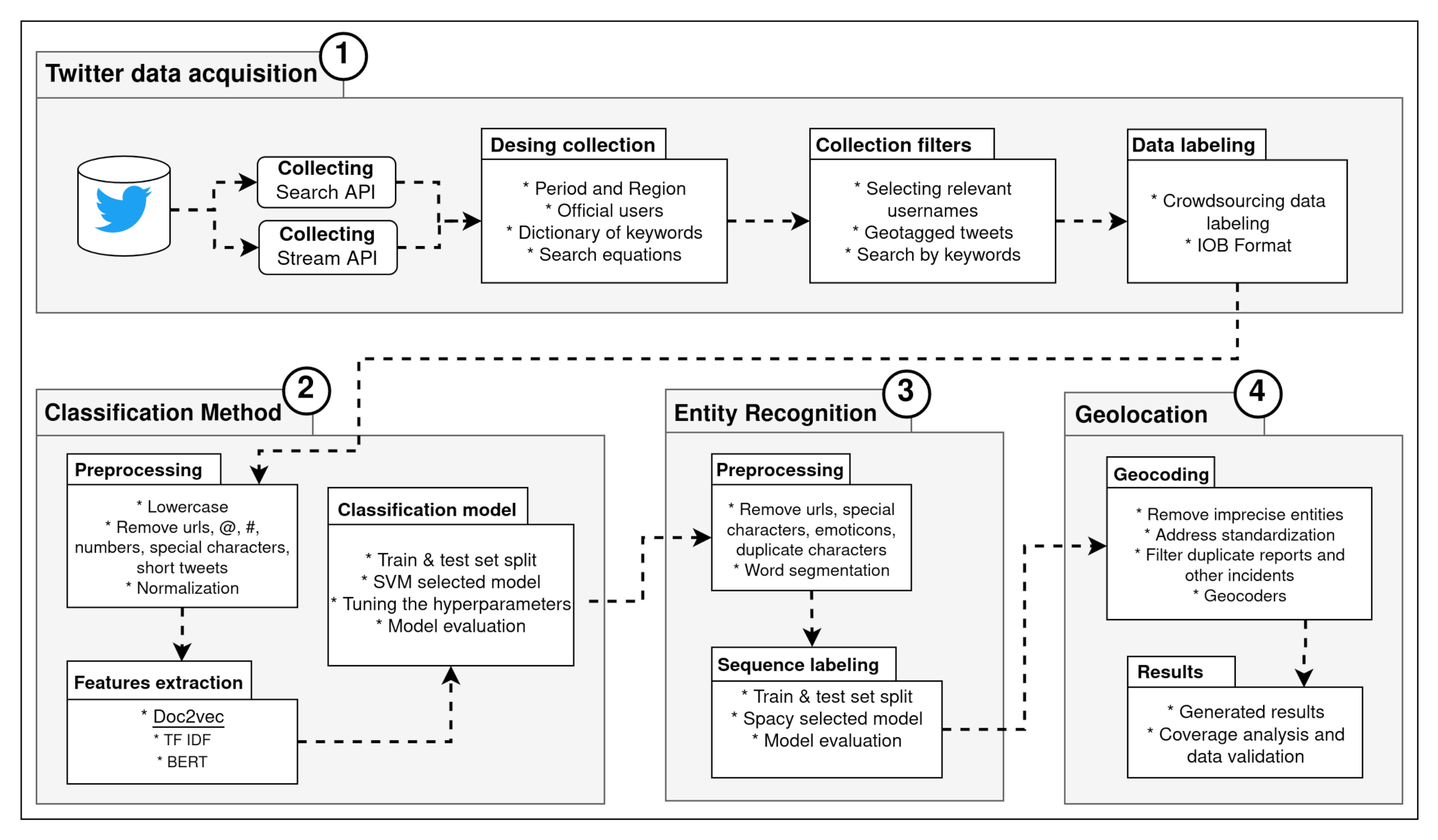
3. Materials and Methods
3.1. Twitter Data Acquisition
3.1.1. Design Collection
- Period and region. The tweets in Spanish correspond to the city of Bogota, Colombia and were collected for ten months: from October to December 2018 and from January to July 2019.
- Official users. Given the importance of traffic reports in the city of Bogota, the official user accounts shown in Table 1 are selected. In this table the user profiles represent some important sector such as @BogotaTransito which belongs to Bogota city transit authority, @CIVICOSBOG and @RedapBogota belong to civic organizations, @Cititv which is a news channel account and @transmilenio and @rutassitp belong to public transport services.
- Keywords dictionary. The Twitter API enables to extract tweets based on a keyword match. In order to determine the list of keywords, the words (sequences of words called n-grams) with the highest occurrence among hand-picked documents, reports and tweets related to traffic accidents are manually extracted.
- Search equations. Some search equations are created based on the word dictionary to optimize the extraction. As seen in Table 2, these equations include the word exceptions to discard irrelevant tweets; the “-” sign indicates these words should be excluded. Some user accounts or hashtags are also included in the search.
3.1.2. Collection Filters
- Stream Bogotá. Query to extract tweets posted in Bogota with Stream API. The free version only extracts 1% of the tweets. Furthermore, it only provides the tweets with the geotag option enabled or those posted from cell phones with GPS enabled.
- Stream Follow/Timeline User. Tweets collected using Twitter Stream API. One or several users are selected; and an automatic download is started the moment the user posts a tweet or someone tags him/her in a comment.
- Search Token. Tweets are collected using Twitter Search API. In this case, the search equations defined in Table 2 are used; additionally, the results are filtered for Bogotá and Spanish.
- Search Timeline User. Tweets are collected from five selected users from Table 1 using Twitter Search API. (@BogotaTransito, @Citytv, @RedapBogota, @WazeTrafficBog, @CIVICOSBOG). The tweets posted in their timelines are downloaded, and the API allows to extract the user’s tweet history.
3.1.3. Data Labeling
Crowdsourcing Data Labeling for Classification
Sequential Data Tagging
3.2. Classification Method
3.2.1. Preprocessing
- A
- Conversion to lowercase: Since word dictionaries are case sensitive, all words in tweets were shifted to lowercase.
- B
- Cleaning of non-alphabetic characters: Special characters, e-mail addresses, URLs, including @ and # symbols that are popular on Twitter were removed.
- C
- Normalization with lemmatization: In Spanish, words have variations and are conjugated in different forms. To find a more generalized pattern, a normalization process was applied to tweets, which consisted of reducing the word to its original lemma. Another form of normalization is stemming which, instead of reducing it to its lemma, it reduces the word to its stem. It consists of removing and replacing suffixes from the word stem. In the following sections, the performance of the proposed method is evaluated by comparing lemmatization and stemming.
- D
- Tweets whose word count or token length was fewer than three after performing the steps above are discarded.
3.2.2. Features Extraction
3.2.3. Classification Model
3.3. Entity Recognition
3.3.1. Preprocessing
- Remove unnecessary ASCII codes, URLs and line breaks.
- Remove special characters and emoticons, except for punctuation marks and accents.
- Delete letters or punctuation marks that repeat consecutively. If a letter is repeated more than two times in a row, the other letters are deleted. For example, “goooool” is replaced by “gol” (goal in English). In the case of symbols, if they are repeated more than three times in a row, they are deleted.
Word Segmentation in Social Media
- A
- Dataset. A corpus with 400 K unigrams was built using the Spanish dataset of Cañete et al. [42] with about three billion tokens and the in-house dataset extracted from Twitter with 76 million tokens.
- B
- Cleaning and normalization. The same preprocessing mentioned above was applied. In this case, the accent was removed from the words so they did not have any accent. Each text was divided into unigrams to create a dictionary.
- C
- Naive Bayes-based language model. With the dataset, a language model was created, which predicted several word segmentations and the most probable one was selected.
3.3.2. Sequence Labeling
3.4. Geolocation
- A
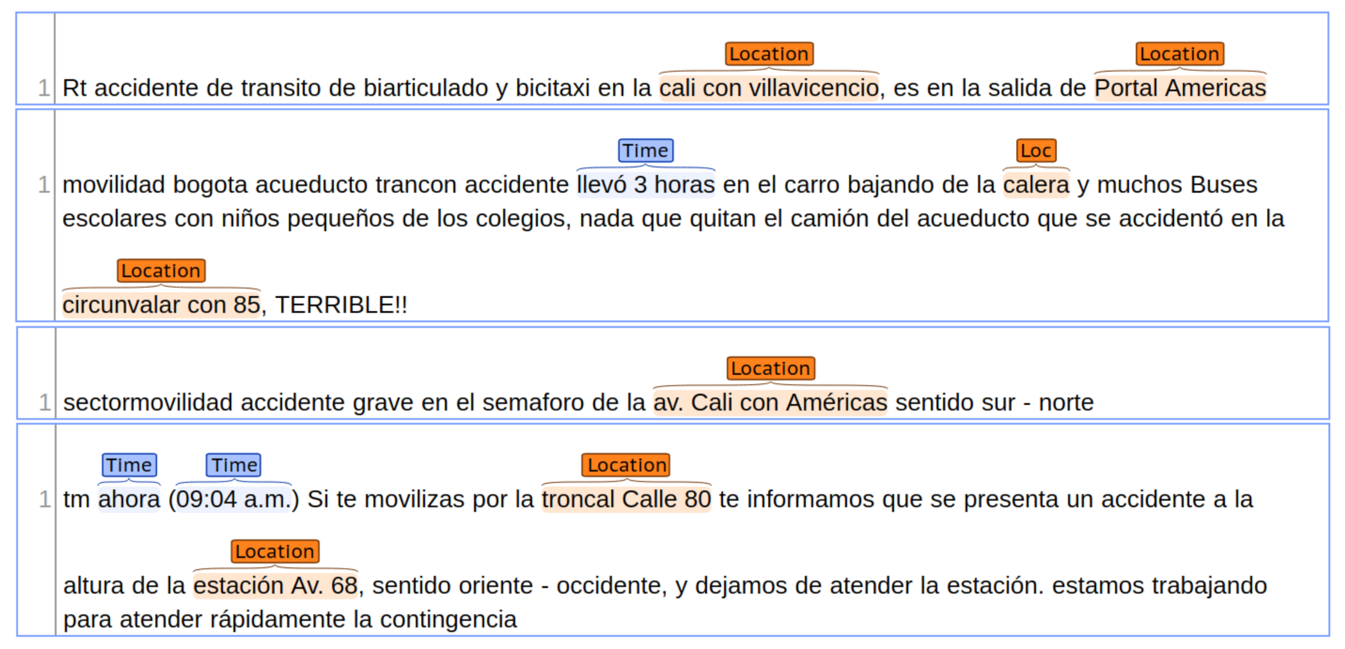
- Remove tweets with inaccurate location entities. Some tweets make reference to more than one location or include vague references to the location of the incident without specifying further details, which makes it difficult to geolocate the coordinates. For this reason, it was decided to apply the following two rules to filter these tweets. The underlined text refers to the location entities detected by the method.
- Discard tweets with fewer than four words in the detected location. For example, “Accidente en Calle 22 trafico bogota, the entity “calle 22” does not provide sufficient information.
- Discard tweets with more than four recognized location entities. Tweets mentioning different locations or addresses in the report. For example, -“Calle 34 trancada al Oriente desde la calle 26 hasta la carrera 13 -choque en la Glorieta de la Avenida Primero de Mayo con carrera 68, is a tweet with two traffic reports in different locations.
- B
- Address Standardization. The addresses or locations detected in the tweets lack a formal language, thus limiting the effectiveness of the geocoders. Some drawbacks are the use of abbreviations, different toponymies for the same place and lack of precision in the address or incomplete place names. These problems motivated to use a method to enrich and standardize the locations detected in the tweets messages. For this reason, the Libpostal library was used (repository available on https://github.com/openvenues/libpostal, accessed on 20 November 2021). This library allowed to adapt the dictionaries of words, toponymies, abbreviations and other modifications made to adapt to the particularities of Bogota. Finally, Libpostal can transform a location recognized as “cl 72 * cra 76” → “BOGOTA AVENIDA CALLE 72 CARRERA 76”.
- C
- Filtering duplicate reports and other incidents. To reduce the cost of using paid geocoders such as Google Maps API, which charge per query, duplicate reports and noise present in Twitter were first removed. The objective was to extract additional information on Twitter and not duplicate existing information. At this point, tweets with similar locations—extracted in the previous step—and occurring at the same address in a 1-h time window (before and after) were removed. In addition, to filter tweets from other events or incidents, a final selection was made by matching keywords related to accidents, thus eliminating non-relevant reports.
- D
- Geocoders. Once the addresses were standardized, a geocoder returned a geographic coordinate. An app called batch geocode (Available on https://github.com/GISforHealth/batch_geocode accessed on 20 November 2021 (GISforHealth’s Github repository)) was used, which combines resources available on Google, OpenStreetMap and Geonames. Up to four results were fetched per resource and the geocoding tool automatically assigned a coordinate if all points fall within a zone of influence.
4. Results
4.1. Case Study: Traffic Accident Report in Bogotá D.C. (Colombia)
4.2. Data
4.2.1. Data for Classification Method
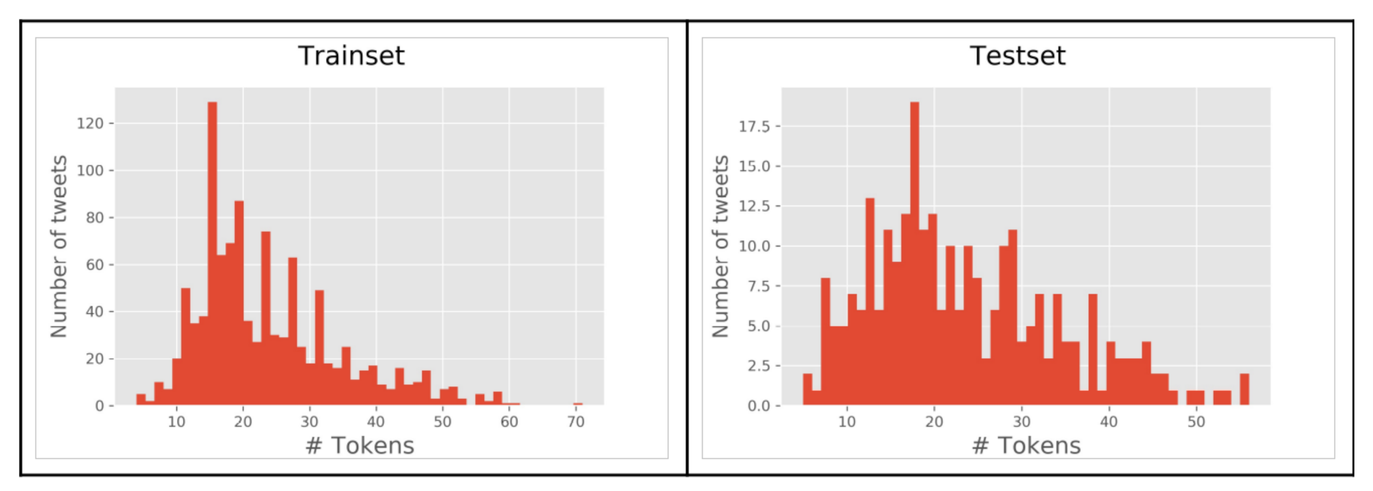
4.2.2. Data for Entity Recognition
4.3. Experiment
4.3.1. Evaluation Metrics
Classification
Sequence Labeling
4.3.2. Preprocessing
Lemmatization vs. Stemming
Stopwords
4.3.3. Embedding Methods
DBOW/doc2vec
- Splitting the tweet into unigrams.
- Vector size generated in 200 columns.
- Learning rate 0.025 and stochastic gradient descent optimizer.
- Context window size to five—that is, counting two neighboring words to the right and left of the target word.
- Ignoring words when the number of occurrences is fewer than four.
- Twelve iterations and fifteen training epochs.
TF-IDF
- max_df, to ignore words or tokens with higher frequency.
- max_feautres, to determine the size of the resulting vector.
- min_df, to ignore words with lower frequency.
- ngram_range, minimum and maximum range of N grams for vocabulary construction.
BERT
- The @usernames were replaced by the [MASK] label.
- URLs, repeated continuous characters, the RT word and special characters except for punctuation marks were removed. In this case, BERT assigns a special mask.
- Hashtags or # were expanded.
4.3.4. Comparing the Classification Methods
SVM
Naive Bayes
Random Forest
Neural Network
4.3.5. Comparing the Sequence Labeling Models
CRF
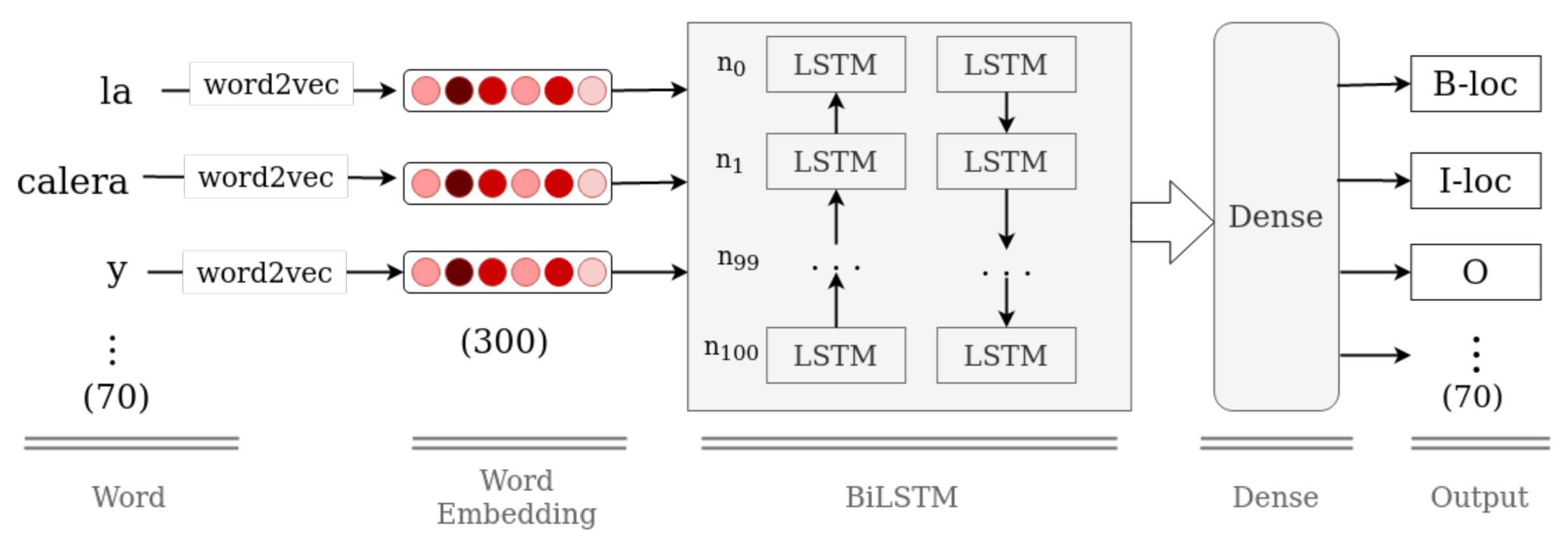
BiLSTM
BiLSTM + CRF
Spacy
4.4. Results
4.4.1. Evaluation on Classification Models
4.4.2. Evaluation on Named Entity Recognition Models
4.4.3. Comparison of Literature Related
Classification
Location Recognition
4.4.4. Analysis of the Processing of Tweets in Bogotá
4.5. Analysis of Traffic Accident Coverage between Twitter and Official Source
4.5.1. Map-Matched with Official Accident Record
- In some cases, there is a difference of up to 1 h before or after between the official source and Twitter. The official hour is conditioned by the witnesses’ perception of time, while Twitter may be conditioned by the duration of time it takes for users to arrive at the scene. These limitations restrict us to know the exact time of the incidents.
- There are differences of more than 1 km between the actual and predicted coordinate. One of the reasons is the inaccuracy of the accident address described on Twitter and the geocode used in Bogota.
- Not all incident-related tweets from @BogotaTransito are posted on the official source. These tweets can be considered as additional reliable information since they are posts from an official transit user, and therefore can be included within the tweets of individual users.

| Tweet | Issue |
|---|---|
| @TransitoBta accidente en sentido S-en la 27 sur con 10 monumental trancon @Citytv @NoticiasCaracol @PoliciaColombia | Vague location description |
| Incidente vial entre particular y un ciclista en la Calle 65A con Carrera 112, sentido occidente-oriente. Unidad de @TransitoBta y asignadas. | Prediction of coordinates > 1 km difference; tweet posted by BogotaTransito |
| Accidente de 2 vehículos calle 161 con carrera 7, sin heridos solo latas, generan afectación del tráfico. | No map-matched |
| Incidente vial entre particular y ciclista, en la Autonorte con calle 170, sentido sur-norte.Unidad de @TransitoBta y asignada. | No map-matched; tweet posted by BogotaTransito |
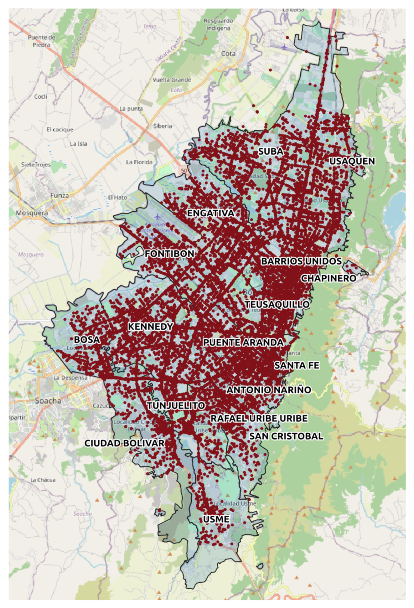
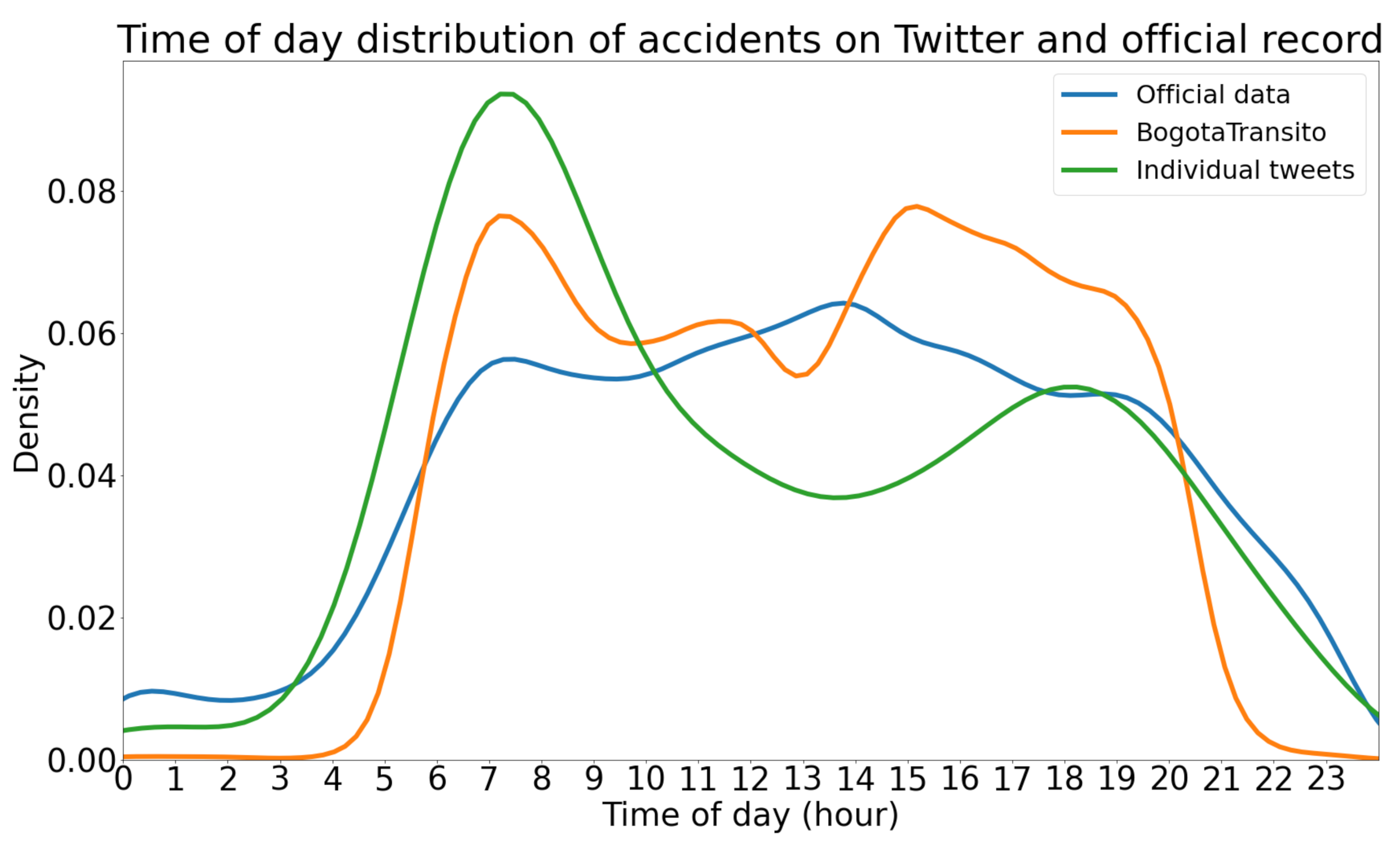
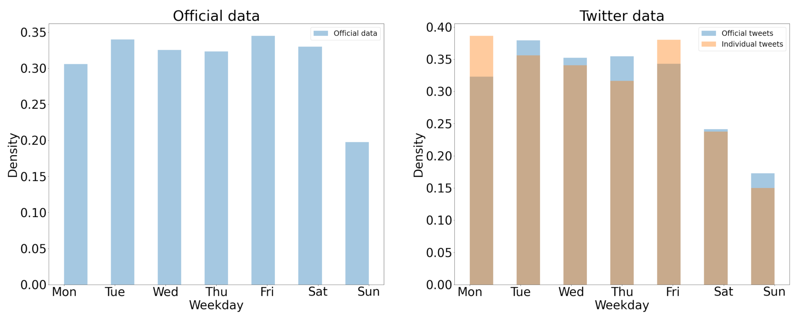
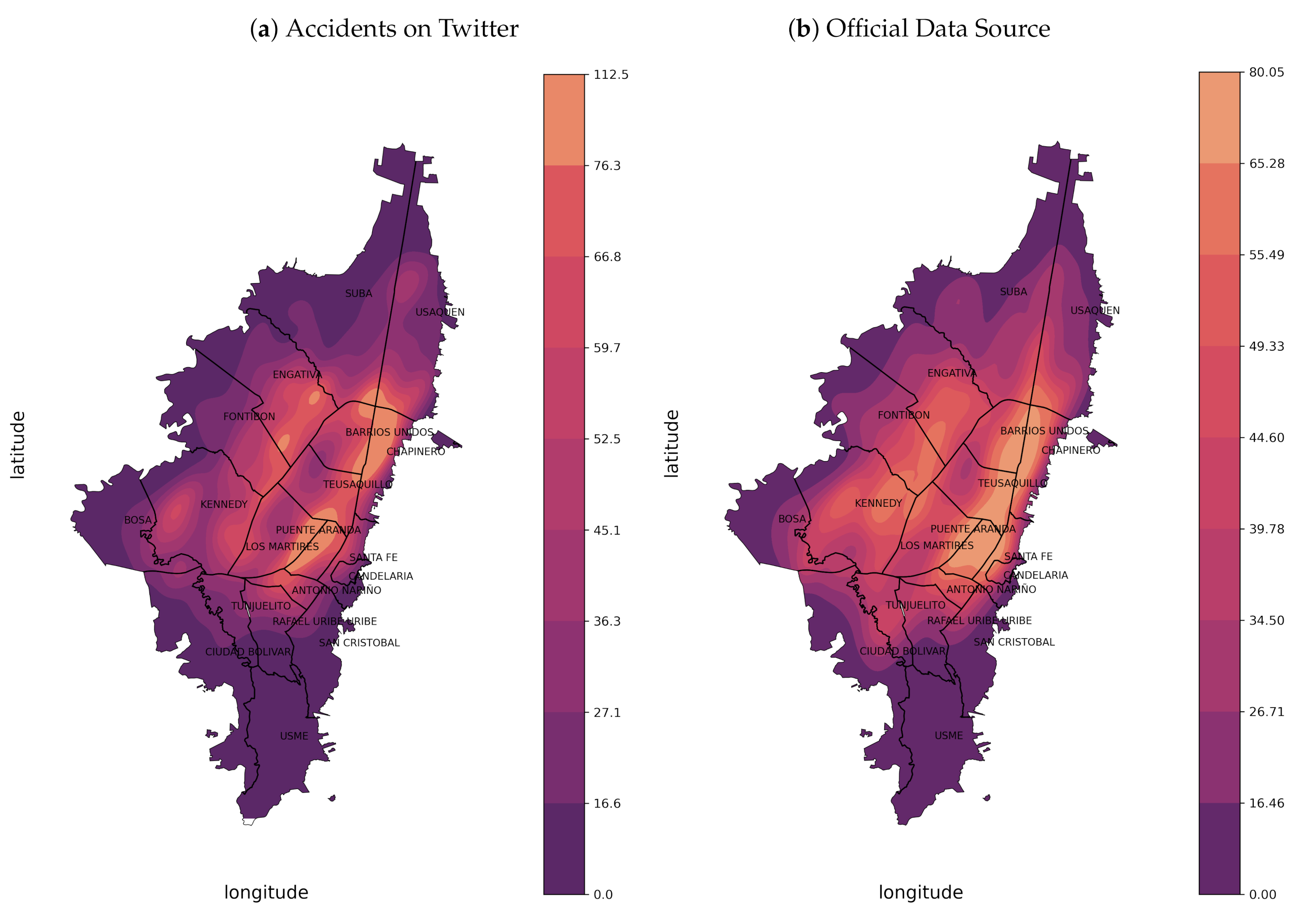
4.5.2. Analysis of the Accident Pattern in Time and Space
5. Discussion and Conclusions
Author Contributions
Funding
Institutional Review Board Statement
Informed Consent Statement
Data Availability Statement
Acknowledgments
Conflicts of Interest
References
- Cookson, G.; Pishue, B. INRIX Global Traffic Scorecard; Number February; INRIX Research: Kirkland, WA, USA, 2018; p. 44. [Google Scholar]
- Víctimas Fallecidas y Lesionadas Valoradas por INMLCF. Nacionales. Agencia Nacional de Seguridad Vial. 2017. Available online: http://ansv.gov.co/observatorio/?op=Contenidos&sec=63&page=20 (accessed on 20 November 2021).
- Wang, S.; He, L.; Stenneth, L.; Yu, P.S.; Li, Z. Citywide traffic congestion estimation with social media. In Proceedings of the 23rd SIGSPATIAL International Conference on Advances in Geographic Information Systems—GIS ’15, Bellevue, WA, USA, 3–6 November 2015; pp. 1–10. [Google Scholar] [CrossRef]
- Fan, X.; He, B.; Wang, C.; Li, J.; Cheng, M.; Huang, H.; Liu, X. Big Data Analytics and Visualization with Spatio-Temporal Correlations for Traffic Accidents. In Proceedings of the 15th International Conference on Algorithms and Architectures for Parallel Processing (ICA3PP 2015), Zhangjiajie, China, 18–20 November 2015; Volume 9531, pp. 255–268. [Google Scholar] [CrossRef]
- Subaweh, M.B.; Wibowo, E.P. Implementation of Pixel Based Adaptive Segmenter method for tracking and counting vehicles in visual surveillance. In Proceedings of the 2016 International Conference on Informatics and Computing (ICIC 2016), Mataram, Indonesia, 28–29 October 2016; pp. 1–5. [Google Scholar] [CrossRef]
- Li, L.; Zhang, J.; Zheng, Y.; Ran, B. Real-Time Traffic Incident Detection with Classification Methods. In Green Intelligent Transportation Systems, Lecture Notes in Electrical Engineering; Springer: Singapore, 2018; Volume 419, pp. 777–788. [Google Scholar] [CrossRef]
- Zhang, S.; Wu, G.; Costeira, J.P.; Moura, J.M. FCN-rLSTM: Deep Spatio-Temporal Neural Networks for Vehicle Counting in City Cameras. In Proceedings of the IEEE International Conference on Computer Vision, Venice, Italy, 22–29 October 2017; pp. 3687–3696. [Google Scholar] [CrossRef]
- Krausz, N.; Lovas, T.; Barsi, Á. Radio frequency identification in supporting traffic safety. Period. Polytech. Civ. Eng. 2017, 61, 727–731. [Google Scholar] [CrossRef][Green Version]
- Wang, S.; Zhang, X.; Cao, J.; He, L.; Stenneth, L.; Yu, P.S.; Li, Z.; Huang, Z. Computing Urban Traffic Congestions by Incorporating Sparse GPS Probe Data and Social Media Data. ACM Trans. Inf. Syst. 2017, 35, 1–30. [Google Scholar] [CrossRef]
- Kuflik, T.; Minkov, E.; Nocera, S.; Grant-Muller, S.; Gal-Tzur, A.; Shoor, I. Automating a framework to extract and analyse transport related social media content: The potential and the challenges. Transp. Res. Part C Emerg. Technol. 2017, 77, 275–291. [Google Scholar] [CrossRef]
- Gu, Y.; Qian, Z.S.; Chen, F. From Twitter to detector: Real-time traffic incident detection using social media data. Transp. Res. Part C Emerg. Technol. 2016, 67, 321–342. [Google Scholar] [CrossRef]
- Arias, B.; Orellana, G.; Orellana, M.; Acosta, M.I. A Text Mining Approach to Discover Real-Time Transit Events from Twitter; Springer International Publishing: Cham, Switzerland, 2019; Volume 884, pp. 266–280. [Google Scholar] [CrossRef]
- Zhang, Z.; He, Q.; Gao, J.; Ni, M. A deep learning approach for detecting traffic accidents from social media data. Transp. Res. Part C Emerg. Technol. 2018, 86, 580–596. [Google Scholar] [CrossRef]
- Sherif, H.M.; Shedid, M.; Senbel, S.A. Real Time Traffic Accident Detection System using Wireless Sensor Network. In Proceedings of the 2014 6th International Conference of Soft Computing and Pattern Recognition (SoCPaR), Tunis, Tunisia, 11–14 August 2014; pp. 59–64. [Google Scholar] [CrossRef]
- Aslam, J.; Lim, S.; Pan, X.; Rus, D. City-scale traffic estimation from a roving sensor network. In SenSys 2012—Proceedings of the 10th ACM Conference on Embedded Networked Sensor Systems; Association for Computing Machinery: New York, NY, USA, 2012; pp. 141–154. [Google Scholar] [CrossRef]
- Zuo, W.; Guo, C.; Liu, J.; Peng, X.; Yang, M. A police and insurance joint management system based on high precision BDS/GPS positioning. Sensors 2018, 18, 169. [Google Scholar] [CrossRef] [PubMed]
- Kwak, H.c.; Kho, S. Predicting crash risk and identifying crash precursors on Korean expressways using loop detector data. Accid. Anal. Prev. 2016, 88, 9–19. [Google Scholar] [CrossRef] [PubMed]
- Li, Z.; Cha, S.K.; Wan, C.; Cui, B.; Zhang, N.; Xu, J. Detecting Anomaly in Traffic Flow from Road Similarity Analysis. In 17th International Conference, WAIM 2016, Proceedings, Part II; Cui, B., Zhang, N., Xu, J., Lian, X., Liu, D., Eds.; Lecture Notes in Computer Science; Springer International Publishing: Cham, Switzerland, 2016; Volume 9659, pp. V–VI. [Google Scholar] [CrossRef]
- Chen, Q.; Song, X.; Yamada, H.; Shibasaki, R. Learning Deep Representation from Big and Heterogeneous Data for Traffic Accident Inference. In Proceedings of the 30th AAAI Conference on Artificial Intelligence (AAAI-16), Phoenix, AZ, USA, 12–17 February 2016; pp. 338–344. [Google Scholar]
- Petalas, Y.G.; Ammari, A.; Georgakis, P.; Nwagboso, C. A Big Data Architecture for Traffic Forecasting Using Multi-Source Information; ALGOCLOUD 2016; Springer International Publishing: Cham, Switzerland, 2017; Volume 10230, pp. 65–83. [Google Scholar] [CrossRef]
- Salas, A.; Georgakis, P.; Nwagboso, C.; Ammari, A.; Petalas, I. Traffic Event Detection Framework Using Social Media. In Proceedings of the IEEE International Conference on Smart Grid and Smart Cities, Singapore, 23–26 July 2017; p. 5. [Google Scholar] [CrossRef]
- Salas, A.; Georgakis, P.; Petalas, Y. Incident Detection Using Data from Social Media. In Proceedings of the 2017 IEEE 20th International Conference on Intelligent Transportation Systems (ITSC), Yokohama, Japan, 16–19 October 2017; pp. 751–755. [Google Scholar] [CrossRef]
- Kurniawan, D.A.; Wibirama, S.; Setiawan, N.A. Real-time traffic classification with Twitter data mining. In Proceedings of the 2016 8th International Conference on Information Technology and Electrical Engineering (ICITEE), Yogyakarta, Indonesia, 5–6 October 2016; pp. 1–5. [Google Scholar] [CrossRef]
- Pereira, J.; Pasquali, A.; Saleiro, P.; Rossetti, R. Transportation in Social Media: An Automatic Classifier for Travel-Related Tweets. In Proceedings of the 18th EPIA Conference on Artificial Intelligence (EPIA 2017), Porto, Portugal, 5–8 September 2017; Volume 8154, pp. 355–366. [Google Scholar] [CrossRef]
- Nguyen, H.; Liu, W.; Rivera, P.; Chen, F. TrafficWatch: Real-Time Traffic Incident Detection and Monitoring Using Social Media Hoang. In PAKDD: Pacific-Asia Conference on Knowledge Discovery and Data Mining; Bailey, J., Khan, L., Washio, T., Dobbie, G., Huang, J.Z., Wang, R., Eds.; Lecture Notes in Computer Science; Springer International Publishing: Cham, Switzerland, 2016; Volume 9651, pp. 540–551. [Google Scholar] [CrossRef]
- Schulz, A.; Ristoski, P.; Paulheim, H. I see a car crash: Real-time detection of small scale incidents in microblogs. In The Semantic Web: ESWC 2013 Satellite Events. ESWC 2013. Lecture Notes in Computer Science; Springer: Berlin/Heidelberg, Germany, 2013; pp. 22–33. [Google Scholar] [CrossRef]
- Caimmi, B.; Vallejos, S.; Berdun, L.; Soria, Ï.; Amandi, A.; Campo, M. Detección de incidentes de tránsito en Twitter. In Proceedings of the 2016 IEEE Biennial Congress of Argentina (ARGENCON 2016), Buenos Aires, Argentina, 15–17 June 2016; pp. 1–6. [Google Scholar] [CrossRef]
- Gutiérrez, C.; Figueiras, P.; Oliveira, P.; Costa, R.; Jardim-goncalves, R. An Approach for Detecting Traffic Events Using Social Media. In Emerging Trends and Advanced Technologies for Computational Intelligence; Springer: Cham, Switzerland, 2016; Volume 647. [Google Scholar] [CrossRef]
- Anantharam, P.; Barnaghi, P.; Thirunarayan, K.; Sheth, A. Extracting City Traffic Events from Social Streams. ACM Trans. Intell. Syst. Technol. 2015, 6, 1–27. [Google Scholar] [CrossRef]
- Chen, Y.; Lv, Y.; Wang, X.; Wang, F.Y. A convolutional neural network for traffic information sensing from social media text. In Proceedings of the IEEE Conference on Intelligent Transportation Systems (ITSC), Yokohama, Japan, 16–19 October 2017; pp. 1–6. [Google Scholar] [CrossRef]
- Peres, R.; Esteves, D.; Maheshwari, G. Bidirectional LSTM with a Context Input Window for Named Entity Recognition in Tweets. In Proceedings of the K-CAP 2017: Knowledge Capture Conference (K-CAP 2017), New York, NY, USA, 4–6 December 2017; pp. 1–4. [Google Scholar] [CrossRef]
- Aguilar, G.; López Monroy, A.P.; González, F.; Solorio, T. Modeling Noisiness to Recognize Named Entities using Multitask Neural Networks on Social Media. In Proceedings of the NAACL-HLT 2018 Association for Computational Linguistics, New Orleans, LA, USA, 1–6 June 2018; Volume 1, pp. 1401–1412. [Google Scholar] [CrossRef]
- Gelernter, J.; Balaji, S. An algorithm for local geoparsing of microtext. GeoInformatica 2013, 17, 635–667. [Google Scholar] [CrossRef]
- Ritter, A.; Clark, S.; Mausam; Etzioni, O. Named entity recognition in tweets: An experimental study. In Proceedings of the Conference on Empirical Methods in Natural Language Processing, Edinburgh, UK, 27–32 July 2011; pp. 1524–1534. [Google Scholar]
- Malmasi, S.; Dras, M. Location Mention Detection in Tweets and Microblogs. In PACLING 2015, CCIS; Oxford University Press: Oxford, UK, 2016; pp. 123–134. [Google Scholar] [CrossRef]
- Gelernter, J.; Zhang, W. Cross-lingual geo-parsing for non-structured data. In Proceedings of the 7th Workshop on Geographic Information Retrieval, Association for Computing Machinery, New York, NY, USA, 5 November 2013; pp. 64–71. [Google Scholar] [CrossRef]
- Sagcan, M.; Karagoz, P. Toponym Recognition in Social Media for Estimating the Location of Events. In Proceedings of the 2015 IEEE International Conference on Data Mining Workshop (ICDMW), Atlantic City, NJ, USA, 14–17 November 2015; pp. 33–39. [Google Scholar] [CrossRef]
- Le, Q.; Mikolov, T. Distributed Representations of Sentences and Documents. In Proceedings of the 31st International Conference on Machine Learning, Beijing, China, 21–26 June 2014; Volume 32. [Google Scholar]
- Okur, E.; Demir, H.; Özgür, A. Named entity recognition on twitter for Turkish using semi-supervised learning with word embeddings. In Proceedings of the 10th International Conference on Language Resources and Evaluation (LREC 2016), Portoroz, Slovenia, 23–28 May 2016; pp. 549–555. [Google Scholar]
- Mikolov, T.; Chen, K.; Corrado, G.; Dean, J. Efficient estimation of word representations in vector space. In Proceedings of the 1st International Conference on Learning Representations, ICLR 2013—Workshop Track Proceedings, Scottsdale, AZ, USA, 2–4 May 2013; pp. 1–12. [Google Scholar]
- Devlin, J.; Chang, M.W.; Lee, K.; Toutanova, K. BERT: Pre-training of Deep Bidirectional Transformers for Language Understanding. In Proceedings of the 2019 Conference of the North American Chapter of the Association for Computational Linguistics: Human Language Technologies, Minneapolis, MN, USA, 2–7 June 2019. [Google Scholar]
- Cañete, J.; Chaperon, G.; Fuentes, R.; Pérez, J. Spanish Pre-Trained BERT Model and Evaluation Data. In Proceedings of the PML4DC at ICLR 2020, Addis Ababa, Ethiopia, 26 April 2020; pp. 1–10. [Google Scholar]
- Norvig, P. Natural Language Corpus Data. In Beautiful Data: The Stories Behind Elegant Data Solutions; O’Reilly Media, Inc.: Sebastopol, CA, USA, 2009; pp. 219–242. ISBN 978-0596157111. [Google Scholar]
- Honnibal, M.; Johnson, M. An improved non-monotonic transition system for dependency parsing. In Proceedings of the Conference Proceedings—EMNLP 2015: Conference on Empirical Methods in Natural Language Processing, Lisbon, Portugal, 17–21 September 2015; pp. 1373–1378. [Google Scholar] [CrossRef]
- Taufik, N.; Wicaksono, A.F.; Adriani, M. Named entity recognition on Indonesian microblog messages. In Proceedings of the 2016 International Conference on Asian Language Processing (IALP 2016), Tainan, Taiwan, 21–23 November 2016; pp. 358–361. [Google Scholar] [CrossRef]
- García-Pablos, A.; Perez, N.; Cuadros, M. Sensitive Data Detection and Classification in Spanish Clinical Text: Experiments with BERT. In Proceedings of the 12th Edition of Language Resources and Evaluation Conference (LREC2020), Marseille, France, 11–16 May 2019; Available online: http://www.lrec-conf.org/proceedings/lrec2020/pdf/2020.lrec-1.552.pdf (accessed on 20 November 2021).


| Twitter Usernames | |||
|---|---|---|---|
| @BogotaTransito | @Citytv | @RedapBogota | @WazeTrafficBog |
| @CIVICOSBOG | @rutassitp | @SectorMovilidad | @UMVbogota |
| @idubogota | @transmilenio | @IDIGER | |
| Search Equations |
|---|
| (“accidente” OR “choque” OR “incidente vial” OR “incidente” OR “choque entre” ) -RT -“plan de choque” |
| (“atropello” OR “tráfico” OR “trafico” OR “tránsito” OR “transito” OR “#trafico” OR “#traficobogota” OR “sitp” OR “transmilenio”) -RT |
| #hashtag or @username | Results |
|---|---|
| #puentearanda | puente aranda |
| #avenida68 | avenida 68 |
| @CorferiasBogota | corferias bogota |
| Collection Filter | # Collected Tweets |
|---|---|
| Stream Bogotá | 4,027,313 |
| Stream Follow/Timeline User | 574,816 |
| Search Token | 271,153 |
| Search Timeline User | 100,618 |
| Tweets | Description |
|---|---|
| Hueco causa accidentalidad Cra. 68c #10-16 sur, Bogotá | Accident |
| Justo ahora 1:22 p.m. en 21 angeles Av Suba gratamira (calle 145 Av Suba) complicaciones viales por accidente @BogotaTransito @ALCALDIASUBA11 @SectorMovilidad | Accident |
| Semáforos de la Carrera 24 con Calle 9 en amarillo intermitente, Tanto por la calle como por la carrera con riesgo de incidente vehicular | No Accident |
| Incidente vial entre bus y un motociclista en la calle 86a con carrera 111a. Unidad de @TransitoBta y asignadas. | @BogotaTransito |
| Two different reports in the same tweet |
| #ArribaBogotá Por culpa de este hueco en la calle 27sur, una mujer sufrió un grave accidente de tránsito. | Vague location |
| B-Loc | I-Loc | B-Time | I-Time | O | |
|---|---|---|---|---|---|
| Trainset | 1462 | 3768 | 131 | 112 | 20,242 |
| Testset | 369 | 893 | 33 | 33 | 5038 |
| Total | 1831 | 4661 | 164 | 145 | 25,280 |
| Preprocessing | Embedding | Acc (%) | F1 (%) | R (%) | P (%) |
|---|---|---|---|---|---|
| Lemma | Doc2vec (*our) | 96.85 | 96.85 | 96.85 | 96.85 |
| TF IDF | 96.69 | 96.69 | 96.69 | 96.71 | |
| Lemma + Stopwords | Doc2vec | 96.63 | 96.63 | 96.63 | 96.65 |
| TF IDF | 96.19 | 96.19 | 96.20 | 96.22 | |
| Stem | Doc2vec | 96.14 | 96.14 | 96.14 | 96.16 |
| TF IDF | 96.69 | 96.69 | 96.69 | 96.71 | |
| Stem + Stopwords | Doc2vec | 96.84 | 96.84 | 96.84 | 96.86 |
| TF IDF | 96.03 | 96.03 | 96.04 | 96.05 | |
| Cleaning steps for BERT | BERT | 95.37 | 95.37 | 95.37 | 95.40 |
| Pipeline Model | Acc (%) | F1 (%) | R (%) | P (%) |
|---|---|---|---|---|
| doc2vec + lemma + SVM (*our) | 96.85 | 96.85 | 96.85 | 96.85 |
| TF IDF + stem + NB | 93.40 | 93.40 | 93.40 | 93.45 |
| TF IDF + lemma + RF | 96.08 | 96.08 | 96.08 | 96.11 |
| TF IDF + stem + NN | 96.22 | 96.12 | 95.17 | 97.09 |
| Model | F1 (%) | Recall (%) | Precision (%) |
|---|---|---|---|
| CRF | 91.66 | 89.76 | 93.80 |
| BiLSTM | 90.88 | 89.77 | 92.25 |
| BiLSTM + CRF | 84.22 | 81.55 | 88.50 |
| SpaCy | 91.97 | 91.97 | 92.17 |
| Best Model | # Entities | F1 (%) | Recall (%) | Precision (%) |
|---|---|---|---|---|
| B-loc | 369 | 88.70 | 87.82 | 89.60 |
| I-loc | 893 | 94.83 | 95.82 | 93.86 |
| B-time | 33 | 62.22 | 51.85 | 77.78 |
| I-time | 33 | 74.51 | 65.52 | 86.36 |
| Overall | 1328 | 91.97 | 91.97 | 92.17 |
| Author | Language | Region | Classifier | Class | F1 (%) |
|---|---|---|---|---|---|
| Our approach | Spanish | Bogotá, Colombia | Do2vec + SVM | Accident Incident | 96.85 |
| Arias et al. [12] | Spanish | Cuenca, Ecuador | BoW + SVM | Traffic Incident | 85.10 |
| Caimmi et al. [27] | Spanish | Buenos Aires, Argentina | TF IDF + Ensemble SVM, SMO, NB | Traffic Incident | 91.44 |
| Pereira et al. [24] | Portuguese | Brasil | BoW + word2vec + SVM | Travel-Related | 85.48 |
| Author | Language | Region | NER | Classes | F1 (%) |
|---|---|---|---|---|---|
| Our approach | Spanish | Bogotá, Colombia | Spacy retrained with tweets | Loc, Time | 91.97 |
| Arias et al. [12] | Spanish | Cuenca, Ecuador | Rule-Based | Loc | 80.61 |
| Gelernter & Zhang [36] | Spanish | Spanish Tweets | Rule-Based + NER Software + Translate | Toponymy | 86.10 |
| Sagcan & Karagoz [37] | Turkish | Turkish Tweets | Rule-Based + CRF | Loc | 62.00 |
| Collection Filter | Non-Accidents | Accidents | Tweets Location | ||
|---|---|---|---|---|---|
| # | % | # | % | ||
| Stream Bogotá | 4,021,481 | 99.85 | 5832 | 0.15 | 4463 |
| Stream Follow/Timeline User | 487,545 | 84.8 | 87,271 | 15.2 | 80,277 |
| Search Token | 210,183 | 77.5 | 60,970 | 22.5 | 54,765 |
| Search Timeline User | 50,507 | 50.2 | 50,111 | 49.8 | 47,398 |
| Tweet | Label Prediction |
|---|---|
| Semáforos de la Carrera 24 con Calle 9 en amarillo intermitente, Tanto por la calle como por la carrera con riesgo de incidente vehicular | No accident |
| Inicia marcha SENA Kra 30A esta hora inicia desplazamiento de estudiantes del SENA sede carrera 30 con calle 14 por toda la Av. NQS hacia el norte, utilizando calzada mixta con afectación de calzada de TransMilenio. | No accident |
| Hueco causa accidentalidad Cra. 68c #10-16 sur, Bogotá | Accident |
| A esta hora nuestras unidades brindan apoyo en la Av primero de mayo por 24, donde se presenta un choque entre un vehículo particular y una motocicleta. | Accident |
| Month | # Tweets TA | # Tweets Coordinates |
|---|---|---|
| October | 3682 | 2194 |
| November | 4072 | 2358 |
| December | 3634 | 2114 |
| January | 4316 | 2692 |
| February | 4127 | 2534 |
| Marh | 4029 | 2500 |
| April | 3697 | 2241 |
| May | 4123 | 2545 |
| June | 5281 | 3287 |
| July | 6274 | 3897 |
| Total | 43,235 | 26,362 |
| Data Source | Number of Reports | |
|---|---|---|
| Official data | 25,299 | |
| All reports | Excluding @BogotaTransito | |
| Twitter data | 26,362 | 1431 |
| Twitter (matched by Official data in 1 km and 2 h) | 8619 | 455 |
| # Twitter “additional” reports | 17,743 | 976 |
| Tweet | Time Difference |
|---|---|
| Calle 55 sur carrera 19B Choque con herido ya hay Ambulancia se necesita @TransitoPolicia @BogotaTransito @SectorMovilidad @TransitoBta | 23 s later |
| Aparatoso accidente en la Av. Córdoba con calle 127 sentido sur-norte. Trancón, se recomienda usar vías alternas. @gusgomez1701 @CaracolRadio @SectorMovilidad | 58 min later |
| Incidente vial entre dos particulares en la Calle 19 con Carrera 34, sentido occidente-oriente. Unidad de @TransitoBta asignada. | 1 h 37 min later by BogotaTransito |
| @BogotaTransito buenos días, necesitamos su ayuda en la carrera 7 con calle 163, choque de sitp con taxi. | 2 min earlier |
| @TransMilenio @PoliciaBogota Peatón atropellado en troncal calle 80, estación Av 68, Se requiere ambulancia urgente!!!!! | 15 min earlier |
Publisher’s Note: MDPI stays neutral with regard to jurisdictional claims in published maps and institutional affiliations. |
© 2022 by the authors. Licensee MDPI, Basel, Switzerland. This article is an open access article distributed under the terms and conditions of the Creative Commons Attribution (CC BY) license (https://creativecommons.org/licenses/by/4.0/).
Share and Cite
Suat-Rojas, N.; Gutierrez-Osorio, C.; Pedraza, C. Extraction and Analysis of Social Networks Data to Detect Traffic Accidents. Information 2022, 13, 26. https://doi.org/10.3390/info13010026
Suat-Rojas N, Gutierrez-Osorio C, Pedraza C. Extraction and Analysis of Social Networks Data to Detect Traffic Accidents. Information. 2022; 13(1):26. https://doi.org/10.3390/info13010026
Chicago/Turabian StyleSuat-Rojas, Nestor, Camilo Gutierrez-Osorio, and Cesar Pedraza. 2022. "Extraction and Analysis of Social Networks Data to Detect Traffic Accidents" Information 13, no. 1: 26. https://doi.org/10.3390/info13010026
APA StyleSuat-Rojas, N., Gutierrez-Osorio, C., & Pedraza, C. (2022). Extraction and Analysis of Social Networks Data to Detect Traffic Accidents. Information, 13(1), 26. https://doi.org/10.3390/info13010026