Article

Fast, Efficient and Flexible Particle Accelerator Optimisation Using Densely Connected and Invertible Neural Networks

Paul Scherrer Institut, 5232 Villigen, Switzerland
*
Author to whom correspondence should be addressed.
Information 2021, 12(9), 351; https://doi.org/10.3390/info12090351
Submission received: 16 July 2021 / Revised: 25 August 2021 / Accepted: 26 August 2021 / Published: 28 August 2021
(This article belongs to the Special Issue Machine Learning and Accelerator Technology)

Abstract

:
Particle accelerators are enabling tools for scientific exploration and discovery in various disciplines. However, finding optimised operation points for these complex machines is a challenging task due to the large number of parameters involved and the underlying non-linear dynamics. Here, we introduce two families of data-driven surrogate models, based on deep and invertible neural networks, that can replace the expensive physics computer models. These models are employed in multi-objective optimisations to find Pareto optimal operation points for two fundamentally different types of particle accelerators. Our approach reduces the time-to-solution for a multi-objective accelerator optimisation up to a factor of 640 and the computational cost up to 98%. The framework established here should pave the way for future online and real-time multi-objective optimisation of particle accelerators.

1. Introduction

Advances in accelerator science and technology have enabled discoveries in particle physics and other fields—from chemistry and biology to medical applications—for more than a century [1], with no end in sight [2]. Particle accelerators consist of a multitude of building blocks, and the relationship between changes in machine settings, known as design variables, and the corresponding particle-beam response is often non-linear. For this reason, the development and operation of a particle accelerator rely heavily on computational models. These models use first principles of physics to state the equations of motion, while numerical algorithms are then employed to solve them. These models provide valuable insight, but their high computational cost is prohibitive for many applications. For example, a single simulation of the Argonne Wakefield Accelerator (AWA) (Figure 1) takes approximately ten minutes with the high-fidelity physics model Object-Oriented Parallel Accelerator Library (OPAL) [3], which renders such models unsuitable for real-time usage. In order to achieve optimal operation points of these machines, genetic algorithms (GAs) are typically the method of choice for solving multi-objective optimisation problems [4,5,6,7,8]. However, an optimisation sometimes requires thousands of model evaluations. For this reason, the time-to-solution can easily be in the order of days. Recent work [9] addressed this issue by training a data-driven surrogate model to approximate the computer model at a single position of interest. Evaluating such a surrogate model takes less than a second and results in predictions that are very close to the high-fidelity physics model.
Related to these works, Scheinker et al. developed and demonstrated an online multi-timescale multi-objective optimisation algorithm that performs real-time feedback on particle accelerators [10]. In contrast to our contribution, they demonstrate a general control theoretical motivated feedback algorithm, capable of performing online multi-objective optimisation. Bayesian optimisation in combination with particle-in-cell simulations [11] is used to tune a plasma accelerator autonomously to the beam energy spread to the sub-percent at a given energy and intensity.
In this work, we introduce two new surrogate models, a forward model and an invertible model. Both are designed to model the machine at any longitudinal position, overcoming a main limitation of existing approaches. Moreover, the proposed methods for building these models are general enough to be applicable to any kind of particle accelerators. We demonstrate the generality of the ansatz by considering a linear accelerator and a quasi-circular machine, i.e., a cyclotron. Furthermore, the fast surrogate models enable optimisations on time scales suitable for online and real-time multi-objective optimisations of particle accelerators.
The forward model resembles existing models described, e.g., in [9]. While previous work focused on approximating OPAL only at one position (usually at the end) of the accelerator (as in [9]), our new model provides an approximation to OPAL at a multitude of positions along the accelerator, allowing us to estimate beam properties along the entire accelerator depicted in Figure 1d. To achieve this goal, our model takes both the design variables and the position along the accelerator as input and predicts the beam properties at that position. Consequently, our model is a complete replacement for OPAL and does not limit our options of objectives and constraints for beam optimisations. Existing models are not capable of optimising the beam properties at multiple positions at the same time, but our forward model enables such sophisticated optimisations, which we demonstrate empirically.
The invertible model is capable of solving both the forward and the inverse problem by providing two kinds of predictions, called the forward and the inverse prediction. The forward prediction approximates OPAL, i.e., it calculates the beam properties corresponding to a given machine configuration. The inverse prediction takes a user-imposed target beam and returns a machine configuration that realises an approximation to such a beam. In order to incorporate expert intuition and knowledge in the optimisation, the result of the inverse prediction initialises a GA-based multi-objective optimisation, which then requires fewer generations to converge than when the usual random initialisation is used.
We demonstrate the capabilities of the two surrogate models with the two real-world examples depicted in Figure 1. The first example is the AWA, which is a linear accelerator. The second one is the cyclotron used for the proposed Isotope Decay-at-Rest experiment, a proposed very-high-intensity electron-antineutrino source (from here on called the IsoDAR machine). We developed a forward model and an invertible model for both of these fundamentally different accelerators. Furthermore, we used them for a multi-objective accelerator optimisation to find machine configurations for desired beam properties.

1.1. Physics Models and Datasets

For both accelerators we used the same underlying physics model, based on the OPAL accelerator simulation framework. The dynamics of an accelerator are given by the following function:
f : R m × R R n f ( x , s ) = y ( s ) ,
where the quantity x represents a vector of machine settings (design variables), the scalar s R denotes the position along the accelerator and the vector y ( s ) R n denotes the beam properties (quantities of interest). The function f represents the OPAL high-fidelity physics model.
Our surrogate models learn the relationship between design variables and quantities of interest based on examples, which means that we need to incorporate the physics of an accelerator into a dataset. We achieve this by sampling the space of design variables randomly and evaluating the sampled configurations of interest at multiple positions along the machine. One sample in the dataset consists of the design variables, a position along the machine and the corresponding quantities of interest.

1.2. Specifics of the Argonne Wakefield Accelerator Model

The AWA accelerator [12] consists mainly of an electron gun, several radio-frequency cavities for accelerating the electrons and magnets for keeping the beam focused. The electron gun generates bunches that form a train of Gaussians in the longitudinal direction, separated by a peak-to-peak distance λ . Other electron-gun variables are the gun phase ϕ , the charge Q, the laser spot size (SIGXY) and the current in the buck focusing and matching solenoids (BFS and MS). For details, we refer to Figure 1d. In total, we have nine design variables, denoted x R 9 , that define the various operation points of the AWA. The ranges of x are determined by the physical limitations of the accelerator and listed in Table A3. The quantities of interest (QoIs), y R 8 are as follows: the transversal root-mean-square beam sizes σ x , σ y , the transversal normalised emittances ϵ x , ϵ y , the mean bunch energy E, the energy spread of the beam Δ E and the correlations between transversal position and momentum Corr ( x , p x ) , Corr ( y , p y ) . A summary and more details about the used QoIs are given in Table A2.
We built a labeled dataset of the AWA by using OPAL and the latin hypercube procedure [13] in order to sample the search space of x, which results in a training/validation set of 18,065 points and a test set of 913 points.

1.3. Specifics of the IsoDAR Cyclotron Model

The simulations are based on the latest IsoDAR [14,15,16] cyclotron design, with the nominal beam intensity of 5 mA H 2 + beam (equivalent to 10 mA of protons). Ongoing modeling efforts of IsoDAR consider the radial momenta p r 0 , the injection radius r 0 , the phase ϕ r f of the radio frequency of the acceleration cavities and the root mean square beam sizes σ x , σ y , σ z at injection. The physical ranges of the machine settings are given in Table A4. The surrogate models predict the transversal and longitudinal root mean square beam sizes σ x , σ y , σ z , the projected emittances ϵ x , ϵ y , ϵ z , the beam halo parameters h x , h y , h z , the energy E, the energy spread of the beam Δ E and the particle loss N l (see Table A2). For this example, we have six machine settings x R 6 and twelve quantities of interest y R 12 . All the samples are taken at turn 95, in the vicinity of the extraction channel.
The labeled dataset, obtained with OPAL, consists of 5000 random machine configurations. Among these, 1000 samples are randomly selected and used as the test set, 800 for the validation set and the remaining 3200 samples form the training set.

2. Results

2.1. Forward and Invertible Models

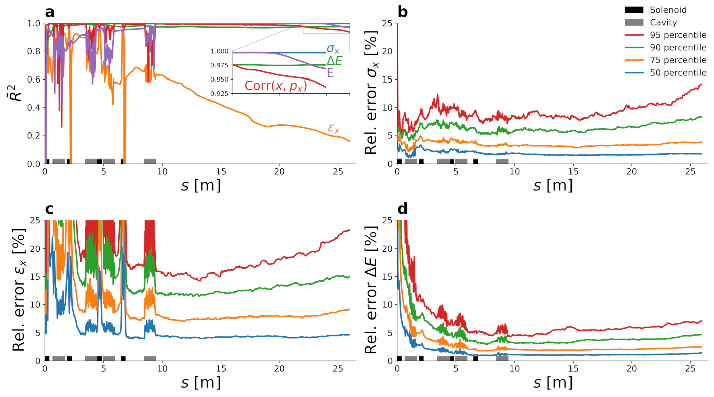
We assess the quality of the surrogate models by evaluating the adjusted coefficient of determination ( R ¯ 2 ) and the relative prediction error at 95% confidence on the test set; i.e., data that have not been used during the development of the models. For the AWA model, the R ¯ 2 values for the forward model are very close to one at nearly all positions along the machine, except for the solenoids and cavities. As a consequence, the variance of the dataset is explained well, as can be observed in Figure 2a. Due to the presence of angular momenta inside the solenoid region, the variance of the emittance is not captured well. In OPAL this effect is not suppressed, however, Bush’s theorem assures that, at the exit, the effect is reversed and does not contribute to our quantities of interest. In consequence, only the variance of the emittance is not captured well inside the solenoids and cavities, respectively. However, the relative prediction error for this quantity is still less than 25% for 95% confidence, as depicted in Figure 2c. The relative errors for the other quantities are even lower than 15% and 10% for σ x (Figure 2b) and Δ E (Figure 2d), respectively.
For the forward surrogate model of IsoDAR, the variance of the dataset is captured very well with a minimum R ¯ 2 value of 0.95 among all predicted values, except for the quantities in z-direction. Here, it ranges between 0.82 and 0.86. The relative prediction error of the forward model is at most 5.6%.
Since we are mainly interested in the beam parameters, we evaluated the invertible model by performing first the inversion, computing machine settings from beam parameters, with the invertible model and then a forward prediction with the forward model. For the AWA model the error at 95% confidence is almost 40% for the beam size, emittance and energy spread. Nevertheless, the sampling error is only 20% for three out of four target beams in the test set. The energy, on the other hand, is obtained almost with perfect accuracy.
For the IsoDAR model, the relative errors for 95% confidence range from 0.08% to 11%. The corresponding R ¯ 2 values lie between 0.79 and 0.96 except for the longitudinal quantities, for which we obtained values between 0.65 and 0.77. The detailed values for the IsoDAR model can be found in Table A1, Figure A1 and Figure A2.
Further details about the datasets and the model parameters can be found in Appendix B and Appendix C.

2.2. Multi-Objective Optimisation

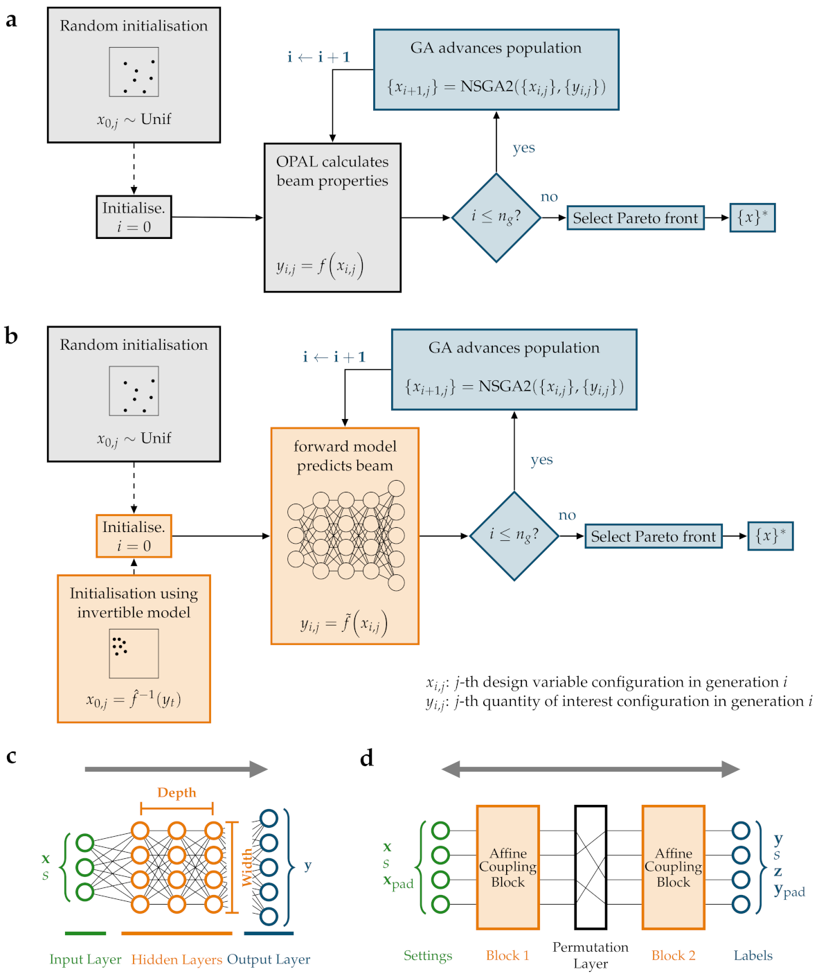
To find good operation points for the accelerators, we solved multi-objective optimisation problems [5,6,9,17]. The standard approach for that is visualized in Figure 3a: A physics based model, such as OPAL, together with a GA and random initialization is used. We investigate two other approaches depicted in Figure 3b. First, we use a GA together with the forward model, instead of OPAL, and a random initialisation. In the second approach, the GA and the forward model are still employed, but the invertible model additionally provides us with a good initial guess for the optimisation.

2.3. Performance Metrics for the Optimisations

By characterising an approximation to the Pareto front, the set of optimal solutions encompasses two main aspects. First, we strive to converge quickly, using as few iterations as possible, towards non-dominated quantities of interest. The range of the objectives in the non-dominated set is chosen to analyse the convergence behaviour. Thus, for each generation the ranges of all objectives individually are compared for the two optimisation approaches. Second, we demand that the non-dominated quantities of interest are diverse, i.e., well spread out over the entire approximated Pareto front. The convex hull volume V c h (see Appendix A.1 for more details), the number of solutions of the non-dominated set, as well as the generational distance [18] and the hypervolume difference (i.e., the difference between the hypervolume of the optimal solution and the hypervolumes of the Pareto front of each generation, with a reference point chosen close to the Nadir point [19]) assess this quality aspect. Finally, plotting projections of the non-dominating set provides a holistic view to compare the effect of the initialisation strategies (random vs. invertible model initialisation) on both the convergence and the diversity of the non-dominated set. These plots show the evolution of the solutions of the optimisation problem across the generations directly.

2.4. Multi-Objective Optimisation for AWA

The constrained multi-objective optimisation problem of the following:
min σ x ( 26 m ) min ϵ x ( 26 m ) min Δ E ( 26 m ) s . t . σ x ( s ) 2 mm , s 0 , 0.25 , 0.5 , , 10 m σ x ( s ) 5 mm , s 0 , 0.25 , 0.5 , , 10 m Corr ( x , p x ) 0.1 , at 26 m ,
represents a generic multi-objective optimisation task, found in many of the past and future AWA experiments [12]. The optimisation of beam parameters was required at 26 m for a pilot experiment performed in 2020, regarding a new scheme for electron cooling. In addition, there were multiple constraints at various positions along the accelerator. We solved the optimisation problem twice, once initialising the GA population randomly and once initialising the GA population with the invertible model outcome, where we utilized target values for the beam parameters as listed in Table A6.
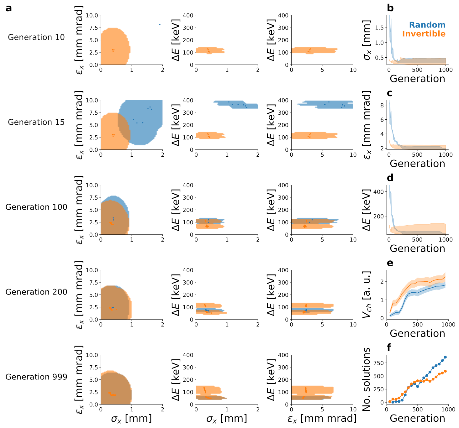
The objective values for different generations are depicted in Figure 4a. The optimisation initialised with the invertible model converged almost entirely after 10 generations. If random initialisation is used, more than 100 generations are needed to arrive at the same optimal configurations. The ranges of the beam properties in the non-dominated set confirm this observation (Figure 4b–d). Using the invertible model results in a bigger hypervolume even when prediction uncertainty is accounted for (Figure 4e). Furthermore, the optimisation initialised with the invertible model finds more solutions during the first 500 generations (Figure 4f). These two statements imply that the initialisation with the invertible model finds both more and more diverse non-dominated design variables.
The non-dominated feasible machine settings are evaluated with OPAL (dots in Figure 5a–c) in order to validate the predicted optimal objective values. All the OPAL evaluated points lie within the region of uncertainty for the optimal objective values at 90% confidence.
In Figure 5d, deeper insights into the constraint on the correlation parameter ( C o r r ( x , P x ) ) is given. Although the surrogate models found many configurations lying outside the allowed region, both initialisation strategies result in at least some feasible configurations. Importantly, no machine configuration in the training/validation set is feasible according to the optimisation problem, that means that no sample in these datasets fulfills the optimisation constraints. Nevertheless, some optimal points fulfill the correlation constraint.

2.5. Multi-Objective Optimisation for IsoDAR

For the IsoDAR case, we solved a two-objective optimisation problem, similar to that introduced by Edelen et al. [9]. We aim to minimise simultaneously the projected emittance ϵ x and the energy spread Δ E of the beam without any constraints.
min Δ E min ϵ x .
As before, the optimisation problem is solved with a GA by using the forward surrogate model. First, a random initialisation is used and then an initialisation using the invertible model with the target beam parameters in Table A5 is performed.
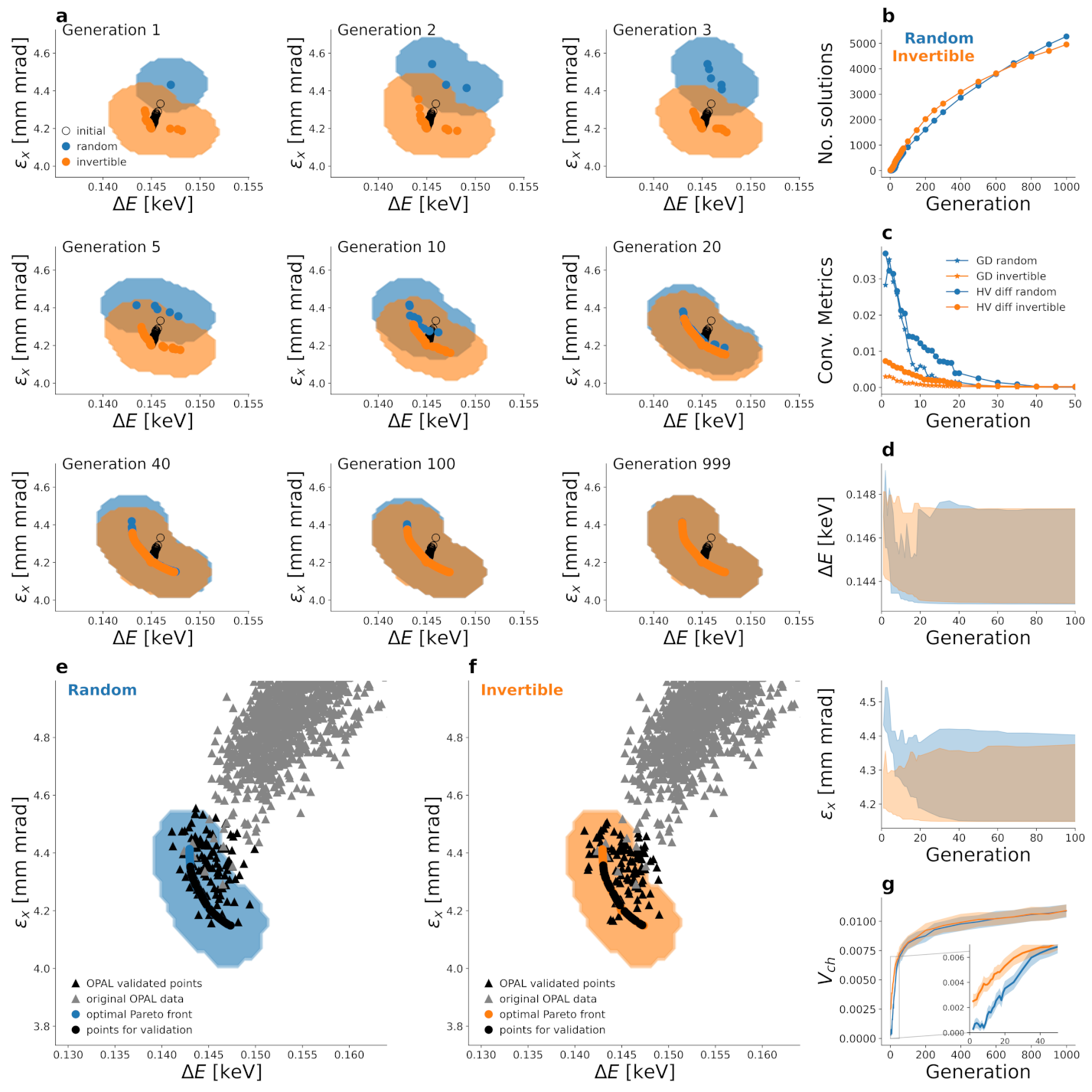
The convergence of the objective values for the two optimisation approaches is depicted in Figure 6a. Both approaches result in the same non-dominated set. The optimisation with the invertible model initialisation converges faster and finds more optimal points already in the first few generations. The random initialisation approach needs approximately 40 generations until it is at the same level. Figure 6b shows that both initialisation schemes result in the end to nearly the same number of solutions. The difference of the objective values for the two approaches in the first generations of the optimisation can also be observed in Figure 6d, which depicts the ranges from minimum to maximum values of the non-dominated set for the two objectives.
The performance-metrics plots Figure 6c,g show the behaviour of the two approaches quantitatively. The generational distance for the invertible model initialisation starts at a much lower value. Therefore, the non-dominated sets found in the first generation are already closer to the final non-dominated set than the ones found with the random initialisation. The lower hypervolume difference and the higher convex hull volume for the invertible model initialisation indicate that the initial non-dominated set is more widely spread, but these advantages vanish after approximately 40 generations.
In order to validate the optimisation results, we randomly chose 100 points of the non-dominated sets of both approaches and simulated them with OPAL. We did not evaluate all non-dominated machine settings because of the high computational cost of OPAL for the IsoDAR example. As can be seen in Figure 6e,f, nearly all of the OPAL points lie within the 90-percent confidence region of the prediction with the test set, although only few points of the original OPAL dataset are in this area.

2.6. Computational Advantages

We compare solving an optimisation problem with OPAL to our approach of using a forward surrogate model instead of OPAL. There are two quantities to be considered for the speedup analysis. First, the time-to-solution t measured in hours and, second, the computational cost c measured in CPU hours. The detailed calculations for the improvement of both quantities can be found in Appendix D in the Appendix. Previous work [9] also calculated speedups, but these calculations do not include the computational cost and the entire cost of developing a surrogate model because they neglect the hyperparameter scan. Moreover, the existing speedups refer to a model that is only capable of predicting the quantities of interest at one position. Our calculations refer to our novel forward surrogate model, which is capable of predicting quantities of interest at a plethora of positions and do not only include the generation of the dataset but also the training, hyperparameter tuning and the cost of running the optimisations themselves. The invertible model reduces the number of generations. However, we calculated the speedup for a fixed number of generations; therefore, the effect of the invertible model is not included in the speedup calculations.
For the AWA (see Table A8), we calculated the relative improvement t OPAL / t surr 3.39 in terms of time-to-solution and c OPAL / c surr 1.83 in terms of computational cost. This approach is more than three times faster and requires approximately 45% less computational resources (see Equation (A1) in Appendix D.3). For IsoDAR  the benefits are even more pronounced: t OPAL / t surr 640.00 and c OPAL / c surr 59.20 . Hence, the usage of a surrogate model saves more than 98% of the computational cost and time resources compared to the approach using OPAL.

3. Methods

3.1. Forward Model

The forward surrogate model f ˜ (Figure 3c) is a fast-to-evaluate approximation to the expensive OPAL-based physics model f.
f ˜ : R m × R R n f ˜ ( x , s ) = y ˜ ( s ) s . t . f ˜ ( x , s ) f ( x , s ) x , s .
While existing work [9] is restricted to approximating the accelerator at a single position s, usually at the end, we built a model for the AWA that approximates the dynamics of the machine at all positions. Without loss of generality, the IsoDAR model predicts the beam properties only at the end of the machine, as ongoing design work requires. We follow the work by Edelen et al. [9] and use densely connected feedforward neural networks [20] as candidates for the forward model. We focus only on architectures where all hidden layers are of the same width in order to simplify the hyperparameter scan. For the AWA model, the hidden layers use the Rectified Linear Unit (ReLU) activation and the output layer uses the tanh activation function, whereas for the IsoDAR model tanh is used as an activation for the hidden layers, and the output layer activation is linear. We use the mean absolute error (MAE) as the loss function for the AWA model and the mean squared error (MSE) for the IsoDAR model.
We optimise the trainable parameters by using the Adam algorithm with default parameters. The non-trainable parameters are selected using grid search and can be found in Table A7, along with further information about the models. All the models (forward and invertible) are implemented by using the TensorFlow framework [21] in version 2.0. For the hyperparameter scan of the IsoDAR model the RAY TUNE library [22] is used in addition. The models are trained and evaluated on the Merlin6 cluster at the Paul Scherrer Institut, using 12 CPU cores for the AWA dataset and one CPU core for the IsoDAR case.

3.2. Invertible Model

The invertible model (see Figure 3d) is capable of performing two kinds of predictions: A forward prediction approximating OPAL and an inverse prediction aiming to solve the following inverse problem. Given a target beam, the invertible model predicts a vector of design variables such that the corresponding beam is a good approximation of the target beam.
We follow the ansatz by Ardizzone et al. [23] and refer to their work for the details of the architecture of the inverse model. Ardizzone et al. build a neural network consisting of invertible layers, so-called affine coupling blocks (see Figure 3d). Each of them contains two neural networks, which are sharing parameters. We decided that all hidden layers of the internal networks have the same number of neurons, and the internal networks of all affine coupling blocks have the same architecture. Each internal network consists of the same number of hidden layers of the same size. All hidden neurons of the internal networks use the ReLU activation function.
The solution of the inverse problem is not unique, hence, a mechanism to select one solution is needed. This is realised by mapping the machine settings not only to the design variables but also to a latent space Z R d z of dimension d z . This space follows a known probability distribution (e.g., uniform distribution as used in this work), which allows sampling random points in it. Sampling a point in the latent space corresponds to selecting one solution of the inverse problem. For this reason, the inverse prediction is also called sampling.
For technical reasons, an invertible neural network requires that the input and output vectors have the same length. This is generally not fulfilled. If the input and/or output vectors are not big enough, vectors containing noise of small magnitude are added so that the total dimension of input and output vectors is d. We follow the advice of Ardizzone et al. [23] and allow padding not only on the smaller vector but also on both in order to increase the network width and, therefore, the model capacity. The total dimension d is a hyperparameter. We denote the padding vectors x pad R p , y pad R q and obtain d = m + 1 + p = n + 1 + dim ( Z ) + q .
The mathematical formulation of the forward prediction is as follows.
f ^ : R m × R × R p R n × R × Z × R q f ^ ( x , s , x pad ) = ( y ^ , s , z , y pad ) s . t . y ^ f ( x , s ) .
The inverse prediction is now written as follows.
f ^ 1 : R n × R × Z × R q R m × R × R p f ^ 1 ( y , s , z , y pad ) = ( x ^ , s , x pad ) s . t . f ( x ^ , s ) y .
In order to improve the performance of the invertible model  we use a best-of-n strategy. For each inverse prediction (at inference time only), n tries design variable configurations are sampled, evaluated with the forward pass and the best configuration is chosen as the final prediction. Note that we do not need to rely on a forward model but only on the invertible model itself. We chose n tries = 32 for both the IsoDAR model and the AWA, as we observed no significant improvement for bigger values. All prediction errors are calculated with this particular choice. The loss function consists of multiple parts:
L inv = w x L x + w y L y + w z L z + w r L r + w artificial L artificial ,
where the L x loss ensures that the sampled machine setting vectors x ^ follow the same distribution as the machine settings in the dataset, the L z loss ensures that the latent space vectors follow the desired distribution. Both loss functions are realised as mean field discrepancy [24]. The L y loss is the mean squared error between y ^ and y true , and the L artificial loss is the sum of the MSEs of both x pad and y pad . The reconstruction loss L r ensures that the inverse prediction is robust with respect to perturbations of small amplitude ϵ .
L r = i = 1 N f ^ 1 f ^ ( x i , s i ) + ϵ x i 2 .
The inverse prediction aims to generate machine settings x ^ = f ^ 1 ( y , s ) 1 : m such that the resulting beam y ^ = f ( x ^ , s ) 1 : n comes close to desired target-beam properties. In order to estimate the prediction accuracy of the models, we reproduce vectors y from the test set. It is not reasonable to compare the sampled machine settings with the corresponding setting x in the test set because multiple machine settings might realise similar beams. Instead, we performed a forward prediction with the forward surrogate model. This allows us to estimate which beam properties the sampled configuration results in i.e. y ˜ = f ˜ ( x ^ , s ) . That quantity is then used to describe the error of the inverse prediction.

4. Discussion and Outlook

We have introduced a novel flexible forward surrogate model that is capable of simulating high-fidelity physics models at a plethora of positions along the accelerator. We have shown that forward surrogate models reduce both the time (by a speedup factor of 3.39 for the AWA and 640 for IsoDAR) and the computational cost (by 45% and 98%) of beam optimisations. The benefits increase if several optimisations need to be performed because the time-consuming and computationally expensive part is the development of the model. Once the models are developed, the optimisations are almost free and can be performed in approximately 10 min on 12 cores. This allows experimenters to adapt to new situations by changing constraints and objectives and to rerun the optimisation with very little computational resources. Furthermore, the surrogate models themselves are useful in control-room settings, as they are fast enough to be used in a graphical user interface. This provides operators the possibility to quickly try out different machine settings. Despite these benefits of the surrogate model approach, one needs to be careful when applying them to problems with narrow constraints. Neural networks can only accurately model the machine-setting regimes represented in the dataset on which they are trained. If the feasible region of an optimisation problem is narrow, the models will hardly be able to find configurations that fulfill all constraints. One solution to this issue is to sample the feasible region more densely instead of sampling the design space uniformly. This is difficult because the feasible region in design space is usually a priori unknown. We have also presented an invertible model, which makes it possible to simulate the forward direction as well as the inversion, thus predicting machine settings that result in desired beam parameters. The invertible model alone has the potential to support the design of accelerators, and it could also be used to implement a failure-prediction system or an adaptive control system. Another use-case of invertible surrogate models was demonstrated in this paper. Invertible surrogate models were shown to be able to bias the initialisation of a GA towards the optimal region, thereby incorporating prior knowledge and experience of experimenters. This reduces the number of generations needed for convergence of the GA when a forward surrogate model is used.
As the optimisation is almost free when a forward surrogate is employed, there is not much incentive to go through the labour of developing an invertible model. However, if OPAL is used to evaluate all individuals, the reduced number of generations might reduce the time and cost of the optimisation significantly. Using OPAL solves the problem of the under-represented feasible space because OPAL is capable of modelling the relevant physics of a particle accelerator. The approach of applying the biased initialisation to an OPAL optimisation might combine both the advantage of needing fewer generations with the ability to accurately represent the feasible space. The accompanying savings might justify the cost of developing the invertible model. Further research is needed to investigate this prediction. Finally, the choice of the target vector is important, and additional research is needed to investigate its impact.
This research is a proof of concept and shows that the forward and inverse models of particle accelerators can be approximated with neural networks. So far, no real machine/experiment data are included in this work. In particular, the influence of measurement errors on the behavior of the neural network models is of great interest and needs further investigation. A first step to assess that would be to train the neural network models with simulated data and to test them with real measurement data. This would be possible only for the AWA but not for IsoDAR since the accelerator has not been built yet.
The societal impact of accelerator science and technology will continue, with no end in sight [1,2,16,25]. With this research study, we add new computational tools and, hence, contribute to the quest of finding optimal accelerator designs and machine configurations, which in turn are likely to greatly reduce construction and operational costs and to improve physics performance.

Author Contributions

R.B. (Renato Bellotti) and A.A. conceived the idea. R.B. (Renato Bellotti) and R.B. (Romana Boiger) implemented the models and optimisations and performed the analysis for AWA and IsoDAR, respectively. A.A. supervised the project. All authors wrote and edited the manuscript. All authors have read and agreed to the published version of the manuscript.

Funding

This research received no external funding.

Data Availability Statement

The experimental datasets used for this work are available through https://doi.org/10.16907/eb4d0d49-9f29-48a2-899c-ced99ff3d8a1 (accessed on 16 June 2021). The code for the models is available at the following: https://gitlab.psi.ch/bellotti_r/invertible_networks_for_optimisation_of_pc (accessed on 16 June 2021).

Acknowledgments

We acknowledge the help of John Power from AWA and Daniel Winklehner from the IsoDAR collaboration.

Conflicts of Interest

The authors declare no conflict of interest.

Appendix A. Predicted Quantities and Model Fidelity

Appendix A.1. Performance Metrics

We make use of the adjusted coefficient of determination for assessing the quality of the surrogate models, which is defined as follows:
R ¯ 2 ( s ) : = 1 i = 1 & s i = = s N test f ˜ ( x i , s i ) y i 2 i = 1 & s i = = s N test y i y ¯ 2 · N test 1 N test m 1 ,
where N test denotes the number of samples in the test set, m is the number of design variables x i R m and we only include samples where s i = = s . This quantity can be interpreted as the fraction of variance that is explained by the model. A perfect prediction corresponds to R ¯ 2 = 1 .
The prediction uncertainty at confidence q is estimated by calculating the residuals of the prediction and take the absolute value over the test set samples. Then, we calculate the q percentile of these values. The uncertainty is calculated separately for each beam property i and at every position s:
e q = q percentile at s i y ˜ i y i ,
where the samples correspond to position s.
In order to measure the performance of the optimisation, we used among others the convex hull volume. To compute that, the residuals over the test set are approximated with a Gaussian distribution. This allows us to sample new points around the predicted values and to perform a Monte-Carlo estimate of the convex hull volume of the non-dominated set.

Appendix A.2. IsoDAR Model Fidelity

The performance of the IsoDAR forward model is shown in Figure A1 and Table A1.
The R ¯ 2 value for the inverse prediction of the invertible IsoDAR model is shown in Table A1, and the error quantiles are depicted in Figure A2 of the Appendix.
Figure A1. Percentiles of the relative prediction error for each quantity predicted by the forward IsoDAR model.
Information 12 00351 g0a1
Table A1. R ¯ 2 values of the IsoDAR models. The values of the row “inv FP” refer to the forward prediction of the invertible model, whereas the values in “inv IP” refer to its inverse prediction. The latter ones are calculated with the help of the forward model.
E σ x σ y σ z h x h y h z ϵ x ϵ y ϵ z Δ E N l
forward1.00.970.960.850.90.950.860.990.990.820.981.0
inv FP0.970.920.910.750.840.880.810.930.950.690.940.9
inv IP0.960.940.880.770.830.820.770.910.910.650.910.79
Figure A2. Prediction error for the inverse prediction of the IsoDAR model. This estimates how close the predicted machine settings approach the target beam. The rows represent the various confidence levels.
Information 12 00351 g0a2

Appendix A.3. Model Summary

The quantities predicted by our models are summarised in Table A2.
Table A2. Quantities predicted by the various models. Checkmarks ✓ mean that the model predicts the quantity, while crosses x mean that the quantity is not predicted by the model.
AWAIsoDAR
ForwardInvertibleForwardInvertible
E (MeV)
Δ E (MeV)
σ x , σ y (m)
ϵ x , ϵ y (mm mrad)
Corr ( x , p x ) , Corr ( y , p y ) xxx
σ z (mxx
ϵ z (mm mrad)xx
N l xx
h x , h y , h z xx

Appendix B. Parameter Ranges Used in the Optimisation

The parameter ranges for the design variables for the AWA and the IsoDAR models are given in Table A3 and Table A4, respectively.
Table A3. The design variables and their ranges for the AWA models.
BoundIBF (A)IM (A) ϕ (°)ILS1 (A)ILS2 (A)ILS3 (A)Q (nC) λ (ps)SIGXY (mm)
Lower450100−500000.30.31.5
Upper550260102502002005212.5
Table A4. The design variables and their ranges for the IsoDAR accelerator models.
Bound p r 0 ( β γ ) r 0 (mm) ϕ rf (°) σ x (mm) σ y (mm) σ z (mm)
Lower0.002254115.9283.00.952.854.75
Upper0.002346119.9287.01.053.155.25
From the 5000 samples for the IsoDAR model, 1000 were generated with machine configurations in the above ranges (Table A4). To increase the number of samples and improve the quality of the model, some ranges were narrowed. In detail, 500 samples were drawn with ϕ r f [ 283.0 ° , 284.0 ° ] and another 3500 samples with additionally r 0 [ 116.9 mm , 119.9 mm ] .
Table A5. Target vector for the biased IsoDAR optimisation.
E σ x σ y σ z h x h y
112.0 MeV2.4 mm2.1 mm1.5 mm4.53.6
h z ϵ x ϵ y ϵ z Δ E N l
3.44.2 mm mrad4.5 mm mrad2.1 mm mrad146.2 keV7090.0
Table A6. Target vector for the biased AWA optimisation.
E σ x σ y ϵ x ϵ y Δ E s
47.5 MeV2 mm2 mm3 mm mrad3 mm mrad60 keV13.7 m

Appendix C. Model Parameters

All parameters and properties concerning the neural network models are listed in Table A7.
Explanation of the network architectures: A feedforward network with n l hidden layers of width n w is denoted as an n l × n w network. An invertible model consisting of n b blocks, each containing internal networks of depth n d and width n w , is denoted as n b × n d × n w .
The loss functions were described in the main text and are given here for completeness reasons: MAE = 1 N i = 1 N f ˜ ( x i , s i ) y i , MSE = 1 N i = 1 N f ˜ ( x i , s i ) y i 2 , where N denotes the number of samples over which the loss is calculated.
Table A7. Parameters and properties of our surrogate models. EOM means end of the machine.
AWAIsoDAR
ForwardInvertibleForwardInvertible
Modelled region s [ 0 , 26 ] m
(entire machine)
s [ 0 , 13.7 ] m EOMEOM
Preprocessing x Scale to [ 1 , 1 ] QuantileScaler
Scale to [ 1 , 1 ]
Scale to [ 0 , 1 ] Scale to [ 0 , 1 ]
Preprocessing y Shift to be positive
Apply log ( )
Scale to [ 1 , 1 ]
Clip ϵ x [ 0 , 200 ] mm mrad
Scale to [ 1 , 1 ]
Scale to [ 0 , 1 ] Scale to [ 0 , 1 ]
Dimension of the latent space-1-1
Nominal Dimension-12-14
Distribution of the latent space-Unif(-1, 1)-Unif(−1, 1)
Loss functionMAE L inv (Equation (1))
with weights:
w x = 400
w y = 400
w z = 400
w r = 3
w artificial = 1
MSE L inv (Equation (1))
with weights:
w x = 400
w y = 400
w z = 400
w r = 10
w artificial = 1
Training algorithmAdamAdamAdamAdam
Learning rate 10 4 10 4 10 4 10 3
Batch size2562562568
Number of epochs5615500030
Architecture 7 × 500 8 × 3 × 100 6 × 80 5 × 2 × 60
Activation of hidden neuronsReLUReLUtanhReLU
Number of trainable parameters1,512,618688,19233,93291,340
CPU cores for training121211
Time for training49 h31 h1 h1 h

Appendix D. Computational Details

Appendix D.1. Hardware

All computations were performed on the Merlin6 cluster at PSI. Each cluster node contains two Intel®Xeon® Gold 6152 Processors, each of which provides 22 cores (2 threads per physical core). Each node provides 384 GB of memory.

Appendix D.2. Implementation

The forward model and invertible model are implemented in TensorFlow 2.0 [21]. They are trained on 12 CPU cores for the AWA dataset and one core for the IsoDAR model. Training and evaluation were executed on the Merlin6 cluster at the Paul Scherrer Institute. The hyperparameters of IsoDAR are found with a grid search using [22].
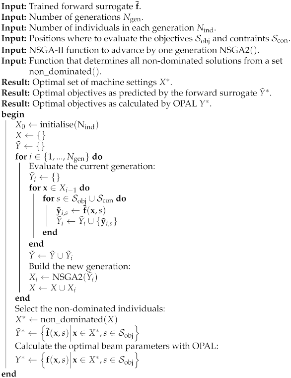
We solve both the AWA and IsoDAR optimisation problems using the NSGA-II algorithm [26] implemented by the Python library pymoo [27], with default parameters. The general algorithm is shown in Algorithm A1. The NSGA 2 ( ) function is given by the quantities of interest for the current generation, calculates the values of the objectives and the constraints and suggests the next generation of machine settings based on the results. When we refer to the optimal solutions of generation g, we refer to the non-dominated feasible solutions that are found in the generations up to and including generation g. Notice that only the forward surrogate model is used to evaluate the objectives and constraints; OPAL is used exclusively to train the models and to validate the final optimal configurations.
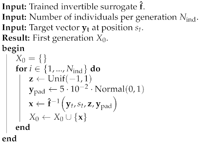
We solved both optimisation problems in two ways: First, we initialised the first generation randomly by uniformly sampling machine settings from their ranges (see Table A3 and Table A4). Second, the invertible model is used to bias the initialisation towards the optimal region. To achieve this, we provided a target vector of beam properties y t at position s t and asked the invertible model to sample the individuals in order to achieve this beam, see Algorithm A2. In other words, we guessed what a good beam would look like at one position, and let the network calculate the corresponding machine settings. This is what allows operators and experimenters to incorporate their experience and intuition into the optimisation.

Appendix D.3. Speedup Calculation

Let t o be the time needed for a single OPAL simulation, running on r o cores. Let t t be the time to train a surrogate model on r t CPU cores, and t p the time needed to evaluate one individual of the optimisation (the p stands for prediction). Assume that the prediction takes place on the same number of cores as the training. Let n be the number of unique machine configurations in the datasets. Since the development of a surrogate model involves a training, validation and test set, all of them are included in this number. Let n h be the number of hyperparameter configurations to be tried for the model. A single optimisation requires running n g generations, each consisting of n i individuals. A summary of the parameters along with their values for both models is depicted in Table A8. The runtime of OPAL depends on the machine settings. The quantity is obtained by measuring the runtime for generating the training/validation set and then dividing by the number of unique machine settings in this set.
Algorithm A1: Optimisation using surrogate models.
Information 12 00351 i001
Algorithm A2: Biased initialisation using the invertible surrogate model.
Information 12 00351 i002
For all calculations, assume that we have infinite computational resources at our disposal. This means that all calculations can always exhaust the entire theoretically available parallelism. In practice, run times are usually higher than the ones calculated using this assumption. The only step where the surrogate model is limited by computational resources is the generation of the dataset. This step is embarrassingly parallel, so the surrogate model can adapt perfectly to limited computational resources. If only OPAL is used, however, the optimisation is also affected by limited resources. In the case where only one individual of a generation cannot be evaluated in parallel to the others, the time needed for the optimisation already doubles. This is because the next generation of the optimisation algorithm cannot start before the parent generation is fully evaluated (assuming that the optimisation algorithm features no parallelism across generations, which is the case for the pymoo implementation). Therefore, our assumption of infinite parallelism favours the OPAL-only approach. For this reason, our calculations result in a lower bound for the speedup.
Table A8. Parameters related to the speedup calculation. For the AWA, the prediction time refers to predicting the beam properties with a spacing of 5 cm, i.e., at 520 positions. For the IsoDAR accelerator, we modelled only 1 position. The times are measured by measuring the prediction time for predicting N m machines and then dividing by N m . For the AWA case, N m = 64 ; for IsoDAR N m = 2 20 .
QuantitySymbolAWAIsoDAR
Time for one OPAL evaluation t o 10 min1.8 h
Time to train one forward model t t 49 h1 h
Time to predict one machine with the surrogate t p 21 ms26 μs
Number of unique machine settings in the datasetn21.0005.000
Number of hyperparameters to try n h 100120
Number of CPU cores per OPAL evaluation r o 41
Number of CPU cores to train and evaluate the surrogate r t 121
Number of generations n g 1.0001.000
Number of individuals per generation n i 200300
Now we can calculate the time-to-solution for an optimisation using the surrogate model. This task involves the creation of the dataset and the model training (including a hyperparameter scan). The former is embarrassingly parallel, and we have unlimited computational resources; thus, all design variable configurations are evaluated at once. The same argument applies for the hyperparameter scan. The time-to-solution for an optimisation with the surrogate model is given by
t surr = t o + t t + n g · t p .
The associated computational cost is calculated as follows
c surr = n · t o · r o + n h · t t · r t + n g · n i · t p · r t .
The time-to-solution for an OPAL optimisation is calculated as
t OPAL = n g · t o .
The corresponding computation cost is calculated by the following
c OPAL = n g · n i · t o · r o .
Now, we can determine the speedup in terms of execution time:
t OPAL t surr = n g · t o t o + t t + n g · t p = n g 1 + t t t o + n g · t p t o n g 1 + t t t o ,
where we have used n g · t p t o 1 for the approximation. This formula can be interpreted as follows: the greater the runtime of OPAL compared to the training time and the more generations we want to calculate for the optimisation, the higher the speedup will be.
The improvement in computational cost can be calculated by
C = c OPAL c surr = n g · n i · t o · r o n · t o · r o + n h · t t · r t + n g · n i · t p · r t .
The relative reduction in computational resources can then be calculated by
c surr c OPAL c OPAL = c surr c OPAL 1 = 1 C 1 .
Solving n optimisation problems is equivalent to solving one problem using n times the number of generations. This means that solving more optimisation problems is equivalent to using more generations. Asymptotically, the improvement in terms of computational cost scales like
C n g t o t p · r o r t .
The relationship of the relative improvement and the number of optimisations can be observed in Figure A3.
Figure A3. Relative improvement in terms of time-to-solution and computational cost for the AWA (a) and the IsoDAR (b) optimisations. The curves are calculated analytically based on measurements of the prediction time for the surrogate model and OPAL.
Information 12 00351 g0a3

References

  1. Shiltsev, V. Particle beams behind physics discoveries. Phys. Today 2020, 73, 32. [Google Scholar] [CrossRef] [Green Version]
  2. No final frontier. Nat. Rev. Phys. 2019, 1, 231. [CrossRef] [Green Version]
  3. Adelmann, A.; Calvo, P.; Frey, M.; Gsell, A.; Locans, U.; Metzger-Kraus, C.; Neveu, N.; Rogers, C.; Russell, S.; Sheehy, S.; et al. OPAL a Versatile Tool for Charged Particle Accelerator Simulations. arXiv 2019, arXiv:1905.06654. [Google Scholar]
  4. Emery, L. Global Optimization of Damping Ring Designs using a Multi-objective Evolutionary Algorithm. In Proceedings of the Particle Accelerator Conference, Knoxville, TN, USA, 16–20 May 2005; p. 2962. [Google Scholar]
  5. Gulliford, C.; Bartnik, A.; Bazarov, I.; Maxson, J. Multiobjective optimization design of an rf gun based electron diffraction beam line. Phys. Rev. Accel. Beams 2017, 20, 033401. [Google Scholar] [CrossRef] [Green Version]
  6. Neveu, N.; Spentzouris, L.; Adelmann, A.; Ineichen, Y.; Kolano, A.; Metzger-Kraus, C.; Bekas, C.; Curioni, A.; Arbenz, P. Parallel general purpose multiobjective optimization framework with application to electron beam dynamics. Phys. Rev. Accel. Beams 2019, 22, 054602. [Google Scholar] [CrossRef] [Green Version]
  7. Frey, M.; Snuverink, J.; Baumgarten, C.; Adelmann, A. Matching of turn pattern measurements for cyclotrons using multiobjective optimization. Phys. Rev. Accel. Beams 2019, 22, 064602. [Google Scholar] [CrossRef] [Green Version]
  8. Kranjčević, M.; Gorgi Zadeh, S.; Adelmann, A.; Arbenz, P.; van Rienen, U. Constrained multiobjective shape optimization of superconducting rf cavities considering robustness against geometric perturbations. Phys. Rev. Accel. Beams 2019, 22, 122001. [Google Scholar] [CrossRef] [Green Version]
  9. Edelen, A.; Neveu, N.; Frey, M.; Huber, Y.; Mayes, C.; Adelmann, A. Machine learning for orders of magnitude speedup in multiobjective optimization of particle accelerator systems. Phys. Rev. Accel. Beams 2020, 23, 044601. [Google Scholar] [CrossRef] [Green Version]
  10. Scheinker, A.; Hirlaender, S.; Velotti, F.M.; Gessner, S.; Della Porta, G.Z.; Kain, V.; Goddard, B.; Ramjiawan, R. Online multi-objective particle accelerator optimization of the AWAKE electron beam line for simultaneous emittance and orbit control. AIP Adv. 2020, 10, 055320. [Google Scholar] [CrossRef]
  11. Jalas, S.; Kirchen, M.; Messner, P.; Winkler, P.; Hübner, L.; Dirkwinkel, J.; Schnepp, M.; Lehe, R.; Maier, A.R. Bayesian Optimization of a Laser-Plasma Accelerator. Phys. Rev. Lett. 2021, 126, 104801. [Google Scholar] [CrossRef]
  12. Power, J. Advanced Acceleration Concepts at the Argonne Wakefield Accelerator Facility. APS Division of Physics of Beams Annual Newsletter. 2018; p. 21. Available online: https://www.anl.gov/awa (accessed on 2 July 2021).
  13. McKay, M.D.; Beckman, R.J.; Conover, W.J. A Comparison of Three Methods for Selecting Values of Input Variables in the Analysis of Output from a Computer Code. Technometrics 1979, 21, 239. [Google Scholar] [CrossRef]
  14. Bungau, A.; Adelmann, A.; Alonso, J.R.; Barletta, W.; Barlow, R.; Bartoszek, L.; Calabretta, L.; Calanna, A.; Campo, D.; Conrad, J.M.; et al. Proposal for an Electron Antineutrino Disappearance Search Using High-Rate 8Li Production and Decay. Phys. Rev. Lett. 2012, 109, 141802. [Google Scholar] [CrossRef] [PubMed]
  15. Waites, L.H.; Alonso, J.R.; Conrad, J. IsoDAR: A cyclotron-based neutrino source with applications to medical isotope production. AIP Conf. Proc. 2019, 2160, 040001. [Google Scholar] [CrossRef]
  16. Alonso, J.R.; Barlow, R.; Conrad, J.M.; Waites, L.H. Medical isotope production with the IsoDAR cyclotron. Nat. Rev. Phys. 2019, 1, 533–535. [Google Scholar] [CrossRef] [Green Version]
  17. Bazarov, I.V.; Sinclair, C.K. Multivariate optimization of a high brightness dc gun photoinjector. Phys. Rev. ST Accel. Beams 2005, 8, 034202. [Google Scholar] [CrossRef] [Green Version]
  18. Veldhuizen, V.; Allen, D. Multiobjective Evolutionary Algorithms: Classifications, Analyses, and New Innovations; Technical Report, Evolutionary Computation; Air Force Institute of Technology: Dayton, OH, USA, 1999. [Google Scholar]
  19. Fonseca, C.M.; Paquete, L.; Lopez-Ibanez, M. An Improved Dimension-Sweep Algorithm for the Hypervolume Indicator. In Proceedings of the 2006 IEEE International Conference on Evolutionary Computation, Vancouver, BC, Canada, 16–21 July 2006; pp. 1157–1163. [Google Scholar] [CrossRef] [Green Version]
  20. Goodfellow, I.; Bengio, Y.; Courville, A. Deep Learning; MIT Press: Cambridge, MA, USA, 2016; Available online: http://www.deeplearningbook.org (accessed on 16 June 2021).
  21. Abadi, M.; Agarwal, A.; Barham, P.; Brevdo, E.; Chen, Z.; Citro, C.; Corrado, G.S.; Davis, A.; Dean, J.; Devin, M.; et al. TensorFlow: Large-Scale Machine Learning on Heterogeneous Systems. 2015. Available online: tensorflow.org (accessed on 3 August 2021).
  22. Liaw, R.; Liang, E.; Nishihara, R.; Moritz, P.; Gonzalez, J.E.; Stoica, I. Tune: A Research Platform for Distributed Model Selection and Training. arXiv 2018, arXiv:1807.05118. [Google Scholar]
  23. Ardizzone, L.; Kruse, J.; Wirkert, S.; Rahner, D.; Pellegrini, E.W.; Klessen, R.S.; Maier-Hein, L.; Rother, C.; Köthe, U. Analyzing Inverse Problems with Invertible Neural Networks. arXiv 2018, arXiv:1808.04730v3. [Google Scholar]
  24. Gretton, A.; Borgwardt, K.M.; Rasch, M.J.; Schölkopf, B.; Smola, A. A kernel two-sample test. J. Mach. Learn. Res. 2012, 13, 723–773. [Google Scholar]
  25. Abs, M.; Adelmann, A.; Alonso, J.R.; Axani, S.; Barletta, W.A.; Barlow, R.; Bartoszek, L.; Bungau, A.; Calabretta, L.; Calanna, A.; et al. IsoDAR@ KamLAND: A Conceptual Design Report for the Technical Facility. arXiv 2015, arXiv:1511.05130. [Google Scholar]
  26. Deb, K.; Pratap, A.; Agarwal, S.; Meyarivan, T. A fast and elitist multiobjective genetic algorithm: NSGA-II. IEEE Trans. Evol. Comput. 2002, 6, 182–197. [Google Scholar] [CrossRef] [Green Version]
  27. Blank, J.; Deb, K. Pymoo: Multi-Objective Optimization in Python. IEEE Access 2020, 8, 89497–89509. [Google Scholar] [CrossRef]
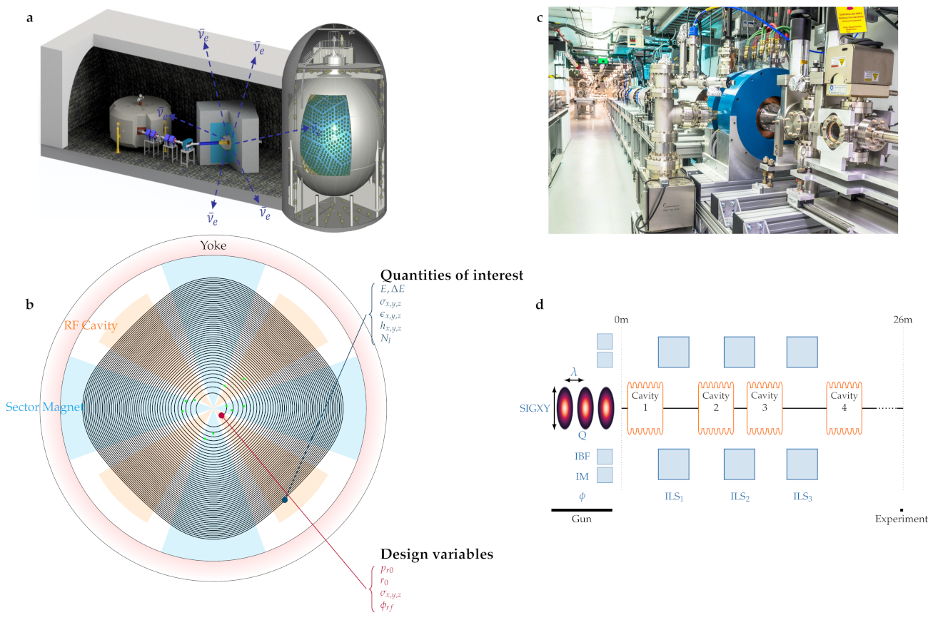
Figure 1. Overview of the use cases. (a) Artistic representation of the IsoDAR experiment at KamLAND (Kamioka Observatory, Japan), from left to right the cyclotron, target and detector are depicted. (b) A schematic of the IsoDAR cyclotron with the relevant parameters. (c) The AWA facility at Argonne National Laboratory (US), pictured from the gun downstream (courtesy of J. Power). (d) Schematic of the relevant parts of the AWA machine.
Information 12 00351 g001
Figure 2. Prediction metrics for the AWA forward surrogate model. The plots show the adjusted coefficient of determination (a) and the relative prediction error (bd) as functions of the longitudinal position. All values are calculated on the test set, i.e., on samples that have not been considered when choosing the parameters. We omit the curves for the QOIs in the y direction for the sake of readability because they are close to the ones in x direction.
Information 12 00351 g002
Figure 3. Optimisations with OPAL (a) and the forward model (b). The gray parts correspond to current practice, the blue parts belong to the genetic algorithm (GA) NSGA-II and the orange parts are our novel contributions. The GA generates n g generations. Schematics of the forward model (c) and invertible model (d) architectures. The grey arrows denote the prediction directions.
Information 12 00351 g003
Figure 4. Convergence of the AWA optimisation. The figures show two-dimensional projections of the objective space (a), i.e., the quantities of interest at 26 m. The shaded area denotes the prediction uncertainty at 90% confidence, and the dots are the predictions themselves. Panels (bd) depict the ranges of objective values among the non-dominated feasible solutions, the volume of the convex hull around the non-dominated solutions plus/minus Monte Carlo uncertainty (e) and the number of non-dominated solutions (f). The colour blue indicates that the optimiser is initialised randomly, and orange indicates that the invertible model is used for the initialisation. All quantities of interest are calculated using the forward surrogate model.
Information 12 00351 g004
Figure 5. OPAL validation of the non-dominated feasible machine settings among all 1000 generations (dots) as calculated using the forward surrogate model. The colour blue marks optimisation with random initialisation, whereas orange indicates that the invertible model provided the initialisation. The dots are the results of an OPAL run, and the shaded areas mark values predicted by the forward model plus/minus uncertainty at 90% confidence.
Information 12 00351 g005
Figure 6. Convergence of the IsoDAR optimisation. The items coloured blue belong to the random initialisation, and the orange ones indicate the usage of the invertible model for initialisation. (a) Two-dimensional projection of the objective space for different generations. The dots are the predictions, and the shaded areas depict the prediction uncertainty at 90% confidence as estimated on the test set. The black circles show the initial values for the biased optimisation. (b) Number of non-dominated solutions. (c) Convergence metrics: Generational Distance (GD) (dots) and Hypervolume Difference (HV diff) (stars) to compare the two optimisation approaches. (d) Range (minimum/maximum) of the non-dominated set in objective space. (e,f) Validation with OPAL. Both figures show the objective space with OPAL validated points in black (triangles), the original OPAL data points in grey (triangles), the 90 percentile (shaded area) of the optimal Pareto front (blue and orange dots) and 100 randomly chosen points of the optimal Pareto front for validation (black dots). (g) Estimated volume of the convex hull of the non-dominated set configurations in objective space using the Monte Carlo uncertainty. The solid lines describe the mean values, and the shaded areas mark the mean plus/minus one standard deviation.
Information 12 00351 g006
Publisher’s Note: MDPI stays neutral with regard to jurisdictional claims in published maps and institutional affiliations.