Article

Improving Imbalanced Land Cover Classification with K-Means SMOTE: Detecting and Oversampling Distinctive Minority Spectral Signatures

NOVA Information Management School (NOVA IMS), Campus de Campolide, Universidade Nova de Lisboa, 1070-312 Lisboa, Portugal
*
Author to whom correspondence should be addressed.
Information 2021, 12(7), 266; https://doi.org/10.3390/info12070266
Submission received: 7 May 2021 / Revised: 22 June 2021 / Accepted: 25 June 2021 / Published: 29 June 2021
(This article belongs to the Special Issue Remote Sensing and Spatial Data Science)

Abstract

:
Land cover maps are a critical tool to support informed policy development, planning, and resource management decisions. With significant upsides, the automatic production of Land Use/Land Cover maps has been a topic of interest for the remote sensing community for several years, but it is still fraught with technical challenges. One such challenge is the imbalanced nature of most remotely sensed data. The asymmetric class distribution impacts negatively the performance of classifiers and adds a new source of error to the production of these maps. In this paper, we address the imbalanced learning problem, by using K-means and the Synthetic Minority Oversampling Technique (SMOTE) as an improved oversampling algorithm. K-means SMOTE improves the quality of newly created artificial data by addressing both the between-class imbalance, as traditional oversamplers do, but also the within-class imbalance, avoiding the generation of noisy data while effectively overcoming data imbalance. The performance of K-means SMOTE is compared to three popular oversampling methods (Random Oversampling, SMOTE and Borderline-SMOTE) using seven remote sensing benchmark datasets, three classifiers (Logistic Regression, K-Nearest Neighbors and Random Forest Classifier) and three evaluation metrics using a five-fold cross-validation approach with three different initialization seeds. The statistical analysis of the results show that the proposed method consistently outperforms the remaining oversamplers producing higher quality land cover classifications. These results suggest that LULC data can benefit significantly from the use of more sophisticated oversamplers as spectral signatures for the same class can vary according to geographical distribution.

1. Introduction

The increasing amount of remote sensing missions granted the access to dense time series (TS) data at a global level and provides up-to-date, accurate land cover information [1]. This information is often materialized through Land Use and Land Cover (LULC) maps. While Land Cover maps define the biophysical cover found on the surface of the earth, Land Use maps define how it is used by humans [2]. Both Land Use and Land Cover maps constitute an essential asset for various purposes, such as land cover change detection, urban planning, environmental monitoring and natural hazard assessment [3]. However, the timely production of accurate and updated LULC maps is still a challenge within the remote sensing community [4]. LULC maps are produced based on two main approaches: photo-interpreted by the human eye, or automatic mapping using remotely sensed data and classification algorithms.
While photo-interpreted LULC maps rely on human operators and can be more reliable, they also present some significant disadvantages. The most important disadvantage is the cost of production, in fact photo-interpretation consumes significant resources, both in terms of money and time. Because of that, they are not frequently updated and not suitable for operational mapping over large areas. Finally, there is also the issue of overlooking rare or small-area classes, due to factors such as the minimum mapping unit being used.
Automatic mapping with classification algorithms based on machine-learning (ML) has been extensively researched and used to speed up and reduce the costs of the production process [3,5,6]. Improvements in classification algorithms are sure to have a significant impact on the efficiency with which remote sensing imagery is used. Several challenges have been identified in order to improve automatic classification:
  • Improve the ability to handle high-dimensional datasets, in cases such as Multi-spectral TS composites high-dimensionality increases the complexity of the problem and creates a strain on computational power [7].
  • Improve class separability, as the production of an accurate LULC map can be hindered by the existence of classes with similar spectral signatures, making these classes difficult to distinguish [8].
  • Resilience to mislabelled LULC patches, as the use of photo-interpreted training data poses a threat to the quality of any LULC map produced with this strategy, since factors such as the minimum mapping unit tend to cause the overlooking of small-area LULC patches and generates noisy training data that may reduce the prediction accuracy of a classifier [9].
  • Dealing with rare land cover classes, due to the varying levels of area coverage for each class. In this case using a purely random sampling strategy will amount to a dataset with a roughly proportional class distribution as the one on the multi/hyperspectral image. On the other hand, the acquisition of training datasets containing balanced class frequencies is often unfeasible. This causes an asymmetry in class distribution, where some classes are frequent in the training dataset, while others have little expression [10,11].
The latter challenge is known, in machine learning, as the imbalanced learning problem [12]. It is defined as a skewed distribution of instances found in a dataset among classes in both binary and multi-class problems [13]. This asymmetry in class distribution negatively impacts the performance of classifiers, especially in multi-class problems. The problem comes from the fact that during the learning phase, classifiers are optimized to maximize an objective function, with overall accuracy being the most common one [14]. This means that instances belonging to minority classes contribute less to the optimization process, translating into a bias towards majority classes. As an example, a trivial classifier can achieve 99% overall accuracy on a binary dataset where 1% of the instances belong to the minority class if it classifies all instances as belonging to the majority class. This is an especially significant issue in the automatic classification of LULC maps, as the distribution of the different land-use classes tends to be highly imbalanced. Therefore, improvements in the ability to deal with imbalanced datasets will translate into important progress in the automatic classification of LULC maps.
There are three different types of approaches to deal with the class imbalance problem [6,15]:
  • Cost-sensitive solutions. Introduces a cost matrix to the learning phase with misclassification costs attributed to each class. Minority classes will have a higher cost than majority classes, forcing the algorithm to be more flexible and adapt better to predict minority classes.
  • Algorithmic level solutions. Specific classifiers are modified to reinforce the learning on minority classes. Consists on the creation or adaptation of classifiers.
  • Resampling solutions. Rebalances the dataset’s class distribution by removing majority class instances and/or generating artificial minority instances. This can be seen as an external approach, where the intervention occurs before the learning phase, benefitting from versatility and independency from the classifier used.
Since resampling strategies represent a set of methods that are detached from classifiers by operating at the data level, they allow the use of any off the shelf algorithm, without the need for any type of changes or adaptions to the algorithm. Specifically, in the case of oversampling (defined below), the user is able to balance the dataset’s class distribution by without the loss of information, which is not the case with undersampling techniques. This is a significant advantage especially considering that most users in remote sensing are not expert machine learning engineers.
Within resampling approaches there are three subgroups of approaches [6,15,16]:
  • Undersampling methods, which rebalance class distribution by removing instances from the majority classes.
  • Oversampling methods, which rebalance datasets by generating new artificial instances belonging to the minority classes.
  • Hybrid methods, which are a combination of both oversampling and undersampling, resulting in the removal of instances in the majority classes and the generation of artificial instances in the minority classes.
Resampling methods can be further distinguished between non-informed and heuristic (i.e., informed) resampling techniques [15,16,17]. The former consist of methods that duplicate/remove a random selection of data points to set class distributions to user-specified levels, and are therefore a simpler approach to the problem. The latter consists of more sophisticated approaches that aim to perform over/undersampling based on the points’ contextual information within their data space.
The imbalanced learning problem is not new in machine learning but its relevancy has been growing, as attested by [18]. The problem has also been addressed in the context of remote sensing [19]. In this paper, we propose the application of a recent oversampler based on SMOTE [20], the K-means SMOTE [21] oversampler, to address the imbalanced learning problem in a multiclass context for LULC classification using various remote sensing datasets. Specifically, we use seven land use datasets commonly used in research literature, that vary among agricultural and urban land use. The K-means SMOTE algorithm couples two different procedures in the generation of artificial data. The algorithm starts by grouping the instances into clusters by using the K-means algorithm; next, the generation of the artificial data is done using the smote algorithm, taking into consideration the distribution of majority/minority cases in each individual cluster. The idea of starting with a clustering procedure before the data generation phase is important in remote sensing because the spectral signature of the different classes can change significantly based on the geographical area in which it is represented. In other words, the spectral signature of a specific class can vary greatly depending on the geography, meaning that often we will be facing within-class imbalance [22].
In fact, we can decompose class imbalance into two different types: between-class imbalance and within-class imbalance [21,23]. While the first refers to the overall asymmetry between majority and minority classes, the second results from the fact that in different areas of the input space there might be different levels of imbalance. Depending on the complexity of the input space, different subclusters of minority and majority instances may be present. In order to achieve a balance between minority and majority instances, these subclusters should be treated separately. Assuming that the role of a classifier is to create rules in such a way that it is able to isolate the different relevant sub-concepts that represent both the majority and minority classes, the classifier will create multiple disjunct rules that describe these concepts. If the input space is simple and the classes’ instances are grouped together in a unique cluster, the classifier will only need to create (general) rules that comprise large portions of instances belonging to the same class. To the contrary, if the input space is complex and scatters through multiple small clusters, the classifier will need to learn a more complex set of (specific) rules, which can be seen in Figure 1. It is important to note that small clusters can happen both in the minority and majority class, although they will tend to be more frequent in the minority class due to its underrepresentation.
The efficacy of K-means SMOTE is tested using different types of classifiers. To do so, we employ both commonly used and/or state-of-the-art oversamplers as benchmarking methods: random oversampling (ROS), SMOTE and Borderline-SMOTE (B-SMOTE) [24]. Additionally, as a baseline score we include classification results without the use of any resampling method.
This paper is organized in 5 sections: Section 2 provides an overview of the state-of-art, Section 3 describes the proposed methodology, Section 4 covers the results and discussion and Section 5 presents the conclusions taken from this study.
This paper’s main contributions are:
  • Propose a cluster-based multiclass oversampling method appropriate for LULC classification and compare its performance with the remaining oversamplers in a multiclass context with seven benchmark LULC classification datasets. Allows us to check the oversamplers’ performance across benchmark LULC datasets.
  • Introducing a cluster-based oversampling algorithm within the remote sensing domain, as well as comparing its performance with the remaining oversamplers in a multiclass context.
  • Make available to the remote sensing community the implementation of the algorithm in a Python library and the experiment’s source code.

2. Imbalanced Learning Approaches

Imbalanced learning has been addressed in three different ways: over/undersampling, cost-sensitive training and changes/adaptations in the learning algorithms [6]. These approaches impact different phases of the learning process, while over/undersampling can be seen as a pre-processing step, cost-sensitive and changes in the algorithm imply a more customized and complex intervention in the algorithms. In this section, we focus on previous work related with resampling methods, while providing a brief explanation of cost-sensitive and algorithmic level solutions.
All of the most common classifiers used for LULC classification tasks [3,5] are sensitive to class imbalance [25]. Algorithm-based approaches typically focus on adaptations based on ensemble classification methods [26] or common non-ensemble based classifiers such as Support Vector Machines [27]. In [28], the reported results show that algorithm-based methods have comparable performance to resampling methods.
Cost-sensitive solutions refer to changes in the importance attributed to each instance through a cost matrix [29,30,31]. A relevant cost sensitive solution [29] uses the inverse class frequency (i.e., 1 / | C i | , where C i refers to the frequency of class i) to give higher weight to minority classes. Cui et al. [30] extended this method by adding a hyperparameter β to class weights as ( 1 β ) / ( 1 β | C i | ) . When β = 0 , no re-weighting is done. When β 1 , weights are the inverse of the frequency class matrix. Another method [31] explores adaptations of cross-entropy classification loss by adding different formulations of class rectification loss.
Resampling (over/undersampling) is the most common approach to imbalanced learning in machine learning in general and remote sensing in particular [11]. The generation of artificial instances (i.e., augmenting the dataset), based on rare instances, is done independently of any other step in the learning process. Once the procedure is applied, any standard machine learning algorithm can be used. Its simplicity makes resampling strategies particularly appealing for any user (especially the non-sophisticated user) interested in applying several classifiers, while maintaining a simple approach. It is also important to notice that over/undersampling methods can also be easily applied to multiclass problems, common in LULC classification tasks.

2.1. Non-Informed Resampling Methods

There are two main non-informed resampling methods. Random Oversampling (ROS) generates artificial instances through random duplication of minority class instances. This method is used in remote sensing for its simplicity [32,33], even though its mechanism makes the classifier prone to overfitting [34]. Ref. [33] found that using ROS returned worse results than keeping the original imbalance in their dataset.
A few of the recent remote sensing studies employed Random Undersampling (RUS) [35], which randomly removes instances belonging to majority classes. Although it’s not as prone to overfitting as ROS, it incurs into information loss by eliminating instances from the majority class [11], which can be detrimental to the quality of the results.
Another disadvantage of non-informed resampling methods is their performance-wise inconsistency across classifiers. ROS’ impact on the Indian Pines dataset was found inconsistent between Random Forest Classifiers (RFC) and Support Vector Machines (SVM) and lowered the predictive power of an artificial neural network (ANN) [14]. Similarly, RUS is found to generally lead to a lower overall accuracy due to the associated information loss [14].

2.2. Heuristic Methods

The methods presented in this section appear as a means to overcome the insufficiencies found in non-informed resampling. They use either local or global information to generate new, relevant, non-duplicated instances to populate the minority classes and/or remove irrelevant instances from majority classes. In a comparative analysis between over- and undersamplers’ performance for LULC classification [36] using the rotation forest ensemble classifier, authors found that oversampling methods consistently outperformed undersampling methods. This result led us to exclude undersampling from our study.
SMOTE [20] was the first heuristic oversampling algorithm to be proposed and has been the most popular one since then, likely due to its fair degree of simplicity and quality of generated data. It takes a random minority class sample and introduces synthetic instances along the line segment that join a random k minority class nearest neighbor to the selected sample. Specifically, a single synthetic sample z is generated within the line segment of a randomly selected minority class instance x and one of its k nearest neighbors y such that z = α x + ( 1 α ) y , where α is a random real number between 0 and 1, as shown in Figure 2.
A number of studies implement SMOTE within the LULC classification context and reported improvements on the quality of the trained predictors [37,38]. Another study proposes an adaptation of SMOTE on an algorithmic level for deep learning applications [39]. This method combines both typical computer vision data augmentation techniques, such as image rotation, scaling and flipping on the generated instances to populate minority classes. Another algorithmic implementation is the variational semi-supervised learning model [40]. It consists of a generative model that allows learning from both labeled and unlabeled instances while using SMOTE to balance the data.
Despite SMOTE’s popularity, its limitations have motivated the development of more sophisticated oversampling algorithms [21,24,41,42,43,44]. Ref. [41] identify four major weaknesses of the SMOTE algorithm, which can be summarized as:
  • Generation of noisy instances due to random selection of a minority instance to oversample. The random selection of a minority instance makes SMOTE oversampling prone to the amplification of existing noisy data. This has been addressed by variants such as B-SMOTE [24] and ADASYN [44].
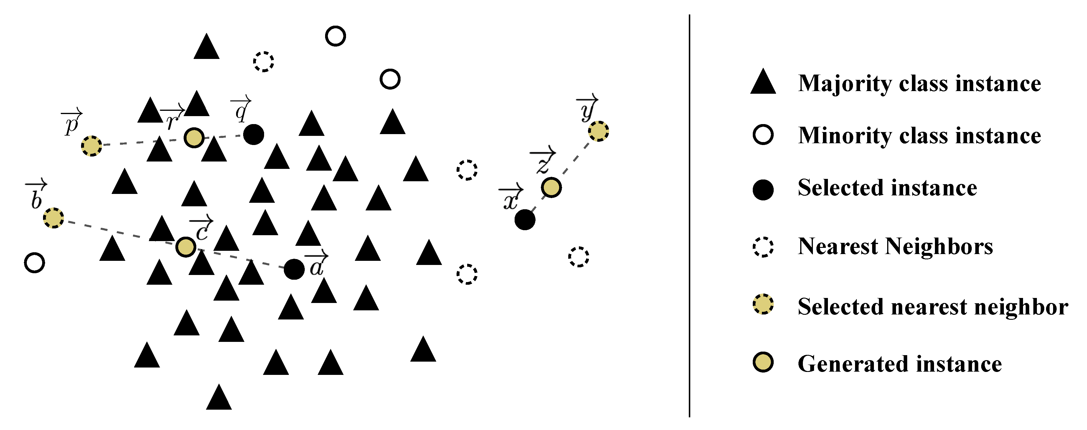
  • Generation of noisy instances due to the selection of the k nearest neighbors. In the event an instance (or a small number thereof) is not noisy but is isolated from the remaining clusters, known as the “small disjuncts problem” [45], much like sample b from Figure 2, the selection of any nearest neighbor of the same class will have a high likelihood of producing a noisy sample.
  • Generation of nearly duplicated instances. Whenever the linear interpolation is done between two instances that are close to each other, the generated instance becomes very similar to its parents and increases the risk of overfitting. G-SMOTE [41] attempts to address both the k nearest neighbor selection mechanism problem as well as the generation of nearly duplicated instances problem.
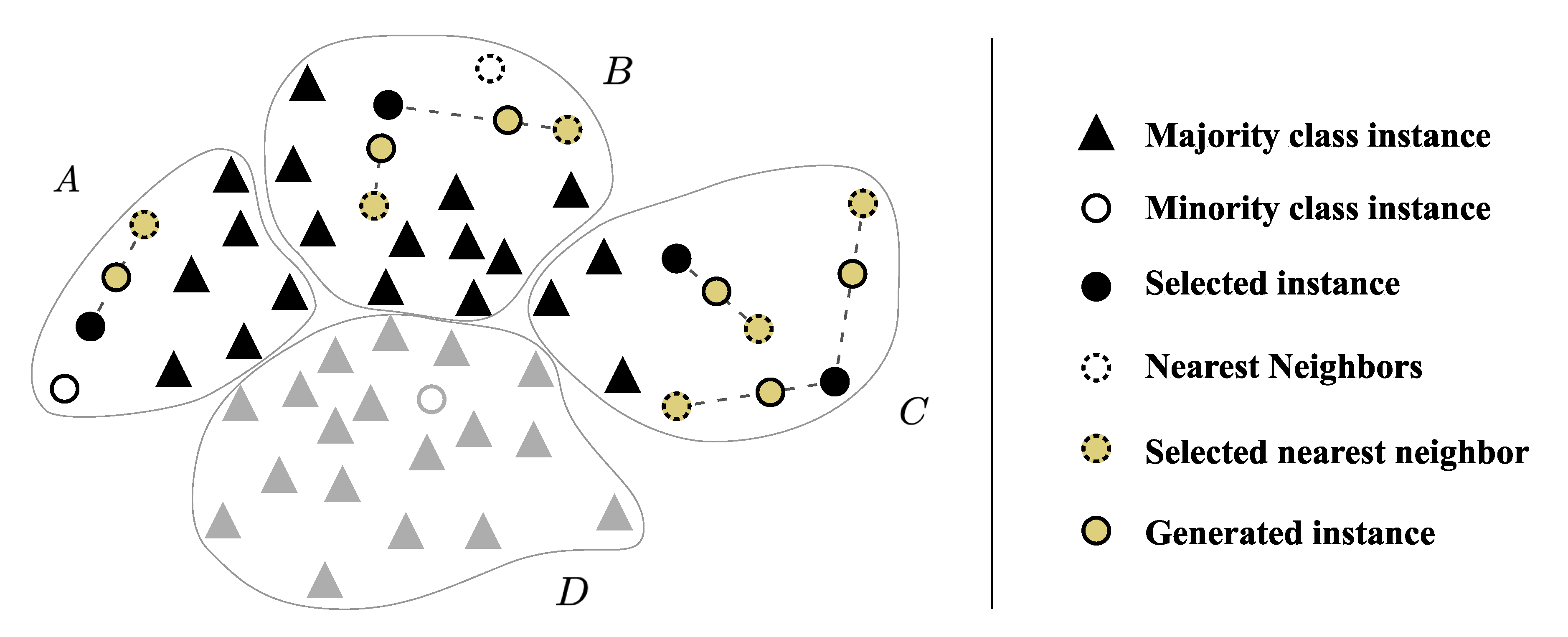
  • Generation of noisy instances due to the use of instances from two different minority class clusters. Although an increased k could potentially avoid the previous problem, it can also lead to the generation of artificial data between different minority clusters, as depicted Figure 2 with the generation of point r using minority class instances p and q . Cluster-based oversampling methods attempt to address this problem.
This last issue, the generation of noisy instances due to the existence of several minority class clusters, is particularly relevant in remote sensing. It is frequent that instances belonging to the same minority class can have different spectral signatures, meaning that they will be clustered in different parts of the input space. For example, in the classification of a hyperspectral scene dominated by agricultural activities, patches relating to urban areas may constitute a minority class. These patches frequently refer to different types of land use, such as housing regions, small gardens, asphalt roads, etc., all these containing different spectral signatures. In this context, the use of SMOTE will lead to the generation of noisy instances of the minority class. This problem can be efficiently mitigated through the use of a cluster-based oversampling method. According to our literature review cluster-based oversampling approaches have never been applied in the context of remote sensing. On the other hand, while there are references of the application of cluster-based oversampling in the context of machine learning [21,42,43,46], the multiclass case is rarely addressed, which is a fundamental requirement for the application of oversampling in the context of LULC.
Cluster-based oversampling approaches introduce an additional layer to SMOTE’s selection mechanism, which is done through the inclusion of a clustering process. This ensures that both between-class data balance and within-class balance is preserved. The self-organizing map oversampling (SOMO) [43] algorithm transforms the dataset into a 2-dimensional input, where the areas with the highest density of minority samples are identified. SMOTE is then used to oversample each of the identified areas separately. Clustered Resampling SMOTE (CURE-SMOTE) [42] applies a hierarchical clustering algorithm to discard isolated minority instances before applying SMOTE. Although it avoids noise generation problems, it ignores within-class data distribution. Another method [46] uses K-means to cluster the entire input space and applies SMOTE to clusters with the fewest instances, regardless of their class label. The label of the generated instance is copied from one of its parents. This method cannot ensure a balanced dataset since class imbalance is not specifically addressed, but rather dataset imbalance.
K-means SMOTE [21] avoids noisy data generation by modifying the data selection mechanism. It employs k-means clustering to identify safe areas using cluster-specific Imbalance Ratio (IR, defined by c o u n t ( C m a j o r i t y ) c o u n t ( C m i n o r i t y ) ) and determine the quantity of generated samples per cluster based on a density measure. These samples are finally generated using the SMOTE algorithm. The K-means SMOTE’s data generation process is depicted in Figure 3. Note that the number of samples generated for each cluster varies according to the sparsity of each cluster (the sparser the cluster is, the more samples will be generated) and a cluster is rejected if the cluster’s IR surpasses the threshold. Therefore, this method can be combined with any data generation mechanism, such as G-SMOTE. Additionally, K-means SMOTE includes the SMOTE algorithm as a special case when the number of clusters is set to one. Consequently, K-means SMOTE returns results as good as or better than SMOTE.
Although no other study was found to implement cluster-based oversampling, another study [19] compared the performance of SMOTE, ROS, ADASYN, B-SMOTE and G-SMOTE in a highly imbalanced LULC classification dataset. The authors found that G-SMOTE consistently outperformed the remaining oversampling algorithms regardless of the classifier used.

3. Methodology

The purpose of this work is to understand the performance of K-means SMOTE as opposed to other popular and/or state-of-the-art oversamplers for LULC classification. This was done using seven datasets with predominantly land use information, along with three evaluation metrics and three classifiers to evaluate the performance of oversamplers. In this section we describe the datasets, evaluation metrics, oversamplers, classifiers and software used as well as the procedure developed.

3.1. Datasets

The datasets used were extracted from publicly available hyperspectral scenes. Information regarding each of these scenes is provided in this subsection. The data collection and preprocessing pipeline is shown in Figure 4 and is common to all hyperspectral scenes:
  • Data collection of publicly available hyperspectral scenes. The original hyperspectral scenes and ground truth data were collected from a single publicly available data repository available here (http://www.ehu.eus/ccwintco/index.php?title=Hyperspectral_Remote_Sensing_Scenes (accessed on 29 June 2021)).
  • Conversion of each hyperspectral scene to a structured dataset and removal of instances with no associated LULC class. This was done to reshape the dataset from ( h , w , b + g t ) into a conventional dataframe of shape ( h w , b + g t ) , where g t , h, w and b represent the ground truth, height, width and number of bands in the scene, respectively. The pixels without ground truth information were discarded from further analysis.
  • Stratified random sampling to maintain similar class proportions on a sample of 10% of each dataset. This was done by computing the relative class frequencies in the original hyperspectral scene (minus the class representing no ground truth availability) and retrieving a sample that ensured the original relative class frequencies remained unchanged.
  • Removal of instances belonging to a class with frequency lower than 20 or higher than 1000. This was done to maintain the datasets to a practicable size due to computational constraints, while conserving the relative LULC class frequencies and data distribution.
  • Data normalization using the MinMax scaler. This ensured all features (i.e., bands) were in the same scale. In this case, the data were rescaled between 0 and 1.
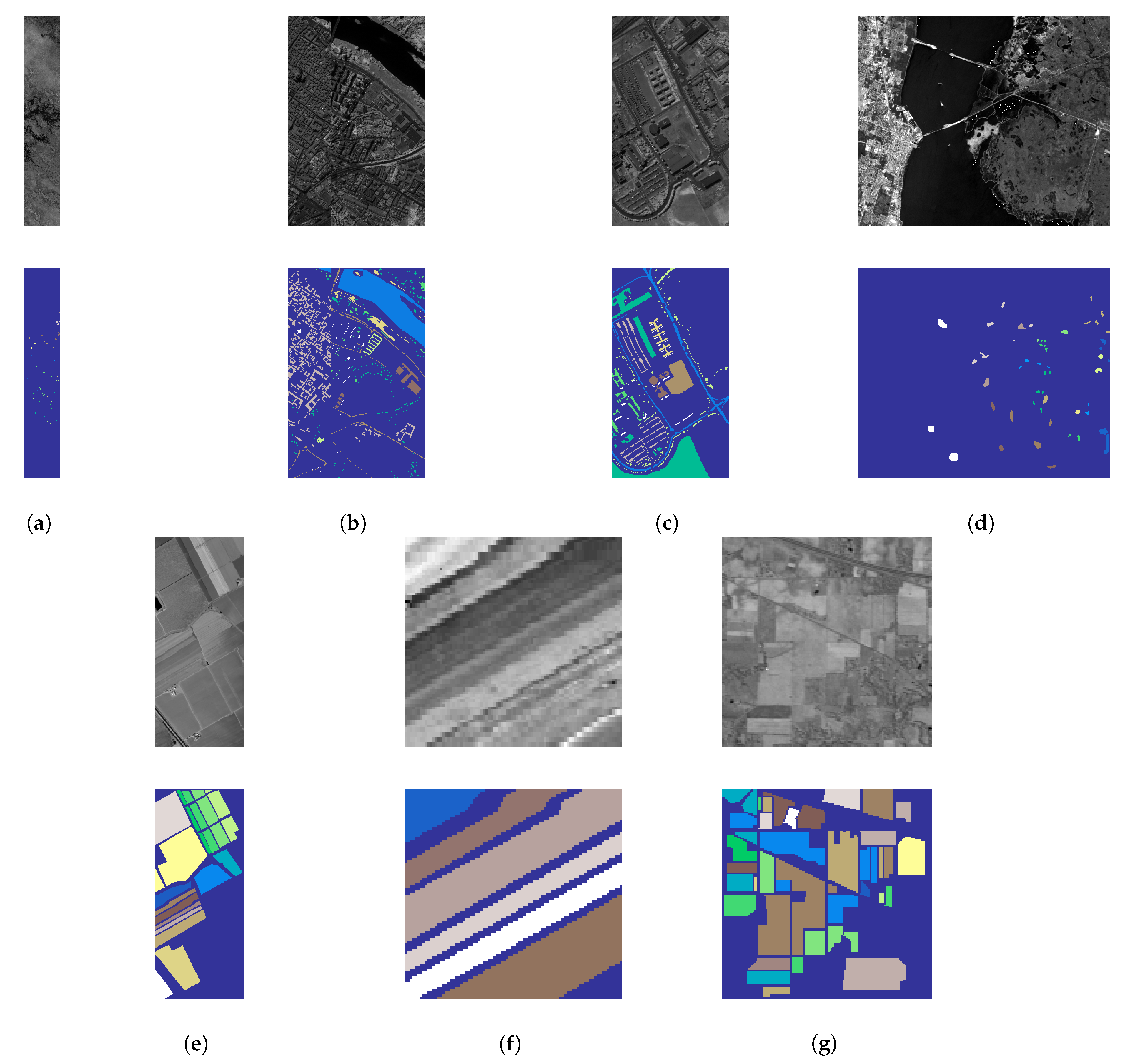
Table 1 provides a description of the final datasets used for this work, sorted according to its IR. Figure 5 shows the original hyperspectral scene out of which the dataset used in this experiment was extracted. In the representation of the ground truth of these scenes, the blue regions in the ground truth of each hyperspectral scene represent unlabeled regions (i.e., no ground truth was available). Particularly, in the Botswana and Kennedy Space Center scenes the truth was photointerpreted in more limited regions of the scene. However, the scenes are still represented as they were in order to maintain a standardized analysis over all datasets extracted for the experiment.

3.1.1. Botswana

The Botswana scene was acquired by the Hyperion sensor on the NASA EO-1 satellite over the Okavango Delta, Botswana in 2001–2004 at a 30 m spatial resolution. Data preprocessing was performed by the UT Center for Space Research. The scene comprised a 1476 × 256 pixels with 145 bands and 14 classes regarding land cover types in seasonal and occasional swamps, as well as drier woodlands (see Figure 5a). The classes with rare instances were Short mopane and Hippo grass.

3.1.2. Pavia Center and University

Both Pavia Center and University scenes were acquired by the ROSIS sensor. These scenes were located in Pavia, northern Italy. Pavia Center is a 1096 × 1096 pixels image with 102 spectral bands, whereas Pavia University is a 610 × 610 pixels image with 103 spectral bands. Both images had a geometrical resolution of 1.3 m and their ground truths were composed of nine classes each (see Figure 5b,c). After data preprocessing, the classes with rare instances were Asphalt and Bitumen (the class Shadows was removed for being too rare for cross validation after random sampling).

3.1.3. Kennedy Space Center

The Kennedy Space Center scene was acquired by the AVIRIS sensor over the Kennedy Space Center, Florida, on 23 March 1996. Out of the original 224 bands, water absorption and low SNR bands were removed and a total of 176 bands at a spatial resolution of 18 m were used. The scene was a 512 × 614 pixel image and contains a total of 16 classes (see Figure 5d). The classes with rare instances were hardwood swamp, slash pine and willow swamp (both hardwood swamp and slash pine were removed for being too rare for cross validation after random sampling).

3.1.4. Salinas and Salinas-A

These scenes were collected by the AVIRIS sensor over Salinas Valley, California and contain at-sensor radiance data. Salinas was a 512 × 217 pixels image with 224 bands and 16 classes regarding vegetables, bare soil and vineyard fields (see Figure 5e). Salinas-A, a subscene of Salinas, comprised 86 × 83 pixels and contained six classes regarding vegetables (see Figure 5f). These scenes had a geometrical resolution of 3.7 m. Salinas-A’s minority class had the label “Brocoli_green_weeds_1” and Salina’s minority class had the label “Lettuce_romaine_6wk”.

3.1.5. Indian Pines

The Indian Pines scene [47] was collected on 12 June 1992 and consists of AVIRIS hyperspectral image data covering the Indian Pine Test Site 3, located in North-western Indiana, USA. As a subset of a larger scene, it was composed of 145 × 145 pixels (see Figure 5g) and 220 spectral reflectance bands in the wavelength range 400 to 2500 nanometers at a spatial resolution of 20 m. Approximately two thirds of this scene was composed of agriculture and the other third was composed of forest and other natural perennial vegetation. Additionally, the scene also contained low density buildup areas. The classes with rare instances were Alfalfa, Oats, Grass-pasture-mowed, Wheat and Stone-Steel-Towers (which was removed for being too rare for cross validation after random sampling). After data preprocessing, the classes with rare instances were Corn, Buildings-Grass-Trees-Drives and Grass-Pasture.

3.2. Machine Learning Algorithms

To assess the quality of the K-means SMOTE algorithm, three other oversampling algorithms were used for benchmarking. ROS and SMOTE were chosen for their simplicity and popularity. B-SMOTE chosen as a popular variation of the SMOTE algorithm. We also include the classification results of no oversampling (NONE) as a baseline.
To assess the performance of each oversampler, we use the classifiers Logistic Regression (LR) [48], K-Nearest Neighbors (KNN) [49] and Random Forest (RF) [50]. This choice was based on the classifiers’ popularity for LULC classification, learning type and training time [5,14]. Since this is a multinomial classification task, for the LR classification we adopted a one-versus-all approach for each label. The predicted label is assigned according to the class predicted with highest probability.

3.3. Evaluation Metrics

Most of the satellite-based LULC classification studies (nearly 80%) employ Overall Accuracy (OA) and the Kappa Coefficient [5]. Although, some authors argue that both evaluation metrics, even when used simultaneously, are insufficient to fully address the area estimation and uncertainty information needs [51,52]. Other metrics like User’s Accuracy (or Precision) and Producer’s Accuracy (or Recall) are also common metrics to evaluate per-class prediction power. These metrics consist of ratios employing the True and False Positives (TP and FP, number of correctly/incorrectly classified instances of a given class) and True and False Negatives (TNs and FNs, number of correctly/incorrectly classified instances as not belonging to a given class). These metrics are formulated as P r e c i s i o n = T P T P + F P and R e c a l l = T P T P + F N . While metrics like OA and Kappa Coefficient are significantly affected by imbalanced class distributions, F-Score is less sensitive to data imbalance and a more appropriate choice for performance evaluation [53].
The datasets used presented significantly high IRs (see Table 1). Therefore, it was especially important to attribute equal importance to the predictive power of all classes, which did not happen with OA and Kappa Coefficient. In this study, we employed three evaluation metrics: (1) G-mean, since it was not affected by skewed class distributions, (2) F-Score, as it proved to be a more appropriate metric for this problem when compared to other commonly used metrics [53], and (3) Overall Accuracy, for discussion purposes.
  • The G-mean consists of the geometric mean of S p e c i f i c i t y = T N T N + F P and Sensitivity (also known as Recall). For multiclass problems, The G-mean is expressed as:
    G - mean = S e n s i t i v i t y ¯ × S p e c i f i c i t y ¯
  • F-score is the harmonic mean of Precision and Recall. The F-score for the multi-class case can be calculated using their average per class values [54]:
    F - score = 2 P r e c i s i o n ¯ × R e c a l l ¯ P r e c i s i o n ¯ + R e c a l l ¯
  • Overall Accuracy is the number of correctly classified instances divided by the total amount of instances. Having c as the label of the various classes, Accuracy is given by the following formula:
    Accuracy = c TP c c ( TP c + FP c )
In the case of G-mean and F-score, both metrics are computed for each label and their unweighted mean is calculated (i.e., following a “macro” approach). In this study we assume that all labels have an equivalent importance for the classification task.

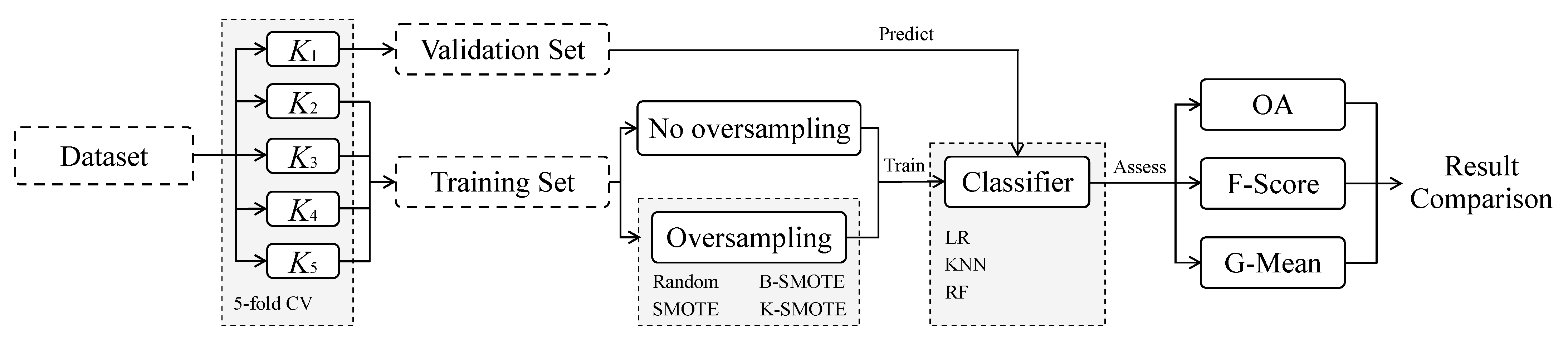
3.4. Experimental Procedure

The procedure for the experiment started with the definition of a hyperparameter search grid, where a list of possible values for each relevant hyperparameter in both classifiers and oversamplers was stored. Based on this search grid, all possible combinations of oversamplers, classifiers and hyperparameters were formed. Finally, for each dataset, hyperparameter combination and initialization we used the evaluation strategy shown in Figure 6: k-fold cross-validation strategy where k = 5 to train each model defined and save the averaged scores of each split.
In the five-fold cross validation strategy, a combination of oversampler, classifier and hyperparameters vector was fit five times per dataset. Before the training phase, the training set (containing 4 5 of the dataset) was oversampled using one of the methods described (except for the baseline method NONE), creating an augmented dataset with the exact same number of instances for each class. The newly formed training dataset was used to train the classifier and the test set ( 1 5 of the dataset) was used to evaluate the performance of the classifier. The evaluation scores were then averaged over the five times the process was repeated. The range of hyperparameters used are shown in Table 2. The definition of hyperparameters for the K-means SMOTE oversampler was defined according to the recommendations discussed in the original K-means SMOTE paper [21].

3.5. Software Implementation

The experiment was implemented using the Python programming language, using the Scikit-Learn (https://scikit-learn.org/stable/ (accessed on 29 June 2021)) [55], Imbalanced-Learn (https://imbalanced-learn.org/stable/ (accessed on 29 June 2021)) [56], Geometric-SMOTE (https://geometric-smote.readthedocs.io/en/latest/?badge=latest (accessed on 29 June 2021)), Cluster-Over-Sampling (https://cluster-over-sampling.readthedocs.io/en/latest/?badge=latest (accessed on 29 June 2021)) and Research-Learn (https://research-learn.readthedocs.io/en/latest/?badge=latest (accessed on 29 June 2021)) libraries. All functions, algorithms, experiments and results are provided at the GitHub repository of the project (https://github.com/AlgoWit/publications (accessed on 29 June 2021)).

4. Results and Discussion

When evaluating the performance of an algorithm across multiple datasets, it is generally recommended to avoid direct score comparisons and use classification rankings instead [57]. This was done by assigning a ranking to oversamplers based on the different combinations of classifier, metric and dataset used. These rankings were also used for the statistical analyses presented in Section 4.2.
The rank values were assigned based on the mean validation scores resulting from the experiment described in Section 3. The averaged ranking results were computed over three different initialization seeds and a five fold cross validation scheme, returning a real number within the interval [ 1 ,   5 ] .
The hyperparameter optimization ensured that both oversamplers and classifiers were well adapted to each of the datasets used in the experiment. Specifically, the optimization of classifiers’ hyperparameters was not particularly relevant since our focus was to study the relative performance scores across oversamplers. This provided insights on the quality of the artificial data generated by each oversampler. The classifiers’ hyperparameter tuning was done to avoid the over/underfitting of classifiers, since they were trained on the same data subsets along with artificial data generated with different methods.

4.1. Results

The mean ranking of oversamplers is presented in Figure 7. This ranking was computed by averaging the ranks of the mean cross-validation scores per dataset, oversampler and classifier. K-means SMOTE achieved the best mean ranking across datasets with low standard deviation.
The mean cross-validation scores are shown in Table 3. As discussed previously in this section, the disparity of performance levels across datasets made the analysis of these scores less informative.
The mean cross-validation scores for each dataset are presented in Table A1 (see Appendix A). This table allows the direct comparison of the performance metrics being analyzed.

4.2. Statistical Analysis

The experiment’s multi-dataset context was used to perform a Friedman test [58]. Table 4 shows the results obtained in the Friedman test performed, where the null hypothesis was rejected in all cases. The rejection of the null hypothesis implies that the differences between the differences among the different oversamplers were not random, in other words, these differences were statistically significant.
A Wilcoxon signed-rank test [59] was also performed to understand whether K-means SMOTE’s superiority was statistically significant across datasets and oversamplers, as suggested in [57]. This method was used as an alternative to the paired Student’s t-test, since the distribution of the differences between the two samples cannot be assumed as normally distributed. The null hypothesis of the test was that K-means SMOTE’s performance was similar to the compared oversampler (i.e., the oversamplers used followed a symmetric distribution around zero).

4.3. Discussion

The mean rankings presented in Figure 7 show that on average, K-means SMOTE produced the best results for every classifier and performance metric used. This is due to the clustering phase and subsequent selection of data to be considered for oversampling. By successfully clustering and selecting the relevant areas in the data space to oversample, the generation of artificial instances is done only in the context of minority regions that represent well their spectral signature.
As previously discussed, the direct comparison of performance metrics averaged over various datasets is not recommended due to the varying levels of performance of classifiers across datasets [57]. Nonetheless, these results are shown in Table 3 to provide a fuller picture of the results obtained in the experiment. We found that on average K-means SMOTE provides increased performance, regardless of the classifier and performance metric used. More importantly, K-means SMOTE guaranteed a more consistent performance across datasets and with less variability, which can be attested in Figure 7 and Table 3 and Table A1.
As discussed in Section 3.3, Evaluation Metrics, our results are consistent with the findings in [51,52]. Particularly, we consider the results obtained in our experiment using Overall Accuracy to be less informative than the results obtained with the remaining performance metrics, since this metric is affected by imbalanced class distributions. The majority class bias in this metric can be observed in our experiment in Figure 7 with the classifiers LR and KNN, where the control method (NONE) is only outperformed by K-means SMOTE. This effect is observed with more detail in Table 3, where the benchmark oversamplers are outperformed by the control method in 16 out of 63 tests (approximately 25%). Out of these, most refer to tests using overall accuracy among the four datasets with highest IR, showing the overall accuracy’s class imbalance bias discussed in [51,52]. The K-means SMOTE oversampler is only outperformed by the control method in 3 of tests (all of them using overall accuracy). This is an improvement over the benchmark oversamplers, showing that generally K-means SMOTE is the best choice even when overall accuracy is used as the main performance metric.
In the majority of the cases, K-means SMOTE was able to generate higher quality data due to the non-random selection of data spaces to oversample. This can be seen in the performance of the classifiers trained on top of this data generation step, making it a more informed data generation method in the context of LULC.
The performance of both oversamplers and classifiers is generally dependent on the dataset being used. Although both absolute and relative scores between the different oversamplers are dependent on the choice of metric and classifier, K-means SMOTE’s relative performance is consistent across datasets and generally outperforms the remaining oversampling methods in 56 of the 63 tests (approximately 89%). The mean cross-validation results found in Table A1 show that performance-wise, K-means SMOTE is always better than or as good as SMOTE, with the exception of 4 situations (representing 6% of the tests done), in which cases the percentage point difference is neglectable (≤0.1 percentage points).
The statistical tests showed that not only there is a statistically significant difference across the oversamplers used in this problem (found in the Friedman test presented in Table 4), but also that K-means SMOTE’s superior performance is statistically significant at a level of 0.05 in 27 out of 28 tests in the Wilcoxon signed-rank test shown in Table 5 (approximately 96% of the tests performed). This shows that, in most cases, the usage of k-means SMOTE improves the quality of LULC classification when compared to using SMOTE in its original format, which remains the most popular oversampler among the remote sensing community.
Although the usage of K-means SMOTE successfully captured the spectral signatures of the minority classes, it was done using K-means, a problem-agnostic clusterer. Consequently, the implementation of this method using a GIS-specific clusterer that considers the geographical traits of different regions (e.g., using the sampled pixels’ geographical coordinates), may be a promising direction towards the development of more appropriate oversampling techniques in the remote sensing domain.

5. Conclusions

This research paper was motivated by the challenges faced when classifying rare classes for LULC mapping. Cluster-based oversampling is especially useful in this context because the spectral signature of a given class often varies, depending on its geographical distribution and the time period within which the image was acquired. This induces the representation of minority classes as small clusters in the input space. As a result, training a classifier capable of identifying LULC minority classes in the hyper/multi-spectral scene over different areas or periods becomes particularly challenging. The clustering procedure, performed before the data generation phase, allows for a more accurate generation of minority samples, as it identifies these minority clusters.
A number of existing methods to address the imbalanced learning problem were identified and their limitations discussed. Typically, algorithm-based approaches and cost-sensitive solutions are not only difficult to implement, but they are also context dependent. In this paper we focused on oversampling methods due to their widespread usage, easy implementation and flexibility. Specifically, this paper demonstrated the efficacy of a recent oversampler, K-means SMOTE, applied in a multi-class context for Land Cover Classification tasks. This was done with sampled data from seven well known and naturally imbalanced benchmark datasets: Indian Pines, Pavia Center, Pavia University, Salinas, Salinas A, Botswana and Kennedy Space Center. For each combination of dataset, oversampler and classifier, the results of every classification task was averaged across a five fold stratification strategy with three different initialization seeds, resulting in a mean validation score of 15 classification tasks. The mean validation score of each combination was then used to perform the analyses presented in this report.
In 56 out of 63 classification tasks (approximately 89%), K-means SMOTE led to better results than ROS, SMOTE, B-SMOTE and no oversampling. More importantly, we found that K-means SMOTE is always better or equal than the second best oversampling method. K-means SMOTE’s performance was independent from both the classifier and performance metric under analysis. In general, K-means SMOTE shows a higher performance among the non tree-based classifiers employed (LR and KNN) when compared with the remaining oversamplers, where these oversamplers generally failed to improve the quality of classification. Although these findings are case dependent, they are consistent with the results presented in [21]. The proposed method also had the most consistent results across datasets, since it produced the lowest standard deviations across datasets in 7 out of 9 cases for both analyses, either based on ranking or mean cross-validation scores.
The proposed algorithm is a generalization of the original SMOTE algorithm. In fact, the SMOTE algorithm represents a corner case of K-means SMOTE i.e., when the number of clusters equals to 1. Its data selection phase differs from the one used in SMOTE and Borderline SMOTE, providing artificially augmented datasets with less noisy data than the commonly used methods. This allows the training of classifiers with better defined decision boundaries, especially in the most important regions of the data space (the ones populated by a higher percentage of minority class instances).
As stated previously, the usage of this oversampler is technically simple. It can be applied to any classification problem relying on an imbalanced dataset, alongside any classifier. K-means SMOTE is available as an open source implementation for the Python programming language (see Section 3.5). Consequently, it can be a useful tool for both remote sensing researchers and practitioners.

Author Contributions

Conceptualization, F.B.; methodology, J.F. and G.D.; software, J.F. and G.D.; validation, F.B. and G.D.; formal analysis, J.F.; writing—original draft preparation, J.F.; writing—review and editing, F.B., G.D. and J.F.; supervision, F.B.; funding acquisition, F.B. All authors have read and agreed to the published version of the manuscript.

Funding

This research was funded by “Fundação para a Ciência e a Tecnologia” (Portugal), grants’ number PCIF/SSI/0102/2017-foRESTER and DSAIPA/AI/0100/2018-IPSTERS.

Data Availability Statement

The data reported in this study is publicly available. It can be retrieved and preprocessed using the Python source code provided at https://github.com/joaopfonseca/research (accessed on 29 June 2021). Alternatively, the original data is available at http://www.ehu.eus/ccwintco/index.php?title=Hyperspectral_Remote_Sensing_Scenes (accessed on 29 June 2021).

Conflicts of Interest

The authors declare no conflict of interest. The funders had no role in the design of the study; in the collection, analyses, or interpretation of data; in the writing of the manuscript, or in the decision to publish the results.

Appendix A

Table A1. Mean cross-validation scores for each dataset. Legend: IP—Indian Pines, KSC—Kennedy Space Center, PC—Pavia Center, PU—Pavia University, SA—Salinas A.
DatasetClassifierMetricNONEROSSMOTEB-SMOTEK-SMOTE
BotswanaLRAccuracy0.920.9170.920.9210.927
BotswanaLRF-score0.9130.9090.9130.9140.921
BotswanaLRG-mean0.9520.950.9520.9520.956
BotswanaKNNAccuracy0.8750.8620.8810.8690.889
BotswanaKNNF-score0.8590.850.8730.8590.879
BotswanaKNNG-mean0.9240.9180.930.9230.933
BotswanaRFAccuracy0.8730.8840.8770.8770.890
BotswanaRFF-score0.8650.8770.8720.870.883
BotswanaRFG-mean0.9250.9330.9290.9280.936
PCLRAccuracy0.9540.9550.9550.950.956
PCLRF-score0.9440.9470.9470.9410.948
PCLRG-mean0.9680.9720.9720.9660.973
PCKNNAccuracy0.9260.920.9230.9240.926
PCKNNF-score0.9150.9090.9130.9130.915
PCKNNG-mean0.9530.9550.9570.9540.957
PCRFAccuracy0.9380.9410.940.9380.942
PCRFF-score0.9280.9320.9310.9280.933
PCRFG-mean0.9590.9640.9650.9610.965
KSCLRAccuracy0.9040.9050.9050.8990.909
KSCLRF-score0.8680.8730.8740.8620.877
KSCLRG-mean0.9280.9320.9320.9240.934
KSCKNNAccuracy0.8550.8590.8620.8570.865
KSCKNNF-score0.8080.8190.8270.810.826
KSCKNNG-mean0.8930.9010.9060.8950.905
KSCRFAccuracy0.860.8590.8630.8590.868
KSCRFF-score0.8170.8150.8260.8160.832
KSCRFG-mean0.8980.8990.9050.8980.907
SALRAccuracy0.9790.9810.9830.9790.984
SALRF-score0.9760.9790.9820.9770.982
SALRG-mean0.9850.9880.9900.9870.989
SAKNNAccuracy0.9870.9790.9820.9830.988
SAKNNF-score0.9860.9790.9810.9820.987
SAKNNG-mean0.9920.9890.990.9910.993
SARFAccuracy0.980.9830.9840.9790.985
SARFF-score0.9790.9820.9830.9780.984
SARFG-mean0.9870.9880.9890.9860.990
PULRAccuracy0.9050.8970.8970.8910.904
PULRF-score0.890.8940.8940.8880.898
PULRG-mean0.9320.9470.9470.9420.949
PUKNNAccuracy0.8950.8670.8650.8730.895
PUKNNF-score0.8910.8680.8680.8740.891
PUKNNG-mean0.940.9350.9360.9360.941
PURFAccuracy0.9120.9080.9070.9080.911
PURFF-score0.9090.9060.9060.9080.909
PURFG-mean0.9460.9460.9480.9480.949
SalinasLRAccuracy0.9900.9900.9890.9900.990
SalinasLRF-score0.9850.9860.9850.9850.986
SalinasLRG-mean0.9920.9930.9920.9920.993
SalinasKNNAccuracy0.9700.9670.9690.9670.970
SalinasKNNF-score0.9590.9570.9600.9570.960
SalinasKNNG-mean0.9770.9780.9810.9760.981
SalinasRFAccuracy0.9840.9830.9830.9830.985
SalinasRFF-score0.9790.9790.9770.9780.980
SalinasRFG-mean0.9890.9890.9890.9890.990
IPLRAccuracy0.6870.6810.680.6780.692
IPLRF-score0.6620.6630.6590.6590.674
IPLRG-mean0.7980.8010.7980.7970.807
IPKNNAccuracy0.6440.6020.5890.5570.632
IPKNNF-score0.5930.5910.6030.560.604
IPKNNG-mean0.7570.7640.7820.7510.781
IPRFAccuracy0.7420.7470.7470.740.752
IPRFF-score0.6730.7040.7130.7010.714
IPRFG-mean0.8060.8260.8350.8310.838

References

  1. Drusch, M.; Del Bello, U.; Carlier, S.; Colin, O.; Fernandez, V.; Gascon, F.; Hoersch, B.; Isola, C.; Laberinti, P.; Martimort, P.; et al. Sentinel-2: ESA’s Optical High-Resolution Mission for GMES Operational Services. Remote Sens. Environ. 2012, 120, 25–36. [Google Scholar] [CrossRef]
  2. Fritz, S.; See, L.; Perger, C.; McCallum, I.; Schill, C.; Schepaschenko, D.; Duerauer, M.; Karner, M.; Dresel, C.; Laso-Bayas, J.C.; et al. A global dataset of crowdsourced land cover and land use reference data. Sci. Data 2017, 4, 1–8. [Google Scholar] [CrossRef] [Green Version]
  3. Khatami, R.; Mountrakis, G.; Stehman, S.V. A meta-analysis of remote sensing research on supervised pixel-based land-cover image classification processes: General guidelines for practitioners and future research. Remote Sens. Environ. 2016, 177, 89–100. [Google Scholar] [CrossRef] [Green Version]
  4. Wulder, M.A.; Coops, N.C.; Roy, D.P.; White, J.C.; Hermosilla, T. Land cover 2.0. Int. J. Remote Sens. 2018, 39, 4254–4284. [Google Scholar] [CrossRef] [Green Version]
  5. Gavade, A.B.; Rajpurohit, V.S. Systematic analysis of satellite image-based land cover classification techniques: Literature review and challenges. Int. J. Comput. Appl. 2019, 1–10. [Google Scholar] [CrossRef]
  6. Kaur, H.; Pannu, H.S.; Malhi, A.K. A Systematic Review on Imbalanced Data Challenges in Machine Learning: Applications and Solutions. ACM Comput. Surv. 2019, 52. [Google Scholar] [CrossRef] [Green Version]
  7. Stromann, O.; Nascetti, A.; Yousif, O.; Ban, Y. Dimensionality Reduction and Feature Selection for Object-Based Land Cover Classification based on Sentinel-1 and Sentinel-2 Time Series Using Google Earth Engine. Remote Sens. 2020, 12, 76. [Google Scholar] [CrossRef] [Green Version]
  8. Alonso-Sarria, F.; Valdivieso-Ros, C.; Gomariz-Castillo, F. Isolation Forests to Evaluate Class Separability and the Representativeness of Training and Validation Areas in Land Cover Classification. Remote Sens. 2019, 11, 3000. [Google Scholar] [CrossRef] [Green Version]
  9. Pelletier, C.; Valero, S.; Inglada, J.; Champion, N.; Marais Sicre, C.; Dedieu, G. Effect of Training Class Label Noise on Classification Performances for Land Cover Mapping with Satellite Image Time Series. Remote Sens. 2017, 9, 173. [Google Scholar] [CrossRef] [Green Version]
  10. Wang, R.; Zhang, J.; Chen, J.W.; Jiao, L.; Wang, M. Imbalanced Learning-based Automatic SAR Images Change Detection by Morphologically Supervised PCA-Net. IEEE Geosci. Remote Sens. Lett. 2019, 16, 554–558. [Google Scholar] [CrossRef] [Green Version]
  11. Feng, W.; Huang, W.; Bao, W. Imbalanced Hyperspectral Image Classification with an Adaptive Ensemble Method Based on SMOTE and Rotation Forest with Differentiated Sampling Rates. IEEE Geosci. Remote Sens. Lett. 2019, 1–5. [Google Scholar] [CrossRef]
  12. Chawla, N.V.; Japkowicz, N.; Kotcz, A. Editorial: Special issue on learning from imbalanced data sets. ACM SIGKDD Explor. Newsl. 2004, 6, 1. [Google Scholar] [CrossRef]
  13. Abdi, L.; Hashemi, S. To Combat Multi-Class Imbalanced Problems by Means of Over-Sampling Techniques. IEEE Trans. Knowl. Data Eng. 2016, 28, 238–251. [Google Scholar] [CrossRef]
  14. Maxwell, A.E.; Warner, T.A.; Fang, F. Implementation of machine-learning classification in remote sensing: An applied review. Int. J. Remote Sens. 2018, 39, 2784–2817. [Google Scholar] [CrossRef] [Green Version]
  15. Fernández, A.; López, V.; Galar, M.; del Jesus, M.J.; Herrera, F. Analysing the classification of imbalanced data-sets with multiple classes: Binarization techniques and ad-hoc approaches. Knowl. Based Syst. 2013, 42, 97–110. [Google Scholar] [CrossRef]
  16. Luengo, J.; García-Gil, D.; Ramírez-Gallego, S.; García, S.; Herrera, F. Imbalanced Data Preprocessing for Big Data. In Big Data Preprocessing; Springer International Publishing: Cham, Switzerland, 2020; pp. 147–160. [Google Scholar] [CrossRef]
  17. García, S.; Ramírez-Gallego, S.; Luengo, J.; Benítez, J.M.; Herrera, F. Big data preprocessing: Methods and prospects. Big Data Anal. 2016, 1, 9. [Google Scholar] [CrossRef] [Green Version]
  18. Haixiang, G.; Yijing, L.; Shang, J.; Mingyun, G.; Yuanyue, H.; Bing, G. Learning from Class-Imbalanced Data. Expert Syst. Appl. 2017, 73, 220–239. [Google Scholar] [CrossRef]
  19. Douzas, G.; Bacao, F.; Fonseca, J.; Khudinyan, M. Imbalanced learning in land cover classification: Improving minority classes’ prediction accuracy using the geometric SMOTE algorithm. Remote Sens. 2019, 11, 3040. [Google Scholar] [CrossRef] [Green Version]
  20. Chawla, N.V.; Bowyer, K.W.; Hall, L.O.; Kegelmeyer, W.P. SMOTE: Synthetic Minority Over-sampling Technique. J. Artif. Intell. Res. 2002, 16, 321–357. [Google Scholar] [CrossRef]
  21. Douzas, G.; Bacao, F.; Last, F. Improving imbalanced learning through a heuristic oversampling method based on k-means and SMOTE. Inf. Sci. 2018, 465, 1–20. [Google Scholar] [CrossRef] [Green Version]
  22. Japkowicz, N. Concept-learning in the presence of between-class and within-class imbalances. In Lecture Notes in Computer Science; Springer: Berlin/Heidelberg, Germany, 2001; Volume 2056, pp. 67–77. [Google Scholar] [CrossRef]
  23. Jo, T.; Japkowicz, N. Class imbalances versus small disjuncts. ACM SIGKDD Explor. Newsl. 2004, 6, 40–49. [Google Scholar] [CrossRef]
  24. Han, H.; Wang, W.Y.; Mao, B.H. Borderline-SMOTE: A New Over-Sampling Method in Imbalanced Data Sets Learning. In International Conference on Intelligent Computing; Springer: Berlin/Heidelberg, Germany, 2005; pp. 878–887. [Google Scholar] [CrossRef]
  25. Blagus, R.; Lusa, L. Class prediction for high-dimensional class-imbalanced data. BMC Bioinform. 2010, 11, 523. [Google Scholar] [CrossRef] [PubMed] [Green Version]
  26. Mellor, A.; Boukir, S.; Haywood, A.; Jones, S. Exploring issues of training data imbalance and mislabelling on random forest performance for large area land cover classification using the ensemble margin. ISPRS J. Photogramm. Remote Sens. 2015, 105, 155–168. [Google Scholar] [CrossRef]
  27. Shao, Y.H.; Chen, W.J.; Zhang, J.J.; Wang, Z.; Deng, N.Y. An efficient weighted Lagrangian twin support vector machine for imbalanced data classification. Pattern Recognit. 2014, 47, 3158–3167. [Google Scholar] [CrossRef]
  28. Lee, T.; Lee, K.B.; Kim, C.O. Performance of Machine Learning Algorithms for Class-Imbalanced Process Fault Detection Problems. IEEE Trans. Semicond. Manuf. 2016, 29, 436–445. [Google Scholar] [CrossRef]
  29. Huang, C.; Li, Y.; Loy, C.C.; Tang, X. Learning deep representation for imbalanced classification. In Proceedings of the IEEE Computer Society Conference on Computer Vision and Pattern Recognition, Las Vegas, NV, USA, 27–30 June 2016; pp. 5375–5384. [Google Scholar] [CrossRef]
  30. Cui, Y.; Jia, M.; Lin, T.Y.; Song, Y.; Belongie, S. Class-balanced loss based on effective number of samples. In Proceedings of the IEEE Computer Society Conference on Computer Vision and Pattern Recognition, Long Beach, CA, USA, 15–20 June 2019; pp. 9260–9269. [Google Scholar] [CrossRef] [Green Version]
  31. Dong, Q.; Gong, S.; Zhu, X. Class Rectification Hard Mining for Imbalanced Deep Learning. In Proceedings of the IEEE International Conference on Computer Vision, Venice, Italy, 22–29 October 2017; pp. 1869–1878. [Google Scholar] [CrossRef] [Green Version]
  32. Sharififar, A.; Sarmadian, F.; Minasny, B. Mapping imbalanced soil classes using Markov chain random fields models treated with data resampling technique. Comput. Electron. Agric. 2019, 159, 110–118. [Google Scholar] [CrossRef]
  33. Hounkpatin, K.O.; Schmidt, K.; Stumpf, F.; Forkuor, G.; Behrens, T.; Scholten, T.; Amelung, W.; Welp, G. Predicting reference soil groups using legacy data: A data pruning and Random Forest approach for tropical environment (Dano catchment, Burkina Faso). Sci. Rep. 2018, 8, 1–16. [Google Scholar] [CrossRef] [PubMed]
  34. Krawczyk, B. Learning from imbalanced data: Open challenges and future directions. Prog. Artif. Intell. 2016, 5, 221–232. [Google Scholar] [CrossRef] [Green Version]
  35. Ferreira, M.P.; Wagner, F.H.; Aragão, L.E.; Shimabukuro, Y.E.; de Souza Filho, C.R. Tree species classification in tropical forests using visible to shortwave infrared WorldView-3 images and texture analysis. ISPRS J. Photogramm. Remote Sens. 2019, 149, 119–131. [Google Scholar] [CrossRef]
  36. Feng, W.; Huang, W.; Ye, H.; Zhao, L. Synthetic minority over-sampling technique based rotation forest for the classification of unbalanced hyperspectral data. In Proceedings of the International Geoscience and Remote Sensing Symposium (IGARSS), Valencia, Spain, 22–27 July 2018; pp. 2651–2654. [Google Scholar] [CrossRef]
  37. Jozdani, S.E.; Johnson, B.A.; Chen, D. Comparing Deep Neural Networks, Ensemble Classifiers, and Support Vector Machine Algorithms for Object-Based Urban Land Use/Land Cover Classification. Remote Sens. 2019, 11, 1713. [Google Scholar] [CrossRef] [Green Version]
  38. Bogner, C.; Seo, B.; Rohner, D.; Reineking, B. Classification of rare land cover types: Distinguishing annual and perennial crops in an agricultural catchment in South Korea. PLoS ONE 2018, 13. [Google Scholar] [CrossRef] [Green Version]
  39. Zhu, M.; Wu, B.; He, Y.N.; He, Y.Q. Land Cover Classification Using High Resolution Satellite Image Based On Deep Learning. ISPRS Int. Arch. Photogramm. Remote Sens. Spat. Inf. Sci. 2020, XLII-3/W10, 685–690. [Google Scholar] [CrossRef] [Green Version]
  40. Cenggoro, T.W.; Isa, S.M.; Kusuma, G.P.; Pardamean, B. Classification of imbalanced land-use/land-cover data using variational semi-supervised learning. In Proceedings of the 2017 International Conference on Innovative and Creative Information Technology: Computational Intelligence and IoT, ICITech 2017, Salatiga, Indonesia, 2–4 November 2018; pp. 1–6. [Google Scholar] [CrossRef]
  41. Douzas, G.; Bacao, F. Geometric SMOTE a geometrically enhanced drop-in replacement for SMOTE. Inf. Sci. 2019, 501, 118–135. [Google Scholar] [CrossRef]
  42. Ma, L.; Fan, S. CURE-SMOTE algorithm and hybrid algorithm for feature selection and parameter optimization based on random forests. BMC Bioinform. 2017, 18, 169. [Google Scholar] [CrossRef] [PubMed] [Green Version]
  43. Douzas, G.; Bacao, F. Self-Organizing Map Oversampling (SOMO) for imbalanced data set learning. Expert Syst. Appl. 2017, 82, 40–52. [Google Scholar] [CrossRef]
  44. He, H.; Bai, Y.; Garcia, E.A.; Li, S. ADASYN: Adaptive synthetic sampling approach for imbalanced learning. In Proceedings of the 2008 IEEE International Joint Conference on Neural Networks (IEEE World Congress on Computational Intelligence), Hong Kong, China, 1–8 June 2008; pp. 1322–1328. [Google Scholar] [CrossRef] [Green Version]
  45. Holte, R.C.; Acker, L.; Porter, B.W. Concept Learning and the Problem of Small Disjuncts. IJCAI 1989, 89, 813–818. [Google Scholar]
  46. Santos, M.S.; Abreu, P.H.; García-Laencina, P.J.; Simão, A.; Carvalho, A. A new cluster-based oversampling method for improving survival prediction of hepatocellular carcinoma patients. J. Biomed. Inform. 2015, 58, 49–59. [Google Scholar] [CrossRef] [Green Version]
  47. Baumgardner, M.F.; Biehl, L.L.; Landgrebe, D.A. 220 Band AVIRIS Hyperspectral Image Data Set: June 12, 1992 Indian Pine Test Site 3. Purdue Univ. Res. Repos. 2015. [Google Scholar] [CrossRef]
  48. Nelder, J.A.; Wedderburn, R.W. Generalized linear models. J. R. Stat. Soc. Ser. A 1972, 135, 370–384. [Google Scholar] [CrossRef]
  49. Cover, T.; Hart, P. Nearest neighbor pattern classification. IEEE Trans. Inf. Theory 1967, 13, 21–27. [Google Scholar] [CrossRef]
  50. Liaw, A.; Wiener, M. Classification and regression by randomForest. R News 2002, 2, 18–22. [Google Scholar]
  51. Olofsson, P.; Foody, G.M.; Stehman, S.V.; Woodcock, C.E. Making better use of accuracy data in land change studies: Estimating accuracy and area and quantifying uncertainty using stratified estimation. Remote Sens. Environ. 2013, 129, 122–131. [Google Scholar] [CrossRef]
  52. Pontius, R.G.; Millones, M. Death to Kappa: Birth of quantity disagreement and allocation disagreement for accuracy assessment. Int. J. Remote Sens. 2011. [Google Scholar] [CrossRef]
  53. Jeni, L.A.; Cohn, J.F.; De La Torre, F. Facing imbalanced data—Recommendations for the use of performance metrics. In Proceedings of the 2013 Humaine Association Conference on Affective Computing and Intelligent Interaction, ACII 2013, Geneva, Switzerland, 2–5 September 2013; pp. 245–251. [Google Scholar] [CrossRef] [Green Version]
  54. He, H.; Garcia, E.A. Learning from Imbalanced Data. IEEE Trans. Knowl. Data Eng. 2009, 21, 1263–1284. [Google Scholar] [CrossRef]
  55. Pedregosa, F.; Varoquaux, G.; Gramfort, A.; Michel, V.; Thirion, B.; Grisel, O.; Blondel, M.; Prettenhofer, P.; Weiss, R.; Dubourg, V.; et al. Scikit-learn: Machine Learning in Python. J. Mach. Learn. Res. 2011, 12, 2825–2830. [Google Scholar]
  56. Lemaître, G.; Nogueira, F.; Aridas, C.K. Imbalanced-learn: A Python Toolbox to Tackle the Curse of Imbalanced Datasets in Machine Learning. J. Mach. Learn. Res. 2017, 18, 1–5. [Google Scholar]
  57. Demšar, J. Statistical comparisons of classifiers over multiple data sets. J. Mach. Learn. Res. 2006, 7, 1–30. [Google Scholar]
  58. Friedman, M. The use of ranks to avoid the assumption of normality implicit in the analysis of variance. J. Am. Stat. Assoc. 1937, 32, 675–701. [Google Scholar] [CrossRef]
  59. Wilcoxon, F. Individual comparisons by ranking methods. In Breakthroughs in Statistics; Springer: Berlin/Heidelberg, Germany, 1992; pp. 196–202. [Google Scholar]
Figure 1. Example of a complex input space. In this example, a classifier would need to separate the minority class’ samples across 4 distinguishable clusters (A, B, C and D).
Information 12 00266 g001
Figure 2. Example of SMOTE’s data generation process. SMOTE randomly selects instance x and randomly selects one of its k-nearest neighbors y to produce z . Noisy instance r was generated by randomly selecting q and randomly selecting its nearest neighbor p from a different minority class cluster. Noisy instance c was generated by randomly selecting the noisy minority class instance a and one of its nearest neighbors b .
Information 12 00266 g002
Figure 3. Example of K-means SMOTE’s data generation process. Clusters A, B and C are selected for oversampling, whereas cluster D was rejected due to its high imbalance ratio. The oversampling is done using the SMOTE algorithm and the k nearest neighbors selection only considers instances within the same cluster.
Information 12 00266 g003
Figure 4. Data collection and preprocessing pipeline.
Information 12 00266 g004
Figure 5. Gray scale visualization of a band (top row) and ground truth (bottom row) of each scene used in this study. (a) Botswana, (b) Pavia Center, (c) Pavia University, (d) Kennedy Space Center, (e) Salinas, (f) Salinas A, (g) Indian Pines.
Information 12 00266 g005
Figure 6. Experimental procedure. The performance metrics were averaged over the five folds across each of the three different initializations of this procedure for a given combination of oversampler, classifier and hyperparameter definition.
Information 12 00266 g006
Figure 7. Results for mean ranking of oversamplers across datasets.
Information 12 00266 g007
Table 1. Description of the datasets used for this experiment.
DatasetFeaturesInstancesMin. InstancesMaj. InstancesIRClasses
Botswana14528820412.0511
Pavia Centre10238982788793.167
Kennedy Space Center17649723803.4811
Salinas A224535371664.496
Pavia University1032392896797.638
Salinas2244236917197.915
Indian Pines2209842123611.2411
Table 2. Hyper-parameters grid. * One cluster is generated in total, a corner case that mimics the behavior of SMOTE.
ClassifierHyperparametersValues
LRmaximum iterations10,000
KNN# neighbors3, 5, 8
RFmaximum depthNone, 3, 6
# estimators50, 100, 200
Oversampler
K-means SMOTE# neighbors3, 5
# clusters (as % of number of instances)1 *, 0.1, 0.3, 0.5, 0.7, 0.9
Exponent of mean distanceauto, 2, 5, 7
IR thresholdauto, 0.5, 0.75, 1.0
SMOTE# neighbors3, 5
BORDERLINE SMOTE# neighbors3, 5
Table 3. Mean cross-validation scores of oversamplers.
ClassifierMetricNONEROSSMOTEB-SMOTEK-SMOTE
LRAccuracy0.906 ± 0.0390.904 ± 0.040.904 ± 0.040.901 ± 0.040.909 ± 0.038
LRF-score0.891 ± 0.0410.893 ± 0.0420.893 ± 0.0420.890 ± 0.0420.898 ± 0.04
LRG-mean0.936 ± 0.0250.940 ± 0.0250.940 ± 0.0250.937 ± 0.0250.943 ± 0.024
KNNAccuracy0.879 ± 0.0430.865 ± 0.0480.867 ± 0.050.862 ± 0.0540.881 ± 0.045
KNNF-score0.859 ± 0.050.853 ± 0.0490.861 ± 0.0470.851 ± 0.0530.866 ± 0.048
KNNG-mean0.919 ± 0.030.920 ± 0.0290.926 ± 0.0270.918 ± 0.030.927 ± 0.027
RFAccuracy0.898 ± 0.0320.901 ± 0.0310.900 ± 0.0310.898 ± 0.0320.905 ± 0.031
RFF-score0.879 ± 0.0410.885 ± 0.0370.887 ± 0.0360.883 ± 0.0370.891 ± 0.036
RFG-mean0.930 ± 0.0240.935 ± 0.0220.937 ± 0.0210.935 ± 0.0210.939 ± 0.02
Table 4. Results for Friedman test. Statistical significance is tested at a level of α = 0.05 . The null hypothesis is that there is no difference in the classification outcome across oversamplers.
ClassifierMetricp-ValueSignificance
LRAccuracy9.80 × 10−3TRUE
LRF-score2.30 × 10−3TRUE
LRG-mean9.80 × 10−4TRUE
KNNAccuracy4.30 × 10−3TRUE
KNNF-score4.30 × 10−3TRUE
KNNG-mean3.00 × 10−3TRUE
RFAccuracy5.50 × 10−3TRUE
RFF-score2.90 × 10−3TRUE
RFG-mean1.80 × 10−4TRUE
Table 5. p-values of the Wilcoxon signed-rank test. Boldface values are statistically significant at a significance level of α = 0.05 .
DatasetNONEROSSMOTEB-SMOTE
Botswana3.1 × 1023.9 × 1033.9 × 1033.9 × 103
Pavia Centre3.1 × 1023.9 × 1031.2 × 1023.9 × 103
Kennedy Space Center3.1 × 1023.9 × 1032.7 × 1023.9 × 103
Salinas A3.1 × 1023.9 × 1031.2 × 1023.9 × 103
Pavia University3.1 × 1023.9 × 1033.9 × 1033.9 × 103
Salinas3.1 × 1025.50 × 1022.7 × 1023.9 × 103
Indian Pines3.1 × 1023.9 × 1037.8 × 1033.9 × 103
Publisher’s Note: MDPI stays neutral with regard to jurisdictional claims in published maps and institutional affiliations.

