Article

Combine-Net: An Improved Filter Pruning Algorithm

1
Department of Computer Application, China University of Geosciences, Wuhan 430074, China
2
College of Computer Science and Technology, Zhejiang University, Hangzhou 310007, China
*
Author to whom correspondence should be addressed.
J.W. and G.L. contributed equally to this work.
Information 2021, 12(7), 264; https://doi.org/10.3390/info12070264
Submission received: 15 April 2021 / Revised: 19 June 2021 / Accepted: 21 June 2021 / Published: 29 June 2021
(This article belongs to the Special Issue Artificial Intelligence on the Edge)

Abstract

:
The powerful performance of deep learning is evident to all. With the deepening of research, neural networks have become more complex and not easily generalized to resource-constrained devices. The emergence of a series of model compression algorithms makes artificial intelligence on edge possible. Among them, structured model pruning is widely utilized because of its versatility. Structured pruning prunes the neural network itself and discards some relatively unimportant structures to compress the model’s size. However, in the previous pruning work, problems such as evaluation errors of networks, empirical determination of pruning rate, and low retraining efficiency remain. Therefore, we propose an accurate, objective, and efficient pruning algorithm—Combine-Net, introducing Adaptive BN to eliminate evaluation errors, the Kneedle algorithm to determine the pruning rate objectively, and knowledge distillation to improve the efficiency of retraining. Results show that, without precision loss, Combine-Net achieves 95% parameter compression and 83% computation compression on VGG16 on CIFAR10, 71% of parameter compression and 41% computation compression on ResNet50 on CIFAR100. Experiments on different datasets and models have proved that Combine-Net can efficiently compress the neural network’s parameters and computation.

1. Introduction

With the increasing popularity of Internet of Things technology (IoT), different kinds of sensors emerge, carrying a massive amount of raw data. How to efficiently extract useful knowledge from such an amount of raw data has become a problem. Thanks to recent advances in deep learning, state-of-the-art deep learning models achieved significant performance improvements in a broad spectrum of areas with enough data, including computer vision [1], speech analysis [2], smart sensing [3], etc. However, to achieve better results, deep learning models usually have to go wider and deeper, which incurs high computational costs in terms of storage, memory, latency, and energy. As a result, deep learning models are not readily able to be deployed on resource-constrained devices or work smoothly for applications with stringent Quality of Experience (QoE) requirements.
Compressing a computationally intensive model is a potential solution to facilitate ubiquitous deep learning models on resource-constrained devices or for applications under harsh QoE conditions. Currently, the most accepted methods are lightweight module design [4], pruning [5], quantization [6], and knowledge distillation [7]. From the aforementioned methods, pruning, requiring much less expertise, can be easily applied to pre-trained models, and the accuracy loss through retraining can be constrained. The above merits make pruning a better choice for model compression.
Model pruning can be roughly divided into unstructured and structured pruning. The main idea of unstructured pruning is to eliminate the least important model weights. However, without special hardware support, this method will not lead to an acceleration in inference speed. Structured pruning, on the other hand, is designed to cut down the structural building blocks of a model, which subsequently reduces the impact of inference speed.
Although a bunch of structured pruning methods are mentioned in the literature [5,8,9,10], they still fall short in the following three aspects: (1) most of the structured pruning methods evaluate the performance of sub-networks directly without retraining or fine-tuning on datasets, so the results are questionable. (2) Many works [5,8] set the pruning rate empirically with no guidance on how to determine a proper pruning rate to make the pruning process non-trivial. (3) The retraining process used in structured pruning is usually highly time-consuming.
To solve the above challenges, this work proposes Combine-Net, a holistic solution to improve the efficiency of structured pruning in terms of evaluation, pruning, and retraining. To evaluate the precise performance of pruning algorithms, the Adaptive Batch Normalization (BN) operation [9] was integrated, which modified the BN layer and let its parameters adapt to the sub-network after pruning. To give guidance on pruning rate setting, this study borrowed the concept of knee point from the mathematical area and designed a proper workflow to determine the layer-wise pruning rate during the training process. To speed up the retraining process, knowledge distillation was leveraged, using the original network without it being pruned as the teacher network to guide the recovery accuracy of the sub-network after pruning.
Compared with previous work, Combine-Net adjusted the model’s output through Adaptive BN, changed the evaluation strategy, and improved the accuracy of the evaluation. Moreover, with the Kneedle algorithm fixing the pruning rate process, Combine-Net standardized determined method. In addition, by using the original model guiding the sub-network, the efficiency of retraining is significantly improved. In general, our algorithm optimizes the pruning process and the retraining process based on the previous pruning process, making it more accurate, objective, and efficient.
The experiments of VGG16 on CIFAR10 showed that: (1) after pruning with a 95% rate, the accuracy of the sub-network corrected by Adaptive BN operation was improved by about 40% compared with the one without this method, which reflects the performance of the sub-network better. (2) Combine-Net improved the efficiency of retraining by more than 30% in comparison with the general fine-tuning method. (3) Overall, the algorithm compressed 95% of the parameters and 84% of the computation of VGG16 on CIFAR10 with no loss of accuracy.
The rest of the study is organized as follows: “Related Work” (Section 2) introduces some methods in the field of model compression. “Methods Overview” (Section 3) analyzes the detailed methods of the algorithm. Specifically, “Pruning Method” (Section 3.1) and “Retraining Method” (Section 3.2) describe the improved pruning method and retraining method of the algorithm, respectively. The experiment and its results are demonstrated in the “Experiment” (Section 4) section. Lastly, the “Discussion” (Section 5) and “Conclusion” (Section 6) sections discuss the conclusion and future research directions of our work.

2. Related Work

Over-parameterization is a well-known but prominent problem of deep learning models. Denil M et al. [11] proposed that using only a few parameters of the original model could provide the same result as the initial one. The over-parameterized model is not only a waste of storage but causes extra computation overhead, leading to higher inference speed and energy consumption. In this section, some model compression strategies will be briefly introduced, including lightweight neural networks, quantization, and pruning.

2.1. Lightweight Neural Network

The key idea of the lightweight neural network is to skillfully design lightweight models with much less computation and parameters. SqueezeNet [12] theoretically compressed the network so that it was 9 times smaller than the original by using 1 × 1 convolution kernels instead of 3 × 3 convolution kernels. MobileNet [13] used a single convolution kernel to extract features and output multi-channel feature maps, which reduced not only the number of network parameters but also the computational complexity of the network. ShuffleNet [14] proposed an idea of point-by-point group convolution and channel shuffle to solve the problem of the high complexity of 1 × 1 convolution. Moreover, the methods proposed by ResNeXt [15] and Xception [16] are also worth thinking about.

2.2. Quantization

Quantization is realized by manipulating the bit-width of model parameters. Carrying out computations or storing the model with lower bit-width parameters can dramatically reduce the inference latency and save storage. Han et al. [6] proposed a clustering-based quantization method, which used k-means clustering analysis to share weights and then Huffman encoding to further improve the compression ratio. Courbariaux M et al. [17] proposed a more efficient quantization method. They binarized the weights, which is called binary quantization. It is also known as 1-bit quantization—quantizing a 32-bit floating-point number into a 1-bit integer, which is very suitable for parallel operation on FPGA or similar platforms.

2.3. Pruning

The main idea of model pruning is to cut down redundant or unimportant structures in neural network models. This method can be roughly divided into unstructured pruning and structured pruning. One of the pioneering works in unstructured pruning is proposed by Han et al. [6]. As shown in Figure 1a, they pruned the unimportant connections and neurons in the pre-trained models according to the value of the weights.
However, unstructured pruning requires the support of special hardware to maintain the same inference speed as the original model. Therefore, it cannot be widely used. On the contrary, structured pruning aims to prune weight, filter, kernel, or channel. The process of pruning a filter is shown in Figure 1b. Structured pruning reduces the size of the model and causes little impact on the inference procedure. Some noteworthy works include Thinet [10], NestDNN [18], and Soft Filter Pruning [19], etc.
In the numerous pruning works, the basis of our work is worth introducing in detail. This pruning method [5] used L1-norm as the metric, i.e., filters with a smaller sum of the absolute value of weights are less important.
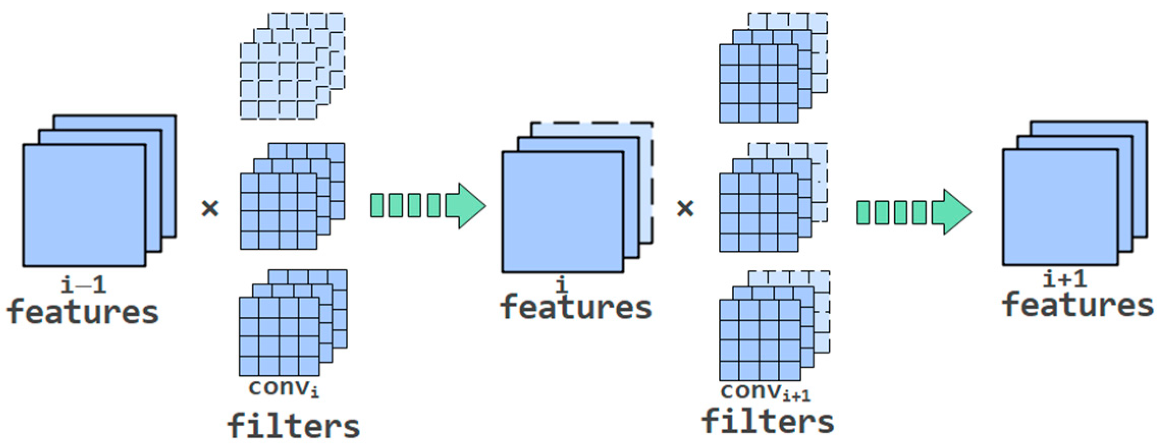
The workflow of L1-norm-based model pruning is shown in Figure 2. When the filters of the convolution layer in layer i are deleted, the number of output feature maps decreases. Consequently, the kernel of all filters in layer i + 1 should be adjusted accordingly.
In terms of the pruning process, the L1-norm based pruning method [5] provides two ideas:
  • One-shot pruning followed by retraining: this method is fast but cannot ensure that the accuracy of the pruned model is as stable as the original one.
  • Iterative pruning and retraining: the idea is to prune and retrain layer by layer, which ensures higher accuracy but needs more time. Combine-Net’s pruning process follows this idea.

2.4. Knowledge Distillation

Knowledge distillation (Figure 3) is put forward by Hinton et al. [7]. It is a widely used knowledge transfer technology in the deep learning field. First, a well-trained, robust, high-precision teacher network is needed. Its output is softened with temperature T to provide more information entropy, which extracts hidden knowledge behind its output layer. Then, a relatively small student network is trained to imitate the teacher network’s probability output distribution, obtaining a better output result.
To improve the efficiency of knowledge distillation, Haitong Li [20] used KL divergence to replace cross-entropy loss (CE) to make the final loss function become:
L K D   =   α T 2   ×   K D L i v L o s s ( Q s T , Q t T )   +   ( 1     α )   ×   C r o s s E n t r o p y ( Q s , y t r u e )
where Q s T , Q t T are the softmax probability distribution of the student network and teacher network after softening according to temperature T.

3. Methods Overview

The design principle of the work is to solve some pain points in the previous pruning algorithms, such as the inability to accurately fix the pruning rate caused by the sub-network evaluation error and the failure to repeat other pruning works caused by the lack of determining methods, etc. The authors of this work hope that Combine-Net can evaluate the performance of the sub-net more accurately, select the pruning rate of each layer more objectively, and complete faster retraining of the sub-net. Therefore, our algorithms are optimized for pruning and retraining, respectively. The following is a detailed description of these algorithms.
This section is divided into three sub-sections. The first section describes the optimization of Combine-Net in the pruning process, which is written in the Pruning Method (Section 3.1). The second section is Retraining Method (Section 3.2), using knowledge distillation to improve retraining efficiency. Finally, the General Method (Section 3.3) introduces the entire process framework of Combine-Net algorithm.

3.1. Pruning Method

This section introduces the core pruning methodologies of Combine-Net algorithm. This study, respectively, optimizes the problems of inaccurate sub-network evaluation and difficulty of determining the specific pruning rate in previous pruning work. For the sake of achieving a better effect, the Adaptive BN algorithm (Section 3.1.1) and the Kneedle algorithm (Section 3.1.2) are used to evaluate sub-networks efficiently and find the appropriate pruning rate.

3.1.1. Fast and Accurate Evaluation with Adaptive BN

Previous works often selected an indicator to reflect each neural network filter’s importance and pruned those unimportant structures. For instance, Li H et al. [5] used the L1-norm as the standard for appraising the significance of convolution kernels. Luo J et al. [21] valued the importance of each convolution kernel based on entropy. Then, both teams used an evaluation method to evaluate the effect of the sub-network after pruning to determine the final pruning plan. Specifically, this evaluation method directly assessed the sub-network quality according to its accuracy after pruning, which is called vanilla evaluation by Li B et al. [9].
However, ThiNet [10] and NetAdapt [22] used another evaluation method by first retraining the sub-net for several epochs and then checking its accuracy. Experiments showed that this method achieved better results. Hence, this work wonders whether vanilla evaluation can accurately reflect the performance of the sub-net.
To figure this problem out, the causes should be initially analyzed. Li B et al. [9] argued that the difference between these two evaluation methods is associated with the BN layer. The purpose of the BN layer’s existence is to make the neural network’s feature maps satisfy the distribution, where the mean value is 0 and the variance is 1, namely normal distribution. The BN layer prevents feature maps’ distribution from shifting with the deepening of the network, which eliminates the gradient generated by the backpropagation and accelerates the model’s convergence speed.
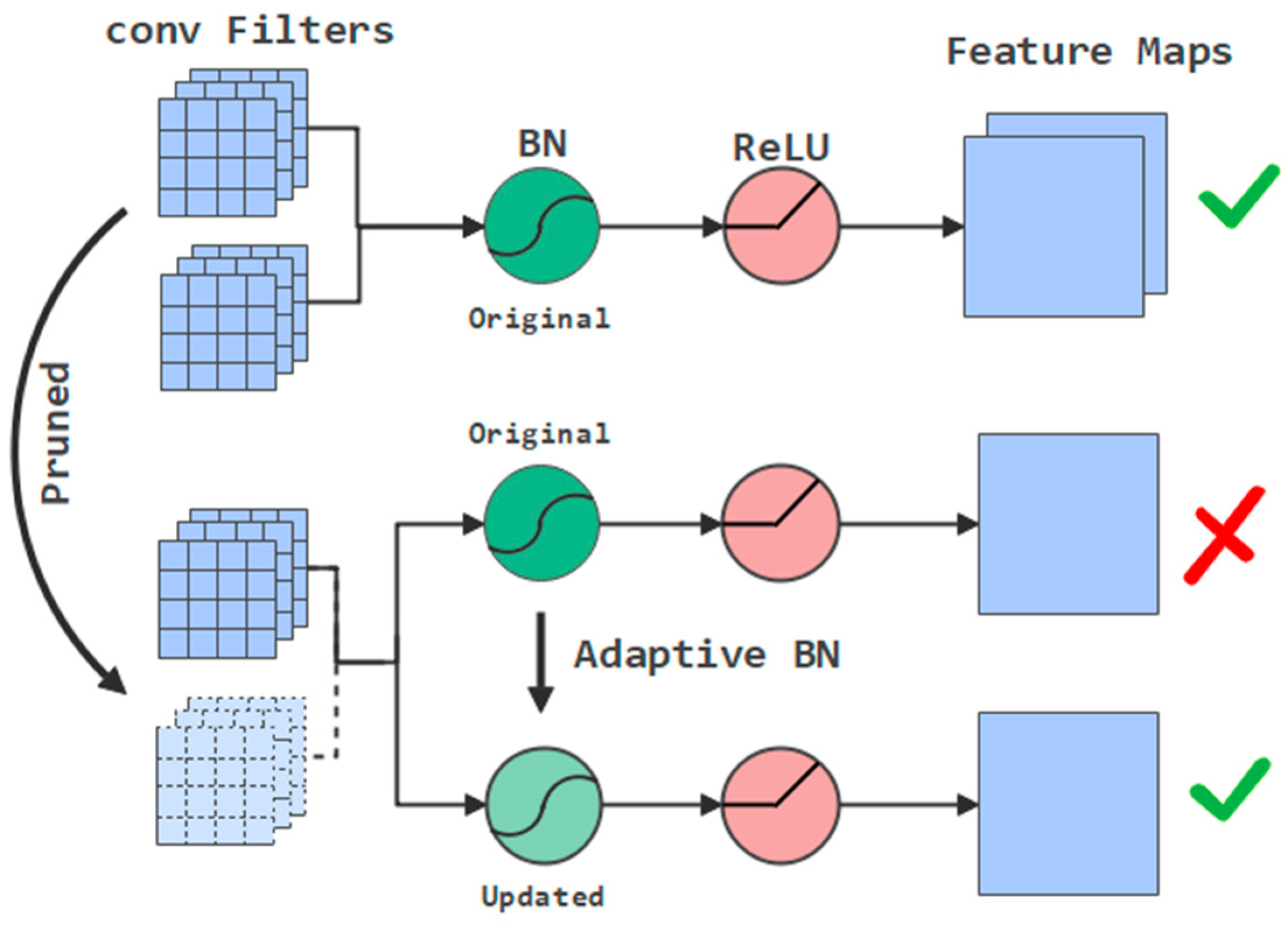
The top part in Figure 4 represents the BN layer’s correction process: the convolutional layer’s output value is corrected by Equation (1) to satisfy the normal distribution and then input to the activation layer to obtain the corresponding feature maps. The original model is:
y   =   γ x     μ σ 2   +   ϵ   +   β
where β and γ represent the trainable scale and bias terms, and ϵ is to avoid division by zero.
Parameters of the BN layer are not universal, and different convolutional layers lead to different BN layers. Nevertheless, after pruning, the sub-network structure has changed, but the BN layer has not been updated to adapt to the current network. Therefore, the mismatch between the BN layer and the sub-network explains why vanilla evaluation cannot evaluate accurately. The error generation process is shown in the middle part of Figure 4.
Hence, it is only necessary to match the BN layer structure with the pruning sub-network to eliminate errors caused by vanilla evaluation. This correction strategy is called Adaptive BN by Li B et al. [9]. The specific method is to freeze all the model parameters first. The original BN layer statistics are shown in Equation (2).
μ Β N   =   E [ x Β N ]   =   1 N n = 1 N x n ,   σ Β N 2   =   V a r [ x Β N ]   =   1 N     1 n = 1 N ( x n     μ Β N ) 2
The parameters μ and σ2 are continuously updated according to Equation (3). The evaluation process after correction is shown in the bottom part of Figure 4. The updated model is:
μ U   =   m μ U 1   +   ( 1     m ) μ Β N ,   σ U 2   =   σ U 1 2   +   ( 1     m ) σ Β N 2
where m is the momentum coefficient and subscript U refers to the number of updated iterations. In a typical updating pipeline, if the total number of updated iterations is U, the corresponding μ and σ2   are   μ U and σ U 2 , used in the testing phase. These two items are called full-size model BN statistics.
Adaptive BN only updates the BN layer parameters, while the retraining method used by ThiNet [10] and NetAdapt [22] updates all the parameters of the model. Compared with the latter, Adaptive BN is faster. Li B et al. [9] have shown that the 100-epoch update time is still at the second level. To sum up, Adaptive BN evaluates the sub-network performance quickly and accurately. Therefore, Combine-Net uses it to replace vanilla evaluation.

3.1.2. Determination of the Appropriate Pruning Rate by Kneedle

Pruning rates are the specific content of pruning algorithms. No matter what evaluation criteria are selected, only when the pruning rate of each layer is determined can this layer be pruned. Generally speaking, the higher the sensitivity of the layer, the lower the acceptable pruning rate. Based on this, Li H et al. [5] put forward their pruning plan. As shown in Table 1, taking VGG16 as an example, they chose not to prune the 2–7 convolution layers with low sensitivity. For the 8–13 convolution layer with relatively high sensitivity, they adopted 50% pruning rates. Their pruning scheme was accumulated through multiple experiments, so this method is termed “empirical.”
It is unreasonable to confirm the pruning rate empirically. The first reason is that, to obtain the empirical pruning rate in neural networks with different structures, a large amount of experimental data is fundamental. This large-scale experiment will consume many workforces and material resources in analyzing and comparing the data. Second, even for networks with the same structure, different datasets often lead to different pruning rates. Combine-Net seeks out a better determining method to solve this problem. Thus, this work introduces the concept of the knee point [23] in mathematics to determine the appropriate pruning rate.
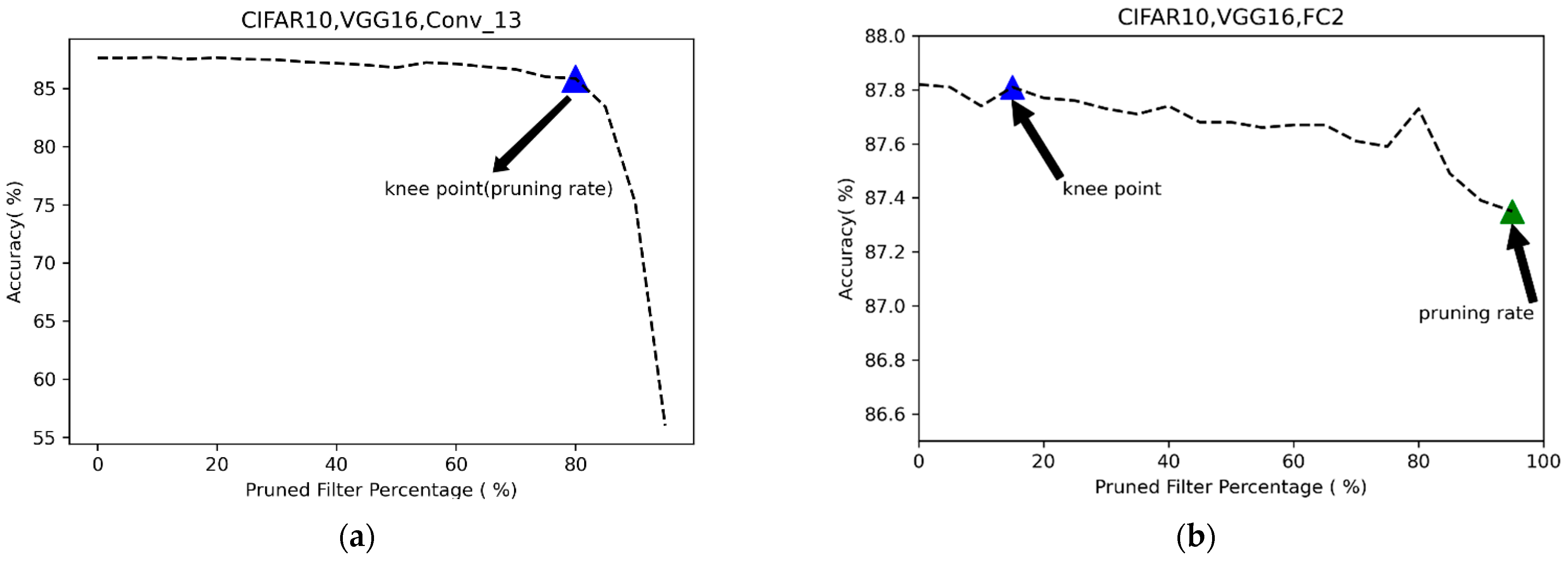
Some points like this often exist in the real world: once beyond them, the additional cost no longer receives the corresponding performance benefits. These points are called Knee Points. Planners are more willing to choose these points to best balance investment and return. In determining the pruning rate, the same requirement should be applied: obtaining a higher pruning rate while ensuring accuracy. Accordingly, a reasonable pruning rate can be decided by searching for the Knee Point during pruning. The Knee Point’s position, which means the appropriate pruning rate, is calculated by analyzing the pruning curve. The calculating method is called the Kneedle algorithm by Satopaa V et al. [23]. This work tested the Kneedle algorithm on the 13th convolutional layer of VGG16. It can be seen from Figure 5 that the algorithm determines the position of the knee points very well, which can be used as the pruning rate of this layer.

3.1.3. How to Confirm the Knee Point

The Kneedle algorithm is summarized in this section. The core idea of the Kneedle algorithm is to find the position where the curvature of the pruning rate–accuracy rate curve changes the most, which can achieve the best balance between the two variables. The pipeline of the Kneedle algorithm is shown as the algorithm flow in Algorithm 1.
Algorithm 1 Using the Kneedle Algorithm to Determine the Pruning Rate.
1: Input: The number of neural network’s layers: Lay_Num;
    Pre pruning rate of each layer r%;
    The accuracy rate corresponding to the pre pruning rate: acc%;
2: Output: True pruning rate of each layer: R%;
3: for i = 1 to Lay_Num do
4:    # Smooth the curve.
5:    Smooth (ri, acci);
6:    # Calculate the position of the knee point.
7:    Ri = Calculate_Knee_Point (ri, acci);
8:    # Verify the rationality of the knee point.
9:    Ri = Vertify_Knee_Point (ri, acci);
10: end for
11: return R;
First of all, the algorithm needs to preprocess the original curve. The original pruning rate–accuracy rate curve is not smooth enough. In this case, a lot of turbulence may lead to algorithm failure. Combine-Net uses a smoothing spline to preserve the shape of the original curve as much as possible.
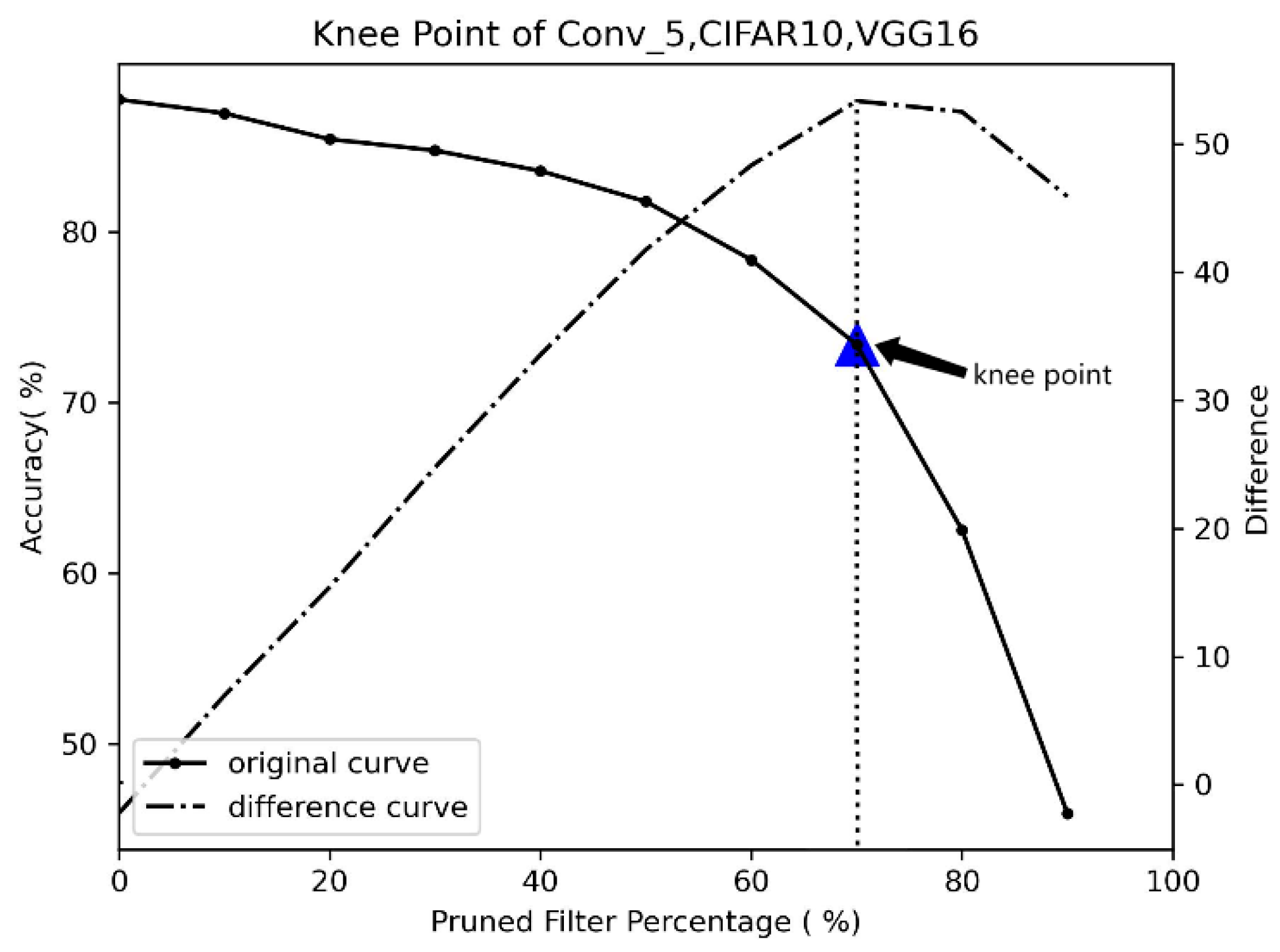
Next, let D d represent the set of differences between pruning rate ( r % ) and accuracy rate ( a c c % ), that is, the set of points ( r , a c c     ( 100 %     r ) ) , as shown in the difference curve in Figure 6. The algorithm does not care about the initial values of r and a c c , because the goal is to find out when the curve changes its trend. Then, find out the point with the largest value in the difference curve. As shown in Figure 6, the r of this point is the r of the knee point in the original curve. In this way, the knee point can be determined.
Finally, some methods must be used to verify the rationality of the knee point because a leak exists in the Kneedle algorithm. Even if a high rate for layers with low sensitivity is used, the sub-network still maintains a high accuracy rate. In this case, the Kneedle algorithm often cannot provide the appropriate pruning rate. As a result, this research offers a solution in that setting a tolerable threshold of the precision dropping rate and taking the maximum pruning rate satisfying the threshold. As shown in Figure 5b, the second full connection layer of VGG16 was pruned with a series of rates, and its sub-networks’ accuracy remained in a reasonable range. However, the rate given by the Kneedle algorithm is indeed 15%. For this case, a tolerable precision dropping threshold of 0.5% was set. When the pruning rate reached the maximum (95%), it still satisfied the threshold. As a result, the pruning rate here was indeed deemed as 95%.
The advantages of using the Kneedle algorithm to determine the pruning rate are significant:
  • The algorithm is relatively more objective and does not require subjective experience as a basis for judgment.
  • The algorithm determines the pruning rate faster and does not require experimentation to accumulate expertise.
  • The algorithm is highly applicable and suitable for determining the pruning rate of any model.
  • This algorithm meets the needs of different precisions. The pruning rate is more accurate when the data are denser.

3.2. Retraining Method

Since the widely used pruning process was proposed by Han et al. [6], retraining after pruning has been deeply rooted in the hearts of the researchers. However, how to carry out effective retraining is a problem worthy of discussion. Only one retraining after all the pruning works will lead to a significant reduction in models’ accuracy. Pruning and retraining layer by layer will lead to excessive time consumption. Therefore, Combine-Net hopes to find a better way to improve the efficiency of retraining.
Luo JH et al. [10] have already proposed their solution: after pruning a layer, a few iterations are used to restore partial performance. When all the layers are pruned, more iterations will be used to restore the overall accuracy. Combine-Net’s retraining method continues this idea. However, the efficiency of ordinary fine-tuning is still low. Considering that knowledge distillation can transfer the information in the original network very well, so it is introduced to obtain a highly efficient retraining method.
In the retraining of using knowledge distillation, the original unpruned network works as the teacher network, which has the advantages of robustness and high accuracy. The pruned sub-network is viewed as the student network to learn from the teacher. After pruning, some hidden dark knowledge in the original model, which is not well utilized, disappears with the pruned filters. Combine-Net extracts this part of knowledge from the original model through knowledge distillation as another learning source of the sub-networks’ retraining. Knowledge distillation makes full use of the information hidden in the original model, provides more learning objects for the sub-network, thus improving the efficiency of retraining.
Chen L et al. [24] also put forward the idea of using knowledge distillation. Compared with theirs, the Combine-Net algorithm is based on the sub-net after structural pruning, which has more strong universality and does not need exceptional hardware support. As a result, the research has more reference significance.

3.3. General Method

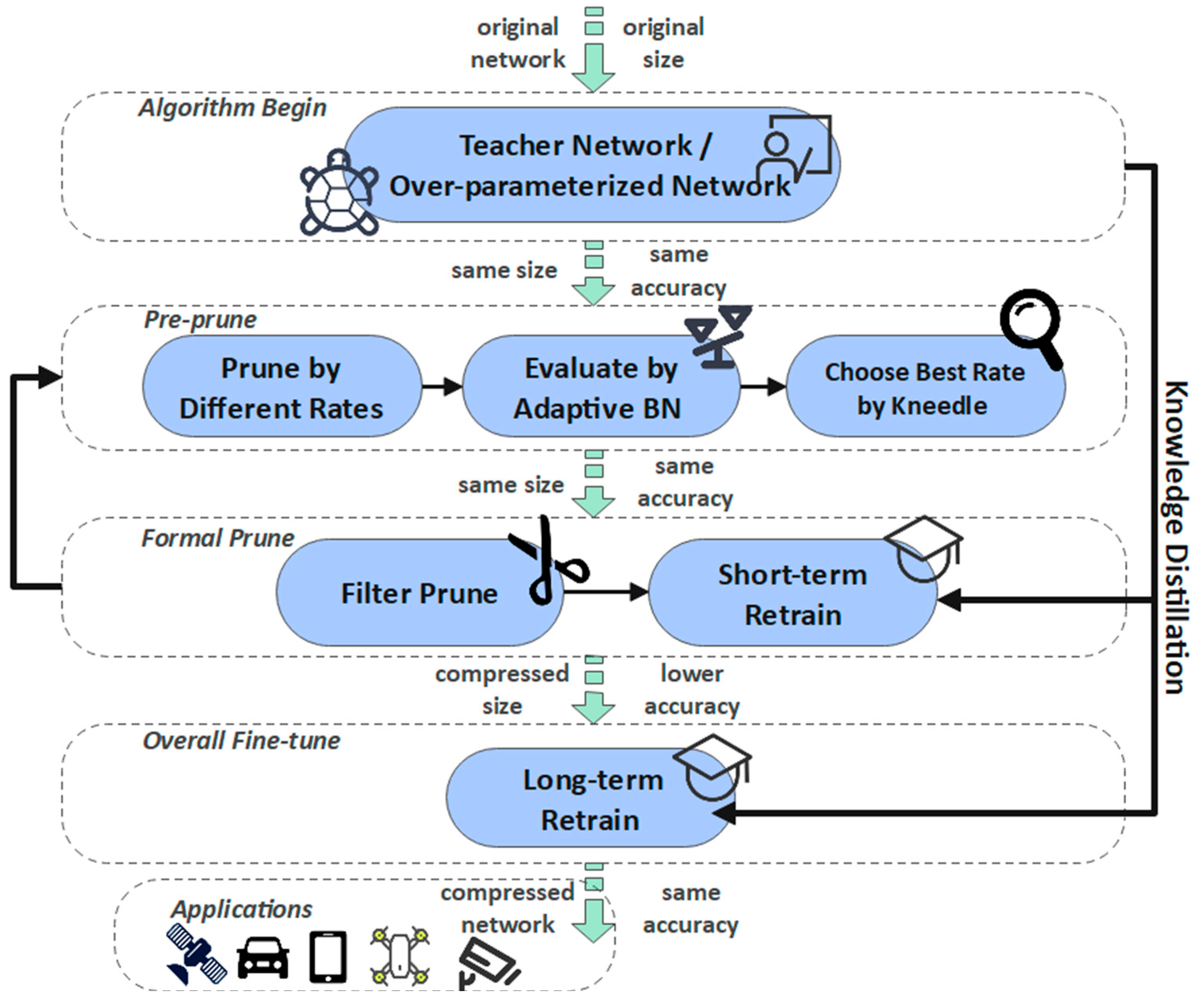
This part summarizes the three improved algorithms described above and proposes a new proved pruning algorithm (Figure 7). The algorithm’s process is similar to that offered by Han et al. [6], which is repeating pruning and fine-tuning to satisfy the accuracy requirements of sub-networks. The concrete process is as follows:
  • A pre-trained and over-parameterized network needs to be obtained first, as not only a pruning object but also a teacher network, to guide the retraining of the sub-network.
  • Start pruning layer by layer: the convolution layers or full connection layers that need to be pruned should be pre-cut according to different proportions. After that, evaluate these sub-nets fine or not by Adaptive BN. Finally, the best pruning rate is determined by the Kneedle algorithm. Then, the formal pruning is carried out.
  • After each layer of pruning, the precision is slightly restored through a few rounds of retraining. The concrete method of retraining is to use knowledge distillation to distill dark knowledge from the pre-training network to guide the sub-network learning. Being layer-by-layer pruned and retrained, the parameterized model is compressed into a compact sub-network. Finally, restore the global accuracy of the model by multiple rounds of retraining.

4. Experiment

All the algorithms of this work were conducted by the standard PyTorch 1.7.1 library. The CUDA version was 10.1 with NVIDIA GeForce RTX 2080Ti GPU and Intel Core i3-9100F CPU @ 3.60GHz. This experiment mainly verified some modules of the algorithm on the VGG16. To test the effect of the whole algorithm, this work also experimented on the residual network ResNet32 and ResNet50, mainly using CIFAR10 and CIFAR100.
The datasets we used were standard CIFAR10 and CIFAR100. There are 60,000 color images in CIFAR10, which are divided into ten categories. Each category contains 6000 images, of which 5000 images were used for training, and another 1000 for testing. Similarly, the CIFAR100 dataset has 100 classes, each containing 600 images, with 500 training images and 100 test images.
Furthermore, our experiment did not use any particular parameter tuning method, and all the models were obtained through fixed epochs of iteration under a fixed learning rate. On the retraining process, the optimizer was Adam, whose learning rate was initialized as 1 × 10⁻⁴. Some hyperparameters used in knowledge distillation were T initialized as 5.0 and α initialized as 0.7.
In evaluating the model compression effect, M was the unit we used to measure the parameter amount. GMacs means Giga multiply add calculation per second, which was the standard to measure the amount of calculation. Top-N accuracy refers to the probability that one of the first n answers given by the neural network is correct. We used Top-1 Acc. and Top-5 Acc. to estimate networks’ accuracy.
The experimental code has been open source, and readers can find it in the Supplementary Materials.

4.1. Proper Pruning Rate Improves Algorithm Efficiency

4.1.1. Significant Effect of Adaptive BN in Pruning Evaluation

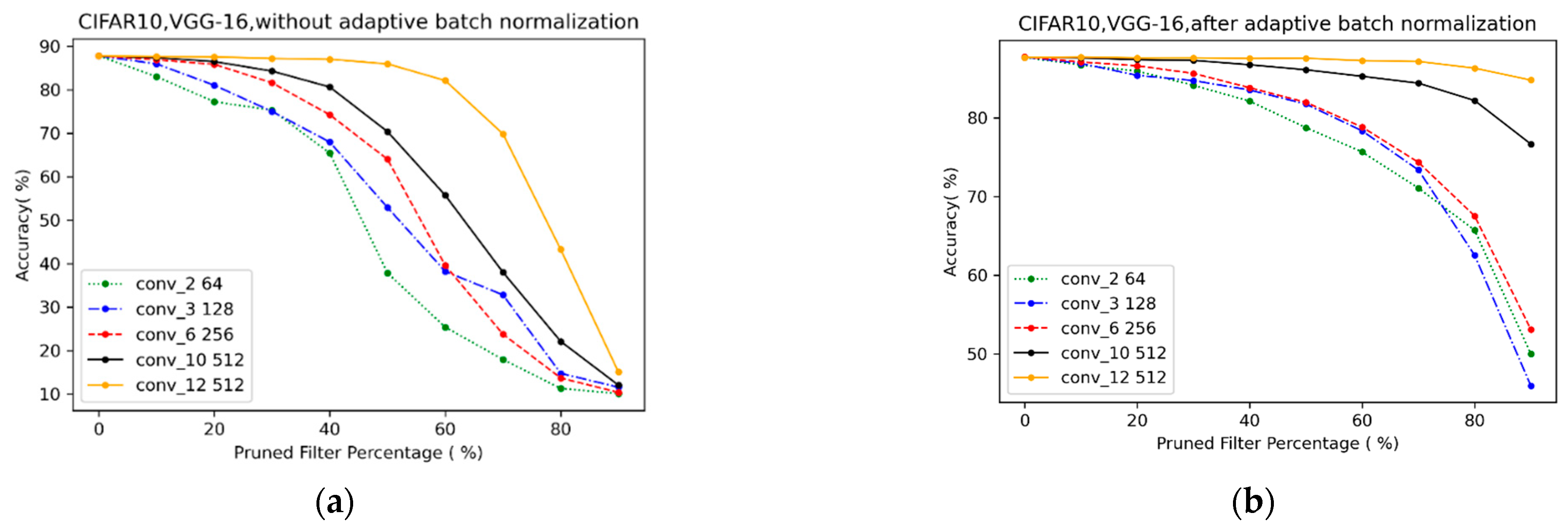
To verify Adaptive BN’s reliability, this work repeated the sensitivity experiment by Li H et al. [5]. The experiment pruned five representative convolution layers of VGG16 on CIFAR10 with different pruning rates and assessed the performance of the sub-nets by two evaluation methods: one is the vanilla evaluation, which is widely used in past works to evaluate the networks’ accuracy directly. The other is to assess after Adaptive BN. The result is shown in Figure 8.
Figure 8a is the effect of vanilla evaluation. Compared with it, the accuracy adjusted by Adaptive BN in Figure 8b better reflects the network’s actual performance. The effect of promotion is reflected in the less volatile curve and the smooth accuracy decline in Figure 8b, indicating the gradual network performance deterioration during pruning. Moreover, when the pruning rate is 95%, most convolution layers’ accuracy increases from 10% (Figure 8a) to about 50% (Figure 8b); the accuracy is significantly improved. Therefore, the Adaptive BN can effectively obtain the sub-networks’ factual efficiency.

4.1.2. Choose the Best Pruning Rate by Kneedle

This work verified whether the Kneedle algorithm can give a reasonable pruning rate by using VGG16 on the CIFAR10. The experiment independently pruned the 13 convolution layers of VGG16 by using the pruning rate determined empirically [5] and the rate given by the Kneedle algorithm separately. It then compared the variation in the accuracy of the sub-networks after slight retraining. VGG16 used in [5] contains only two full connection layers, lacking one layer compared with the general VGG16, which makes the comparison of the pruning of the fully connected layer in our experiment meaningless. The experiment was repeated five times, recording each layer’s pruning rate provided by the Kneedle algorithm and the mean value, and the standard deviation of Top-1 accuracy after pruning (see Table 1).
From the comparison of the results in Table 1, the Kneedle algorithm is capable of providing a proper pruning rate. The Kneedle algorithm can design suitable pruning rates for different convolution layers compared with empirical methods. For convolution layers with high sensitivity, such as Conv_1, the Kneedle algorithm gave relatively small pruning rates (20%); as for layers with low sensitivity such as Conv_13, a large pruning rate (80%) was provided. Moreover, after slight retraining, the accuracy of the sub-network was restored to a relatively good position, and even the maximum Top-1 accuracy reduction was no more than 3%.
In addition, compared with the pruning rate determined empirically based on Li H et al. [5], the pruning rate determined by the Kneedle algorithm is not fixed: different convolution layers have different pruning rates. However, for layers with the same number of convolution kernels, a similar pruning rate also occurs. For example, for Conv_3 and Conv_4 with 128 convolution kernels, the algorithm gave the same pruning rate (60%), for Conv_5, Conv_6, and Conv_7 with 256 convolution kernels; the algorithm provided similar pruning rates close to 65% and for the layers with 512 convolution kernels, the pruning rate was about 75%.
Consequently, Kneedle algorithm can be applied to obtain a proper pruning rate.

4.2. Efficient Retraining with Knowledge Distillation

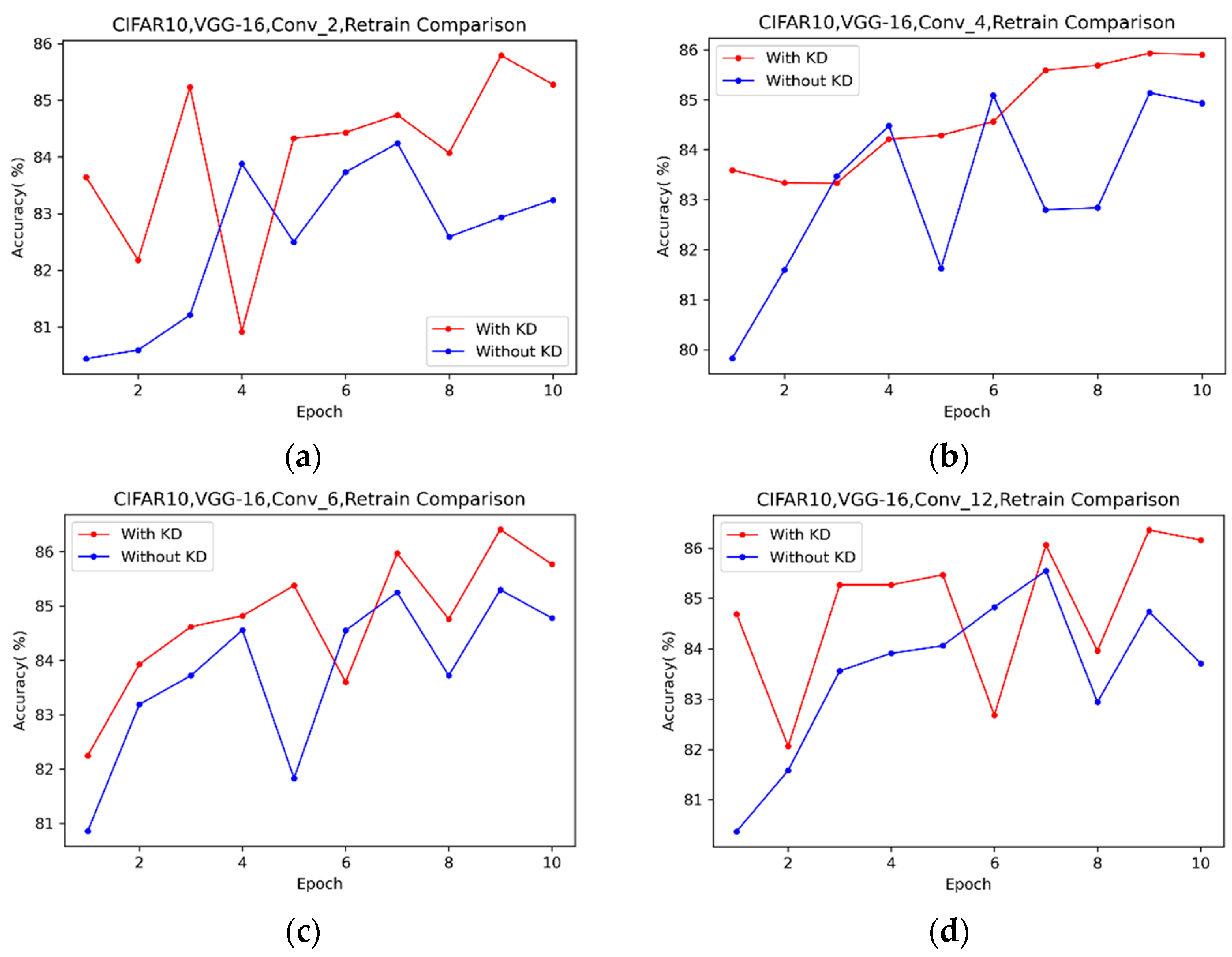
The experiment assessed its short-term and long-term effects independently to verify the significance of knowledge distillation.

4.2.1. Short-Term Effects

Short-term retraining between layers is used to recover the general accuracy of the sub-networks roughly. This part of the experiment used two methods—retraining with knowledge distillation and without knowledge distillation—to prune Conv_2, Conv_4, Conv_6, and Conv_12 of the VGG16 model. Each method iterated ten epochs, respectively, investigating the effects of knowledge distillation (see Figure 9). In the different sizes of VGG16′s layers, the accuracy curve of using knowledge distillation was 1–2 percentage points above the status quo approach. Consequently, knowledge distillation restored more accuracy through fewer iterations.

4.2.2. Long-Term Effects

Moreover, it is necessary to consider the effect of knowledge distillation in restoring the condition’s overall performance with long-term iteration. After pruning the model, this work iterated 120 epochs with these two retraining methods above—training results are shown in Figure 10. The training method of knowledge distillation was still better than the regular training in more iterations. It recovered accuracy faster under the same iteration round and achieved higher accuracy at last, which was 0.5 percentage more elevated than the result of regular retraining.
In addition, it can be seen from Figure 10 that, whether knowledge distillation is applied or not, the accuracy of the two retraining methods is still rising when the iteration epoch is 120. In other words, the accuracy does not decrease with the training, which is contrary to the phenomenon of overlearning. This work sets all the epochs of retraining as 120, which is relatively less, and did not pursue high accuracy deliberately. Therefore, there is no significant overlearning problem in this work.

4.3. Evaluate the Effect of Combine-Net’s Improvements

4.3.1. VGG16 on CIFAR 10

The VGG16 on the CIFAR10 is an over-parameterized network containing 13 convolution layers and three full connection layers. This initially trained model had a Top-1 accuracy of 87.82% and a Top-5 accuracy of 99.55%, as shown in Table 2. The experiment tested the complete pruning algorithm on VGG16. The final pruning result is shown in Table 3, and performance of the model after retraining is shown in Table 2.
Comparing Table 3 with Table 1, the pruning rates of convolutional layers in Table 3 are relatively lower. However, the algorithm still provided an appropriate pruning rate for each layer of the neural network to ensure that its accuracy will not decrease significantly after retraining. The data in Table 2 show that the accuracy of the pruned sub-network was recovered to a great degree after the overall retraining, even better than the original over-parameterized network, and its parameter amount was compressed by more than 90%. The calculation amount was compressed by more than 80%. The experiment also pruned the convolution layer of VGG16 according to the pruning rate given by Li h et al.’s work [5], and the results are shown in Table 2. Compared with their work [5]—parameter amount was 34%, the calculation amount was 26%, and the effect of the algorithm in this study was obviously better.

4.3.2. ResNet34 on CIFAR10

To verify Combine-Net’s performance on residual networks, experiments on ResNet34 were also conducted. ResNet34, an intense residual network, has higher accuracy but also extends the neutral network depth too deep. For the layer-by-layer pruning algorithm, it means longer pruning time. Therefore, when dealing with this kind of network, only the more redundant blocks are tended to be pruned. In our experiment, we only pruned basic blocks where the numbers of filters were 256 and 512—the last nine basic blocks. The final pruning effect is shown in Table 2.
As Table 2 shows, the algorithm also had a good effect on ResNet34. The decrease in Top1 accuracy was less than 0.5%, the number of parameters was compressed by more than 90%, the amount of calculation was compressed by more than 50%, and the model size was reduced by nearly 75 MB. However, how to overcome the time cost of layer-by-layer pruning still needs further research.

4.3.3. ResNet50 on CIFAR100

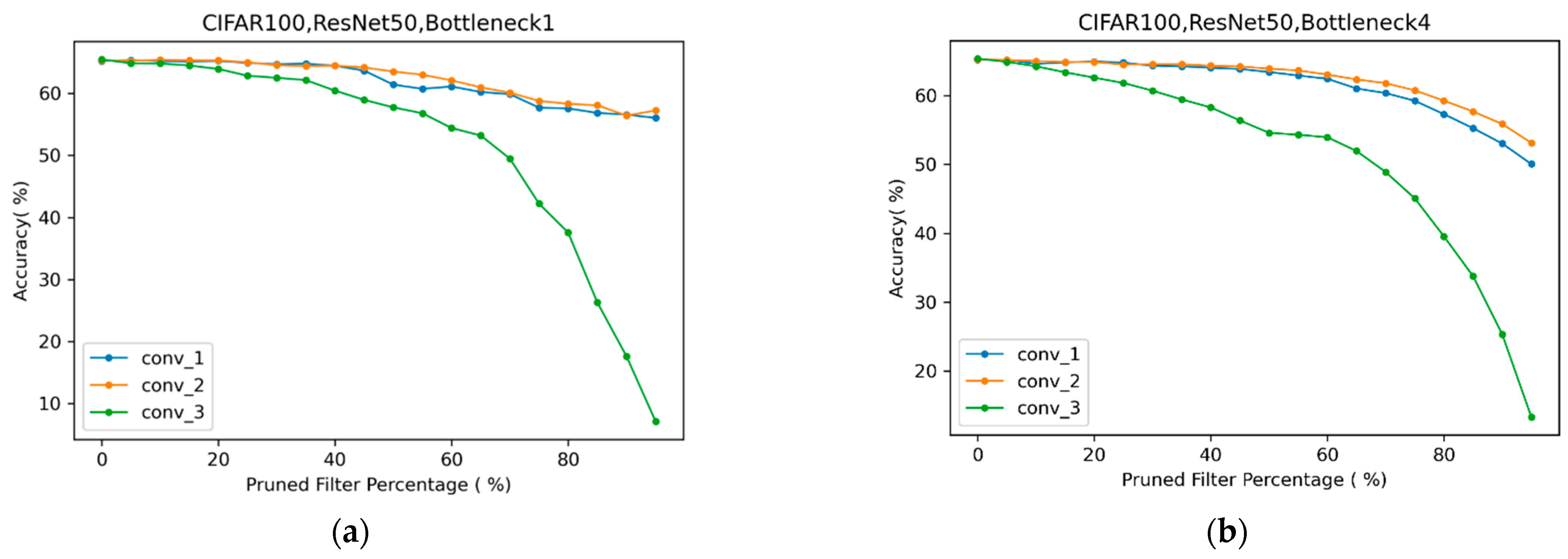
ResNet50 on CIFAR100 were trained and pruned to prove the algorithm’s effect on more complex datasets. The concrete pruning method was consistent with that of ResNet34, which means, only the last nine blocks were pruned. In addition, the sensitivity of three convolutional layers in the first and forth bottleneck of ResNet50 is shown in Figure 11. As the third layer in ResNet50’s bottleneck was too sensitive to be pruned and the accuracy could not recover well after retraining, so the third layer was left unpruned.
The performance of the sub-network after pruning is shown in Table 2. The compression of the amount of parameters and calculations of the model had a specific decrease compared with VGG16 and ResNet34. This is because, for some complex data sets such as CIFAR100, the neural network model needs to learn more knowledge, which leads to the increase in the effective utilization rate of the model, and the decrease in redundancy and pruning rate. However, the algorithm still compressed the model effectively, and the parameter and calculation amount had been significantly reduced.

5. Discussion

This work attempts to create a pruning algorithm with higher accuracy and more objectivity. Experiments on different neural networks verified the reliability of Combine-Net, which confirmed the outstanding role of Adaptive BN operation, Kneedle, and retraining combined with knowledge distillation. Compared with some essential work, the pruning method used by Li B et al. [9] is to find the optimal sub-network through a large amount of random pruning, which consumes too much pruning time. In contrast, this work prunes by L1-norm, making it faster to find a suitable sub-network. Furthermore, based on the work of Li H et al. [5], this work improves the method of determining the pruning rate, increasing the objectivity and accuracy of the algorithm, and combines knowledge distillation with retraining, shortening the retraining time and improving the accuracy of the sub-network at the same time.
Although this work has revealed some critical discoveries, many places can be further improved. First, the knowledge distillation method used in retraining is not immutable and frozen. With the continuous development of this technology, better knowledge distillation methods will emerge in an endless stream. Moreover, Chen L et al. [24] noted that different knowledge distillation methods suited other neural network structures. Therefore, further research is needed to promote a deeper integration of retraining and knowledge distillation.
Second, for deep convolutional neural networks, especially intense residual networks such as ResNet101 and ResNet152, layer-by-layer pruning means extremely long pruning time, which has been a problem since the method was proposed by Li H et al. [5]. To overcome this challenge, the retraining method of Combine-Net can recover more accuracy in fewer epochs, thus shortening the time of retraining. However, the time consumed in determining the pruning rate cannot be ignored. In this experiment, each neural network layer was pruned in the range from 0% to 95% to find the best pruning rate. As a result, reducing the search range of pruning rate is proposed to shorten the time consumption. Zhuang L et al. [25] emphasized the importance of model structure. Therefore, it can be conjectured that models with the same design may have a similar pruning rate. Of course, the impact of data sets on pruning rate cannot be denied, but a recommended pruning rate for each model structure can still be chosen through a large number of experiments. In this way, during the subsequent pruning process, the search range of pruning rate can be reduced to near the recommended rate, which reduces the time cost.
Finally, the method of selecting the optimal pruning rate layer by layer is essentially a greedy algorithm. Therefore, it is impossible to evaluate whether the rates it determined are of globally optimal accuracy. This work also tried other pruning rate determination methods, such as dynamic programming algorithms and heuristic algorithms. However, because these algorithms need to compute more states to obtain relatively accurate results, their running time is unacceptable. This is the reason why Combine-Net chose to combine the greedy algorithm with the Kneedle algorithm. In future research, this work will conduct further experiments to verify whether the algorithm can give the optimal global solution and find some updated neural network methods to obtain more effective model pruning.

6. Conclusions

In this work, we were committed to obtaining an accurate, objective, and efficient neural network pruning algorithm to compress redundant neural networks. Our work introduced the Adaptive BN to correct the BN layer of the sub-network after pruning, which increased the accuracy of the evaluation. Furthermore, the work used the Kneedle algorithm to give an objective and appropriate pruning rate. Finally, we applied the knowledge distillation method to restore the model’s accuracy, improving retraining efficiency. We proposed Combine-Net based on the above and carried out experimental verification on different neural network models and datasets. The results showed that the algorithm achieved significant compression of neural network parameters and calculations in various situations without accuracy loss.
Future work to solve the tricky problem of excessively long pruning time includes:
  • Analyzing the relationship between model structure and pruning rate.
  • Providing recommended pruning rates for different model structures.
  • Looking for a method to replace the greedy algorithm of layer-by-layer pruning.
  • Extending the algorithm to unstructured pruning and verifying Combine-Net’s universality and robustness.

Supplementary Materials

The following are available online at https://github.com/Chicory-ggg/Combine-Net, accessed on 23 June 2020. Source code and the pruned models are accessible to open-source community.

Author Contributions

Methodology, G.L. and J.W.; software, G.L.; formal analysis, G.L. and J.W.; resources, W.Z.; data curation, G.L.; writing—original draft preparation, G.L. and J.W.; writing—review and editing, W.Z. and G.L.; visualization, J.W.; project administration, W.Z. All authors have read and agreed to the published version of the manuscript.

Funding

This research received no external funding.

Institutional Review Board Statement

Not applicable.

Informed Consent Statement

Not applicable.

Conflicts of Interest

The authors declare no conflict of interest.

References

  1. Amato, G.; Carrara, F.; Falchi, F.; Gennaro, C.; Meghini, C.; Vairo, C. Deep learning for decentralized parking lot occupancy detection. Expert Syst. Appl. 2017, 72, 327–334. [Google Scholar] [CrossRef]
  2. Li, Y.; Chen, F.; Sun, Z.; Ji, J.; Jia, W.; Wang, Z. A Smart Binaural Hearing Aid Architecture Leveraging a Smartphone APP with Deep-Learning Speech Enhancement. IEEE Access 2020, 8, 56798–56810. [Google Scholar] [CrossRef]
  3. Xu, C.; Mao, Y. An Improved Traffic Congestion Monitoring System Based on Federated Learning. Information 2020, 11, 365. [Google Scholar] [CrossRef]
  4. Sandler, M.; Howard, A.; Zhu, M.; Zhmoginov, A.; Chen, L.C. Mobilenetv2: Inverted residuals and linear bottlenecks. In Proceedings of the IEEE Conference on Computer Vision and Pattern Recognition, Salt Lake City, UT, USA, 18–23 June 2018; pp. 4510–4520. [Google Scholar]
  5. Li, H.; Kadav, A.; Durdanovic, I.; Samet, H.; Graf, H.P. Pruning filters for efficient convnets. arXiv 2016, arXiv:1608.08710. [Google Scholar]
  6. Han, S.; Mao, H.; Dally, W.J. Deep compression: Compressing deep neural networks with pruning, trained quantization and huffman coding. arXiv 2015, arXiv:1510.00149. [Google Scholar]
  7. Hinton, G.; Vinyals, O.; Dean, J. Distilling the knowledge in a neural network. arXiv 2015, arXiv:1503.02531. [Google Scholar]
  8. Hu, H.; Peng, R.; Tai, Y.W.; Tang, C.K. Network trimming: A data-driven neuron pruning approach towards efficient deep architectures. arXiv 2016, arXiv:1607.03250. [Google Scholar]
  9. Li, B.; Wu, B.; Su, J.; Wang, G. Eagleeye: Fast sub-net evaluation for efficient neural network pruning. In Proceedings of the 16th European Conference on Computer Vision, Glasgow, UK, 23–28 August 2020; Springer International Publishing: Cham, Switzerland, 2020; pp. 639–654. [Google Scholar]
  10. Luo, J.H.; Wu, J.; Lin, W. Thinet: A filter level pruning method for deep neural network compression. In Proceedings of the IEEE International Conference on Computer Vision, Venice, Italy, 22–29 October 2017; pp. 5058–5066. [Google Scholar]
  11. Denil, M.; Shakibi, B.; Dinh, L.; Ranzato, M.A.; De Freitas, N. Predicting parameters in deep learning. arXiv 2013, arXiv:1306.0543. [Google Scholar]
  12. Iandola, F.N.; Han, S.; Moskewicz, M.W.; Ashraf, K.; Dally, W.J.; Keutzer, K. SqueezeNet: AlexNet-level accuracy with 50x fewer parameters and <0.5 MB model size. arXiv 2016, arXiv:1602.07360. [Google Scholar]
  13. Howard, A.G.; Zhu, M.; Chen, B.; Kalenichenko, D.; Wang, W.; Weyand, T.; Adam, H. Mobilenets: Efficient convolutional neural networks for mobile vision applications. arXiv 2017, arXiv:1704.04861. [Google Scholar]
  14. Zhang, X.; Zhou, X.; Lin, M.; Sun, J. Shufflenet: An extremely efficient convolutional neural network for mobile devices. In Proceedings of the IEEE Conference on Computer Vision and Pattern Recognition, Salt Lake City, UT, USA, 18–23 June 2018; pp. 6848–6856. [Google Scholar]
  15. Xie, S.; Girshick, R.; Dollár, P.; Tu, Z.; He, K. Aggregated residual transformations for deep neural networks. In Proceedings of the 2017 IEEE Conference on Computer Vision and Pattern Recognition (CVPR), Honolulu, HI, USA, 21–26 July 2017. [Google Scholar]
  16. Chollet, F. Xception: Deep learning with depthwise separable convolutions. In Proceedings of the IEEE Conference on Computer Vision and Pattern Recognition, Honolulu, HI, USA, 21–26 July 2017; pp. 1251–1258. [Google Scholar]
  17. Courbariaux, M.; Bengio, Y.; David, J.P. Binaryconnect: Training deep neural networks with binary weights during propagations. arXiv 2015, arXiv:1511.00363. [Google Scholar]
  18. Fang, B.; Zeng, X.; Zhang, M. Nestdnn: Resource-aware multi-tenant on-device deep learning for continuous mobile vision. In Proceedings of the 24th Annual International Conference on Mobile Computing and Networking, New Delhi, India, 29 October–2 November 2018; pp. 115–127. [Google Scholar]
  19. He, Y.; Kang, G.; Dong, X.; Fu, Y.; Yang, Y. Soft filter pruning for accelerating deep convolutional neural networks. arXiv 2018, arXiv:1808.06866. [Google Scholar]
  20. Li, H. Exploring Knowledge Distillation of Deep Neural Nets for Efficient Hardware Solutions. CS230 Report. 2018. Available online: https://github.com/peterliht/knowledge-distillation-pytorch (accessed on 23 June 2020).
  21. Luo, J.H.; Wu, J. An entropy-based pruning method for cnn compression. arXiv 2017, arXiv:1706.05791. [Google Scholar]
  22. Yang, T.J.; Howard, A.; Chen, B.; Zhang, X.; Go, A.; Sandler, M.; Adam, H. Netadapt: Platform-aware neural network adaptation for mobile applications. In Proceedings of the European Conference on Computer Vision (ECCV), Munich, Germany, 8–14 September 2018; pp. 285–300. [Google Scholar]
  23. Satopaa, V.; Albrecht, J.; Irwin, D.; Raghavan, B. Finding a “kneedle” in a haystack: Detecting knee points in system behavior. In Proceedings of the 2011 31st International Conference on Distributed Computing Systems Workshops, Minneapolis, MN, USA, 20–24 June 2011; pp. 166–171. [Google Scholar]
  24. Chen, L.; Chen, Y.; Xi, J.; Le, X. Knowledge from the original network: Restore a better pruned network with knowledge distillation. Complex Intell. Syst. 2021, 1–10. [Google Scholar]
  25. Liu, Z.; Sun, M.; Zhou, T.; Huang, G.; Darrell, T. Rethinking the value of network pruning. arXiv 2018, arXiv:1810.05270. [Google Scholar]
Figure 1. Illustration of unstructured pruning and structured pruning. (a) Unstructured pruning, where synapses—unimportant connections, can be pruned in order to sparse the network. Neurons can also be pruned to achieve the same purpose. (b) A typical structured pruning that prunes the filters. Channels of the generated feature maps are reduced accordingly.
Information 12 00264 g001
Figure 2. The workflow of L1-norm-based model pruning, in which the light-colored structure should be pruned. If one filter in conv i is pruned, its corresponding feature map in layer i will be removed. Then, the filters in conv i + 1 will be adjusted to fit structural changes.
Information 12 00264 g002
Figure 3. The main idea of knowledge distillation. The label of the input image is cat; the probability is expressed as {0, 1, 0}. After the inference of teacher network and student network, the algorithm outputs classification results q and q’, so that the image is declared as a cat. However, this image also shows some dog traits, which is not shown obviously in q and q’. After softening the teacher network, the dark knowledge appears. The classification result is q’’, which provides more dark knowledge. Training the student network with the teacher network makes the student network more accurate on the basis of the teacher network’s characteristics.
Information 12 00264 g003
Figure 4. The dark green circle represents the original BN layer, which proceeds with the unpruned model. However, after being pruned, the structure of model has changed, and original BN layer cannot adapt the new model, whose results have poor accuracy. If the BN layer (marked by the light green circle) is updated by the Adaptive BN [9], the resulting accuracy will be better.
Information 12 00264 g004
Figure 5. The blue triangles in (a,b) are Knee points, which refer to the curve’s change to a sharp decline from the horizontal. (a) Shows that the Kneedle algorithm can find the pruning rate well in the general convolution layer. (b) Shows that, for some insensitive fully connection layers, the accuracy decreases little, and Kneedle algorithm cannot give an appropriate pruning rate; the green triangle is the maximum pruning rate that meets the threshold.
Information 12 00264 g005
Figure 6. The process of determining the knee point is shown in this figure. First, calculate the difference curve according to the original curve. Then, the knee point can be found by calculating the maximum value of the difference curve, because of the same abscissa.
Information 12 00264 g006
Figure 7. The workflow of Combine-Net.
Information 12 00264 g007
Figure 8. Comparison of two evaluation methods. (a) Demonstrates the effect of vanilla evaluation. (b) Shows the evaluation effect after incorporating Adaptive BN.
Information 12 00264 g008
Figure 9. Short-term training results. This figure shows the differences in the accuracy recovery speed of VGG16 on CIFAR10’s various convolution layers in short-term retraining. The convolutional layers pruned in subfigures (ad) are all from the same VGG16 but with different filter numbers.
Information 12 00264 g009
Figure 10. Long-term training results.
Information 12 00264 g010
Figure 11. The accuracy of different pruning percentages. The third convolution layer in the Bottleneck of ResNet50 is too sensitive to prune. Subfigures (a,b) show different Bottlenecks in ResNet50, and both third convolutional layers are sensitive.
Information 12 00264 g011
Table 1. Comparison of pruning results.
Layer TypeOriginal MapsPruning Rate Used in [5]Determine Pruning Rate by Kneedle
Maps RemainedPruning RateMean of Top-1 Acc.Std of Top-1 Acc.Maps RemainedPruning RateMean of Top-1 Acc.Std of Top-1 Acc.
Conv_1643250%85.34%0.46%5220%85.62%0.41%
Conv_264640%————1675%84.28%0.38%
Conv_31281280%————5260%84.71%0.24%
Conv_41281280%————5260%85.06%0.22%
Conv_52562560%————7770%85.30%0.45%
Conv_62562560%————10360%84.46%0.46%
Conv_72562560%————9065%84.99%0.23%
Conv_851225650%84.99%0.57%15470%85.40%0.24%
Conv_951225650%85.42%0.17%15470%85.10%0.10%
Conv_1051225650%85.88%0.35%15470%85.68%0.24%
Conv_1151225650%85.74%0.18%15470%85.91%0.20%
Conv_1251225650%86.08%0.18%12875%85.82%0.10%
Conv_1351225650%85.88%0.21%10380%85.66%0.36%
Table 2. Parallel the pruning results of different models.
ModelTop-1 Acc.Top-5 Acc.Parameters (M)PrunedGMacsPrunedSize (MB)
VGG16 ON CIFAR1087.82%99.55%33.639 0.304 128.4
VGG16-Pruned89.17%99.62%1.37695.91%0.04983.88%5.9
VGG16-Pruned In [5]88.98%96.63%22.13734.19%0.22525.99%88.3
ResNet34 ON CIFAR1088.16%99.5%21.29 0.075 81.4
ResNet34-Pruned87.72%94.97%1.46293%0.03553.33%5.7
ResNet50 ON CIFAR10065.48%87.49%23.713 0.084 90.8
ResNet50-Pruned66.08%87.84%6.84371.14%0.04941.67%26.4
Table 3. VGG16 On CIFAR10 and the Pruned Model.
Layer TypePre-Trained ModelPruned Model
MapsParams (M)GMacsMaps RemainedPruning RateTop-1 Acc.Top-5 Acc.Params (M)GMacs
Conv_1640.0020.0025220%86.38%99.54%0.0010.001
Conv_2640.0370.0383250%87%99.34%0.0150.015
Conv_31280.0740.0195855%86.32%99.22%0.0170.004
Conv_41280.1480.0384565%86.39%99.43%0.0240.006
Conv_52560.2950.01910360%85.84%99.34%0.0420.003
Conv_62560.590.0387770%85.98%99.31%0.0710.005
Conv_72560.590.0389065%86.31%99.42%0.0620.004
Conv_85121.180.01915470%86.31%99.43%0.1250.002
Conv_95122.360.03812875%86.43%99.36%0.1780.003
Conv_105122.360.00915470%86.73%99.32%0.1780.003
Conv_115122.360.00912875%86.89%99.39%0.1780.001
Conv_125122.360.00918065%87.17%99.44%0.2080.001
Conv_135122.360.00912875%86.98%99.48%0.2070.001
Linear_15122.1010.00212875%86.78%99.26%0.026<0.001
Linear_2409616.7810.01720595%87.08%99.01%0.042<0.001
Linear_3100.041<0.001100%————0.002<0.001
Total 33.6390.304 1.3760.049
Publisher’s Note: MDPI stays neutral with regard to jurisdictional claims in published maps and institutional affiliations.