Article

An Imbalanced Image Classification Method for the Cell Cycle Phase

College of Biomedical Engineering, Sichuan University, Chengdu 610065, China
*
Author to whom correspondence should be addressed.
Information 2021, 12(6), 249; https://doi.org/10.3390/info12060249
Submission received: 20 May 2021 / Accepted: 27 May 2021 / Published: 15 June 2021

Abstract

:
The cell cycle is an important process in cellular life. In recent years, some image processing methods have been developed to determine the cell cycle stages of individual cells. However, in most of these methods, cells have to be segmented, and their features need to be extracted. During feature extraction, some important information may be lost, resulting in lower classification accuracy. Thus, we used a deep learning method to retain all cell features. In order to solve the problems surrounding insufficient numbers of original images and the imbalanced distribution of original images, we used the Wasserstein generative adversarial network-gradient penalty (WGAN-GP) for data augmentation. At the same time, a residual network (ResNet) was used for image classification. ResNet is one of the most used deep learning classification networks. The classification accuracy of cell cycle images was achieved more effectively with our method, reaching 83.88%. Compared with an accuracy of 79.40% in previous experiments, our accuracy increased by 4.48%. Another dataset was used to verify the effect of our model and, compared with the accuracy from previous results, our accuracy increased by 12.52%. The results showed that our new cell cycle image classification system based on WGAN-GP and ResNet is useful for the classification of imbalanced images. Moreover, our method could potentially solve the low classification accuracy in biomedical images caused by insufficient numbers of original images and the imbalanced distribution of original images.

1. Introduction

The cell cycle is an important process in cellular life. The accurate classification of a cell’s stage in its cycle is essential for determining cell changes and cellular behavior in different cell stages, as well as for clarifying the principles and regulatory mechanisms of a cell’s cycle. The stages of a cell cycle are determined by changes in DNA content and levels of cell-cycle-specific proteins in different cell stages. At present, the most widely used method in cell cycle analysis is flow cytometry [1]. However, flow cytometry only determines the proportion of cells in a certain stage in a group of cells, and it is difficult to track individual cells. Moreover, relevant information pertaining to cell morphology is not obtained through this method.
According to Roukos et al. [2] and Damian et al. [3], the cell cycle stage of a single cell can be determined by calculating its DNA content; however, these methods rely on accurate results from the segmentation of the nucleus. Schönenberger et al. [4] studied the cell cycle by labeling proliferating cell nuclear antigen (PCNA). The fluorescent ubiquitination-based cell cycle indicator (FUCCI) technology proposed by Sakaue-Sawano et al. [5] enables the accurate distinguishing of cells in the G1 phase or S/G2/M phase using two fusion fluorescent proteins. Bajar et al. [6] proposed a method for analyzing the four different cell cycle stages using four-color fluorescence channels based on FUCCI. However, by labeling specific cyclins, it is usually possible to accurately classify a specific cell cycle stage. A complete analysis of all cell cycle stages requires a combination of multiple staining methods. Ferro et al. [7] performed feature extraction on a fluorescence image of a cell nucleus and then clustered the various cell forms using the K-means algorithm; finally, they divided the cell cycle into G1, G2, and S phases. Blasi et al. [8] extracted 213 features from an acquired image of a single cell and used the Boosting algorithm for machine learning; this predicted DNA content without a fluorescent label and determined the mitotic cell cycle stages. Traditional image processing methods first need to extract features, and the selection of features also affects the accuracy of subsequent classification algorithms. Therefore, feature extraction is almost the most difficult and important part of the entire algorithm.
In recent years, deep learning technology has been more widely used in the field of cell biology. For instance, Khan et al. [9], Wang et al. [10], and Kurnianingsih et al. [11] all used deep learning to segment and classify cell images. Dürr O et al. [12] used convolutional neural networks to achieve the high-content screening-based phenotype classification of single-cell images. The classification of cellular images has become more popular; however, there are a number of applications that are related to the use of deep learning for the classification of a cell cycle. Nagao et al. [13] obtained cell images by staining subcellular structures such as the nucleus, the Golgi apparatus, and the microtubule cytoskeleton, and then used convolutional neural networks to classify the cell cycle. Eulenberg et al. [14] used deep learning to classify the cell cycle of single-cell images acquired by imaging flow cytometry into seven different stages, including phases of interphase (G1, G2, and S) and phases of mitosis (prophase, anaphase, metaphase, and telophase). They used deep neural networks instead of traditional machine learning methods for classification, obtaining an accuracy of 79.40%. The results of deep learning are better than those of traditional machine learning methods. However, the accuracy of the classification of the seven stages still needs to be improved. In addition, the number of images in some stages is too low, the amount of data samples for different cell cycle stages varies, and the distribution of images is particularly uneven. These shortcomings all affect the final result of classification, at least to some degree.
Since the duration of each cell cycle phase is different, it is difficult to obtain a balanced data set when collecting cell cycle data. Therefore, it is important to process these original images and make them more balanced. The main problem pertaining to imbalanced classification is that there are too few samples in the minority class, and the information contained in the samples is limited. It is difficult for the neural network to fully learn the characteristics of the samples through training, which will make it difficult to identify the minority class. Sampling is the most popular method for the processing of imbalanced data sets. There are several methods of over-sampling, under-sampling, and combined sampling [15,16]. Over-sampling augments the categories with fewer images and increases the number of images. Under-sampling reduces the number of images for those categories with more images. Combined sampling uses over-sampling and under-sampling simultaneously. The generative adversarial network (GAN) is an oversampling method that has seen a great deal of recent use in biomedical research. Frid-Adar et al. [17] used GANs for data augmentation of a liver lesion image dataset. Saini et al. [18] used a deep convolution generative adversarial network (DCGAN) for the data augmentation of the minority class in a breast cancer dataset. Moran et al. [19] proposed a model called the transferring of the pre-trained generative adversarial network (TOP-GAN) to solve the problem of small training datasets and applied the model for the classification of cancer cells. Zheng et al. [20] used CWGAN-GP for data augmentation and to solve the problem of classification in relation to imbalanced datasets.
In order to solve the problems of an insufficient number of images and the extremely imbalanced distribution of images, we proposed a new cell cycle classification system that is based on a generative adversarial network-gradient penalty (WGAN-GP) [21] and a residual network (ResNet) [22]. The new cell images generated by WGAN-GP and the original cell images are processed by ResNet together in order to classify the cell cycle stage.
The rest of the paper is organized as follows. The method of data augmentation and the deep neural networks for cell cycle classification are introduced in Section 2. Then, the dataset used for the experiment and the parameters are shown in Section 3. The results of WGAN-GP for data augmentation and the experimental results of cell cycle classification are shown in Section 4. The results are discussed in Section 5. The conclusion is in Section 6.

2. Method

The contribution of the cell cycle classification method proposed in this paper is as follows: WGAN-GPs are used to solve the problems of an insufficient number of cell images and the imbalanced distribution of images in order to reduce the impact caused by the imbalance of images. A new cell cycle classification architecture using WGAN-GP and ResNet is proposed, and better results are obtained compared with previous methods. Figure 1 shows the overview structure of our system.

2.1. WGAN-GP

The generative adversarial network (GAN) was proposed by Goodfellow et al. [23]. GAN contains two different networks, namely discriminator and generator. The discriminator is used to distinguish the original image from the generated image, and the role of the generator is to try to make the discriminator unable to recognize the generated image. The Wasserstein generative adversarial network (WGAN) is a new GAN-based network structure that was proposed by Arjovsky et al. [21]. The Wasserstein distance was used to calculate the distance between the original image distribution and the generated image distribution in WGAN. The problem of the unstable training of GAN was basically solved by WGAN. Gulrajani et al. [24] proposed a gradient penalty (WGAN-GP) to solve the problems of vanishing and exploding gradients. WGAN-GP possesses a faster convergence rate and more stable training compared to WGAN, leading to higher sample quality.
At present, WGAN has been successfully applied in the classification of imbalanced biomedical images. For example, Ma et al. [25] used a deep convolutional generative adversarial network (DC-GAN) for the data augmentation of white blood cells. Additionally, classification accuracy was improved by DC-GAN. Dimitrakopoulos et al. [26] proposed a new GAN-based model for data augmentation that is suitable for the simultaneous production of synthetic cell images with their segmentation maps. In addition, Chen et al. [27] used WGAN to denoise cell images and obtained cell images with clear features, providing a certain practical basis for generating cell cycle images with WGAN-GP.

2.2. ResNet

ResNet was proposed by He et al. [22]. By adding direct connections to the network to skip certain layers, the problem of vanishing gradients caused by the increase in network depth was resolved. Based on ResNet, the best results of the ImageNet Large Scale Visual Recognition Challenge 2015 (ILSVRC 2015) and the breakthrough for improving its performance in many fields were achieved; these included image recognition, image detection, and image localization. ResNet has been widely applied in the field of biomedical imaging, having been used for cell classification [28,29], cell detection [30,31], early cancer detection [32,33], etc.
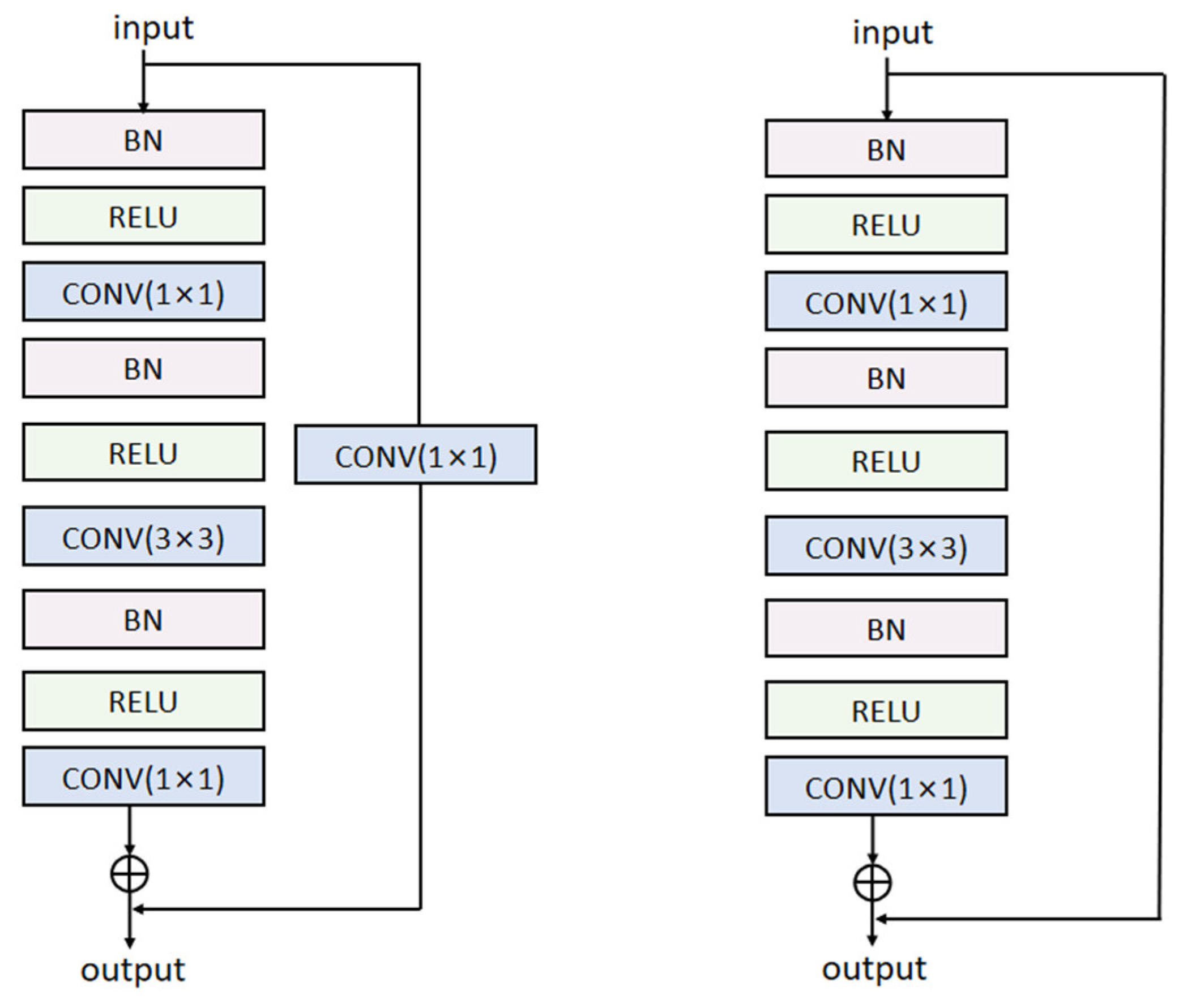
In this work, a 41-layer structure of ResNet was used to classify the cell cycle stage. Our structure was based on the model created by He et al. [22] and the residual module proposed by He et al. [34]. Figure 2 shows the model’s structure. In the residual module, the first CONV had filters of 1 × 1, the second CONV had filters of 3 × 3, and the third CONV had filters of 1 × 1.
Our ResNets were fabricated by stacking residual modules on top of one another. The numbers of residual modules were 3, 3, and 4. First, there were three residual modules, and the three CONV layers learned 32, 32, and 128 filters. Second, there were three residual modules, and the three CONV layers learned 64, 64, and 256 filters. Finally, there were four residual modules and the three CONV layers learned 128, 128, and 512 filters. The dimensions were reduced when the residual modules were stacked every time. Moreover, one CONV layer was added to the model before the residual modules, and one FC layer was added at the end of the model. As a result, the structure of our ResNet had a depth of 41 layers. The depth of our model could be changed by the number of residual modules. The structure of our model is shown in Figure 3.

3. Experiment

The whole experiment included two parts, namely, dataset generation and model training.

3.1. Dataset

A total of 32,266 original images of Jurkat cells were collected by imaging flow cytometry [14] (Jurkat dataset). The dataset was divided into seven different stages, including phases of interphase (G1, G2, and S) and phases of mitosis (prophase, anaphase, metaphase, and telophase). Figure 4 shows the original images of different cell cycle stages.
The study [14] showed the G1, G2, and S phases as the same stage. Then phases of interphase (G1/G2/S) and phases of mitosis (prophase, anaphase, metaphase, and telophase) were classified, and the accuracy of the five stages of classification was 98.73% ± 0.16%. However, when the phases of interphase (G1/G2/S) stages were separated and regarded as one stage (G1, G2, S), then seven stages of the image were classified, leading to an accuracy of 79.40% ± 0.77%. Although the G1, G2, and S phases were combined into one stage and higher classification accuracy of five stages was obtained, the accurate classification of cell cycle stages was not achieved. For the classification of a cell cycle, it was necessary not only to separate stages with excessively different morphological details, such as phases of mitosis (prophase, anaphase, metaphase, and telophase), from the other stages, but also to separate phases of interphase (G1, G2, and S) with similar morphological details.
In addition, it was clear from the original images that the number of images in the anaphase, metaphase, prophase, and telophase stages was too low, and the amount of data in different periods varied greatly, leading to inaccurate classification results. Therefore, based on the distribution of the original images of each stage, WGAN-GPs were used to increase the amounts of anaphase, metaphase, prophase, and telophase tenfold by us. In order to achieve a relative balance for the number of images in each cell cycle stage, random under-sampling was used for the G1 phase; 8610 images of the G1 stage were used for classification. The number of generated images and the number of images used for classification are shown in Table 1.
After the seven stages of cell cycle images were classified, these images were divided into four stages—phases of interphase (G1, G2, S) and phases of mitosis (M). The images of anaphase, metaphase, prophase, and telophase stages were combined into one stage, namely M, and the dataset obtained is shown in Table 2. It can be seen from Table 2 that the number of images of each stage reached a balance.

3.2. Model Training

The WGAN-GP was used to train the four stages of anaphase, metaphase, prophase, and telophase, and the batch sizes were set to 4, 16, 16, and 4, respectively, according to the number of original images. In all, 5000 epochs were set for each training process. Subsequently, the WGAN-GP model was used to generate 150, 680, 6060, and 270 images for the four stages of the cell cycle, meaning that the images for each stage were increased tenfold. For the four-stage classification of the cell cycle, the WGAN-GP model was used to generate 7,160 images of the M stage. During the process of training for WGAN-GP, the batch size was 16, and the training epoch was 5000.
The parameters of the network for classification were randomly initialized. The original size of the images was 66 × 66 × 1. All of the images were resized to 64 × 64 × 1 and divided into mini-batches for training. During the process of training for classification, the batch size was 32, the initial learning rate was 0.01, and the momentum was 0.9. The optimization strategy was the stochastic gradient descent method, and the default activation function was ReLU in the entire network.
During the classification, 60% of the images were used as the training set, 20% of the images were used as validation, and the rest of the images were used as the testing set. For the four-stages classification, the number of original images used for classification was 33,427. Moreover, 20,657 images were used for training, 6885 images were used for validation, and 6885 images were used for testing.
The environment for the experiments was Python 3.6, and the operating system was Linux with an Intel (R) Xeon (R) CPU E5-2682 v4 @ 2.50GHz processor, 32GB memory, and a Tesla P100-PCIE-16GB graphics card. The experiments were based on the open-source deep learning framework TensorFlow-gpu 2.0.0a0 and Keras 2.3.1.

4. Results

4.1. Results of Generated Images by WGAN-GP

According to the four stages of cell cycle images-anaphase, metaphase, prophase, and telophase-generated by WGAN-GP, the generated images could be used for subsequent cell cycle classification, as they were almost the same as the original cell cycle images. As such, Figure 5 shows the images generated by WGAN-GP.
In order to verify the effectiveness of WGAN-GP, the following sets of classification experiments were conducted. The compared results are shown in Table 3 and Table 4. The results for the original images, the images generated by WGAN-GP, the original images after under-sampling, and the images generated by WGAN-GP after under-sampling were compared with each other.
As shown in Table 3 and Table 4, the seven-stage classification accuracy of the original images and the four-stage classification accuracy of the original images were 78.37% and 78.35%, respectively. The seven-stage classification accuracy of images generated by WGAN-GP and the four-stage classification accuracy of images generated by WGAN-GP were 82.25% and 82.10%, respectively. The seven-stage classification accuracy and the four-stage classification accuracy improved by 3.88% and 3.75%, respectively.
In order to obtain balanced images, random under-sampling was used for the stage of G1. The seven-stage classification accuracy of original images after under-sampling and the four-stage classification accuracy of original images after under-sampling were 78.32% and 77.16%, respectively. The seven-stage classification accuracy of images generated by WGAN-GP after under-sampling and the four-stage classification accuracy of images generated by WGAN-GP after under-sampling were 83.60% and 83.88%, respectively. The seven-stage classification accuracy and the four-stage classification accuracy were improved by 5.28% and 6.72%, respectively. From these results, it was clear that the seven-stage classification accuracy and the four-stage classification accuracy were improved by WGAN-GP.
Moreover, the four-stage classification accuracy was reduced by about 1.15% when the images of the M stage were original, and the images of the G1 stage were under-sampled. Additionally, when WGAN-GP was used to augment the images of the M stage, the G1 stage was under-sampled. In other words, the number of images for each stage was basically balanced, and the four-stage classification accuracy was almost unaffected. When compared, the result showed that the classification accuracy could be effectively improved by using WGAN-GP for data augmentation.

4.2. Results of Classification

For imbalanced image classification, it was difficult to accurately reflect the performance of the classifier by using accuracy alone. It was necessary to combine other evaluation indicators, such as F-Score, G-means metric, and the receiver operating characteristic (ROC) curve [35,36]. The F-Score is directly related to recall and precision. This method was mainly to maximize recall and precision as much as possible so the classification performance for majority categories and minority categories could be correctly evaluated.
Accuracy = (TP + TN)/(TP + TN + FP + FN)
F - Score = Recall   ×   Precision = TP / ( TP + FN ) × TP / ( TP + FP )
The ROC curve was drawn with the classification error rate of the majority class as the abscissa and the classification accuracy rate of the minority class as the ordinate. The ROC curve is currently one of the commonly used methods to evaluate the performance of classifiers on imbalanced data sets.
Table 5 shows the seven-stage classification result for the original images. Additionally, Table 6 shows the seven-stage classification result after using WGAN-GP. In Table 5, the precision of anaphase, metaphase, and telophase was almost 0. One of the reasons was that the number of original images for these stages was too low, and the number of images in the test set was too low. Another reason might be the acquisition of original images. The process by which we obtained the original images was dynamic and changed over time. When the images of a certain stage were acquired, the cells might be dynamically changing, which would not only cause images to have the characteristics of this stage, but they might also contain the characteristics of other stages. This made the original images difficult to classify correctly. The obtained results had large deviations, and the weighted average accuracy of the classification was 78.35%. The accuracy of each stage was 0, 83.16%, 84.56%, 0, 85.21%, 67.65%, and 0. In Table 6, the images generated by WGAN-GP of anaphase, metaphase, prophase, and telophase were used for classification, and the weighted average accuracy of the classification was 82.10%. Compared with the accuracy of original images, the average accuracy increased by 3.75%. Additionally, the accuracy of each stage was 100%, 81.81%, 84.56%, 81.25%, 99.34%, 67.00%, and 100%. It could be seen from Table 5 and Table 6 that the classification accuracies of the anaphase, the metaphase, the prophase, and the telophase stages were significantly improved by WGAN-GP.
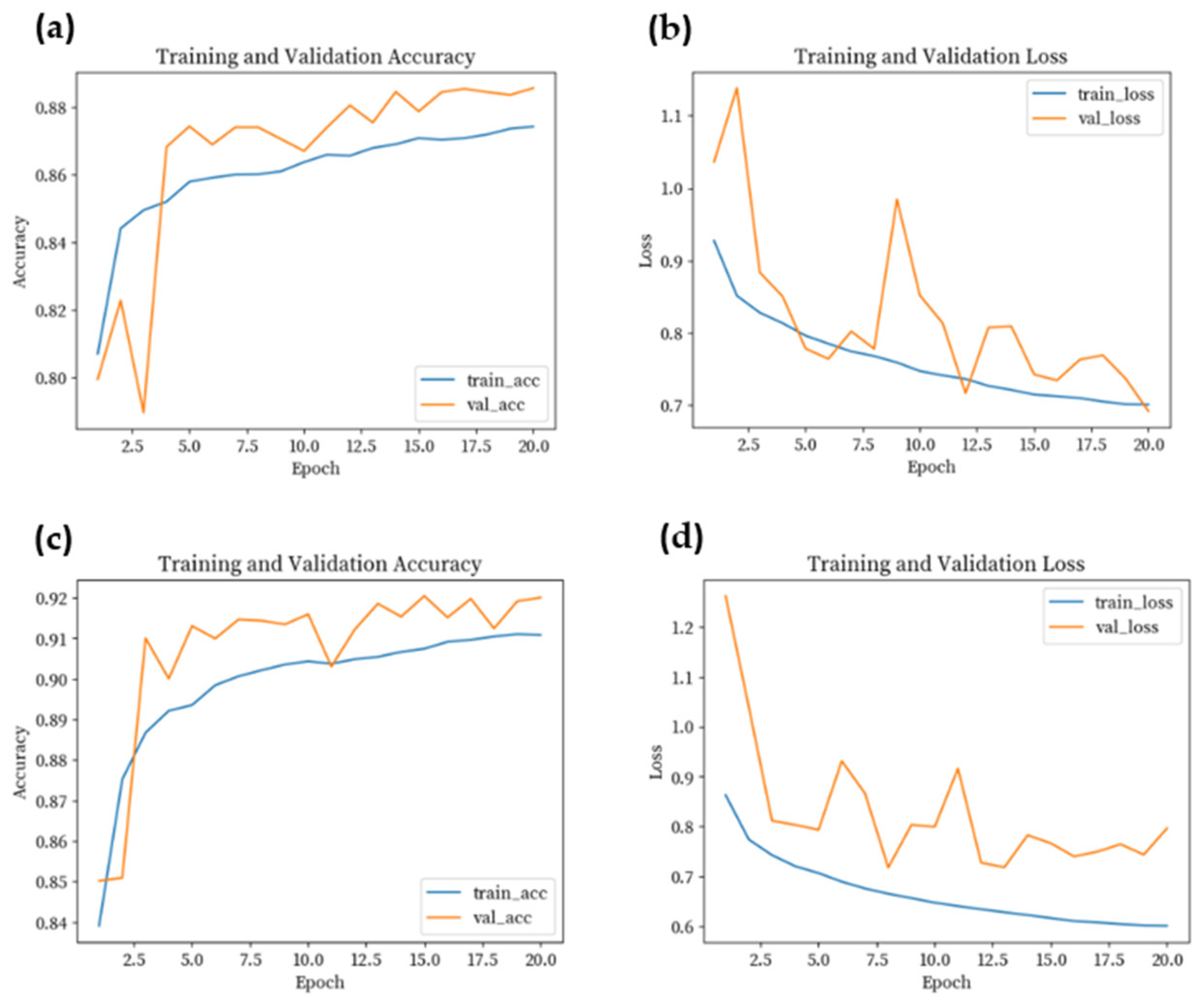
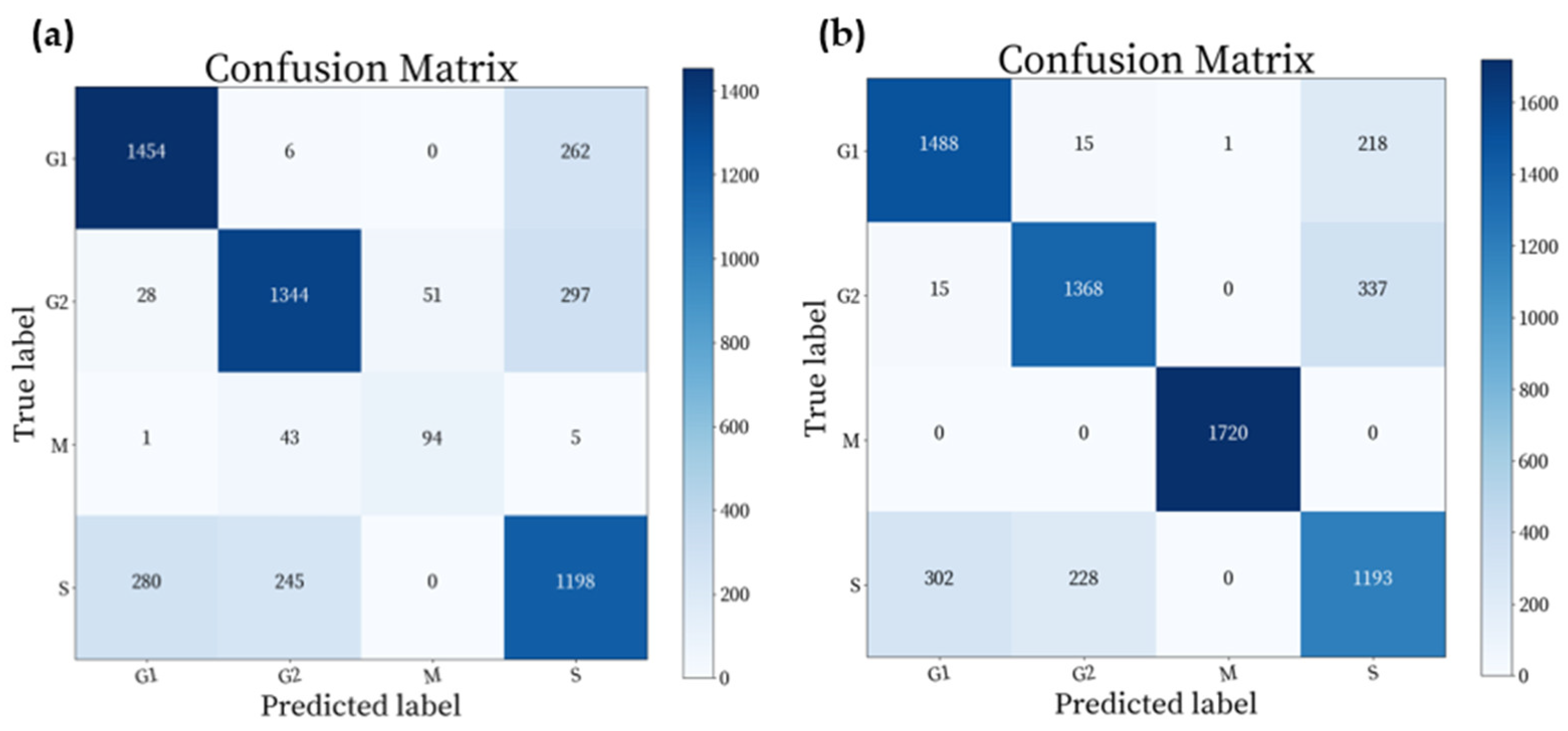
In addition, the combined dataset (G1, G2, M, and S phase) was used for classification. The classification results for the original images of the M stage and the classification results for the generated images of the M stage are shown in Table 7 and Table 8, respectively. In Table 7, the weighted average accuracy of the classification was 77.16%, and the accuracy of each stage was 82.47%, 82.05%, 64.83%, and 67.99%. In Table 8, the generated images of the M stage were used for classification, and the weighted average accuracy of the classification was 83.88%. Compared with the accuracy of the original images, the weighted average accuracy has increased by 6.72%. Additionally, the accuracy of each stage was 82.44%, 84.92%, 99.94%, and 68.25%. It can be seen from Table 7 and Table 8 that the classification accuracy of the M stage was significantly improved by WGAN-GP. Figure 6 shows the training and validation accuracy with training epochs. Figure 7 is the result represented by a confusion matrix. Figure 8 shows the ROC curve for four-stage classification.

4.3. Verification of Results with New Dataset

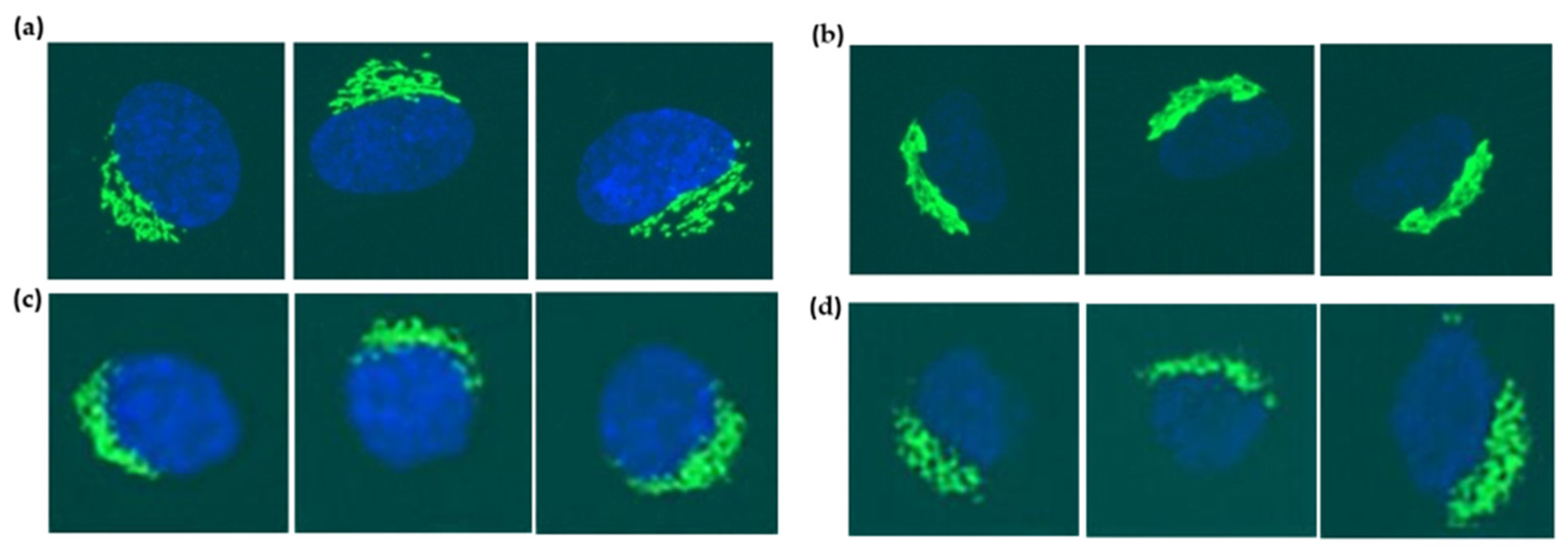
In order to verify the effectiveness of our model, another cell cycle data set was used. Nagao et al. [13] collected fluorescence microscope images of different cell cycles containing subcellular structures, such as the nucleus, the Golgi apparatus, and the microtubule cytoskeleton (HeLa dataset). The classification of different cycle stages could be carried out by extracting the characteristics of these subcellular structures. The data set contained only two categories, namely G2 and non-G2. The cell cycle images of the G2 phase were regarded as one class, and the images of the G1 phase and the S phase were regarded as one class. The images of the M phase were not in this data set. The numbers of images in the G2 class and the non-G2 class were each 922. The original images of the G2 class and the non-G2 class are shown in Figure 9. The WGAN-GP was used to generate images for the G2 class and the non-G2 class, and the generated images are shown in Figure 9.
Although the original images of this data set were balanced, data augmentation was carried out on this data set to verify the effects of WGAN-GP. Each class used WGAN-GP to generate 10,000 images and used random under-sampling to obtain 9220 images. Then, the 9220 images were used for classification. The results of the classification for the original images and generated images are shown in Table 9.
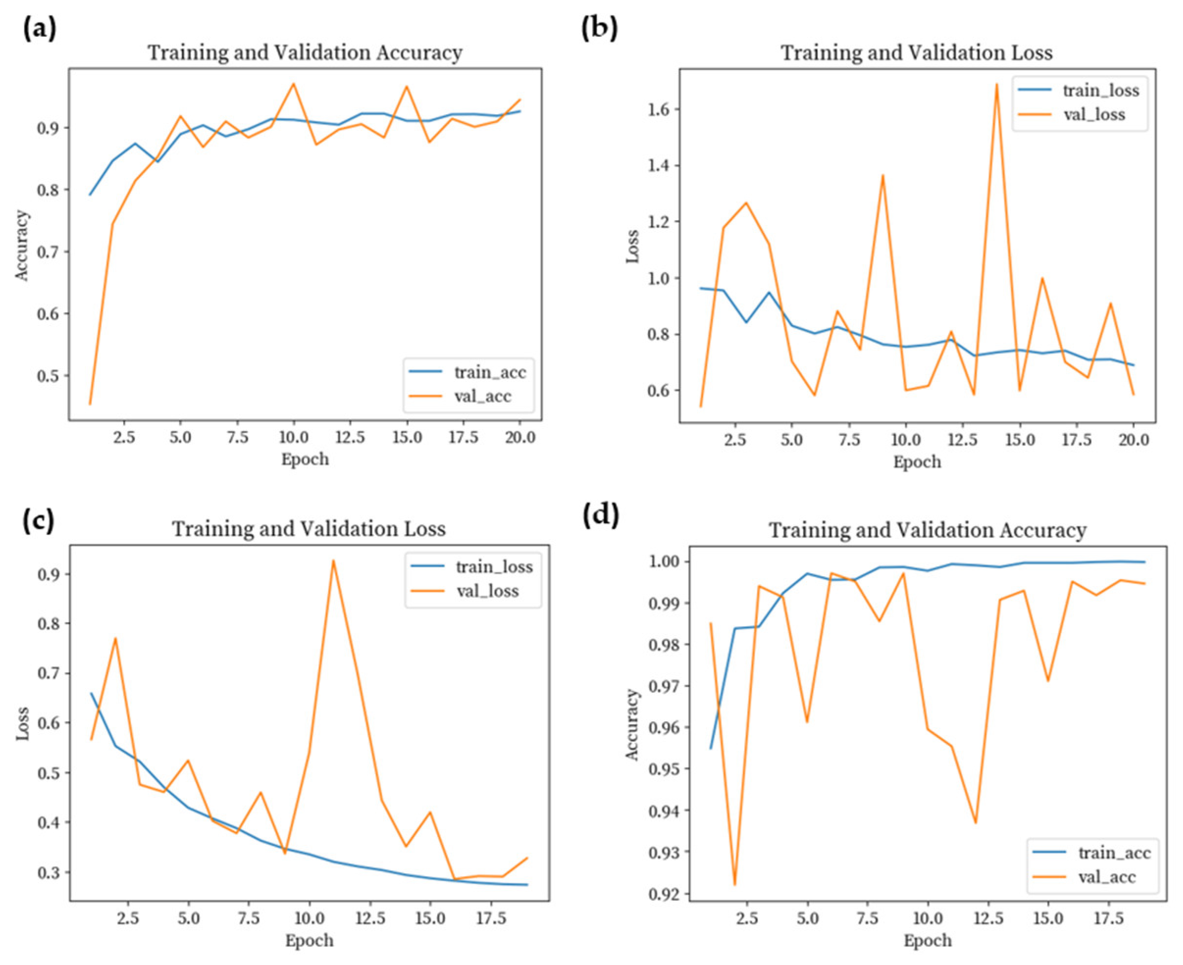
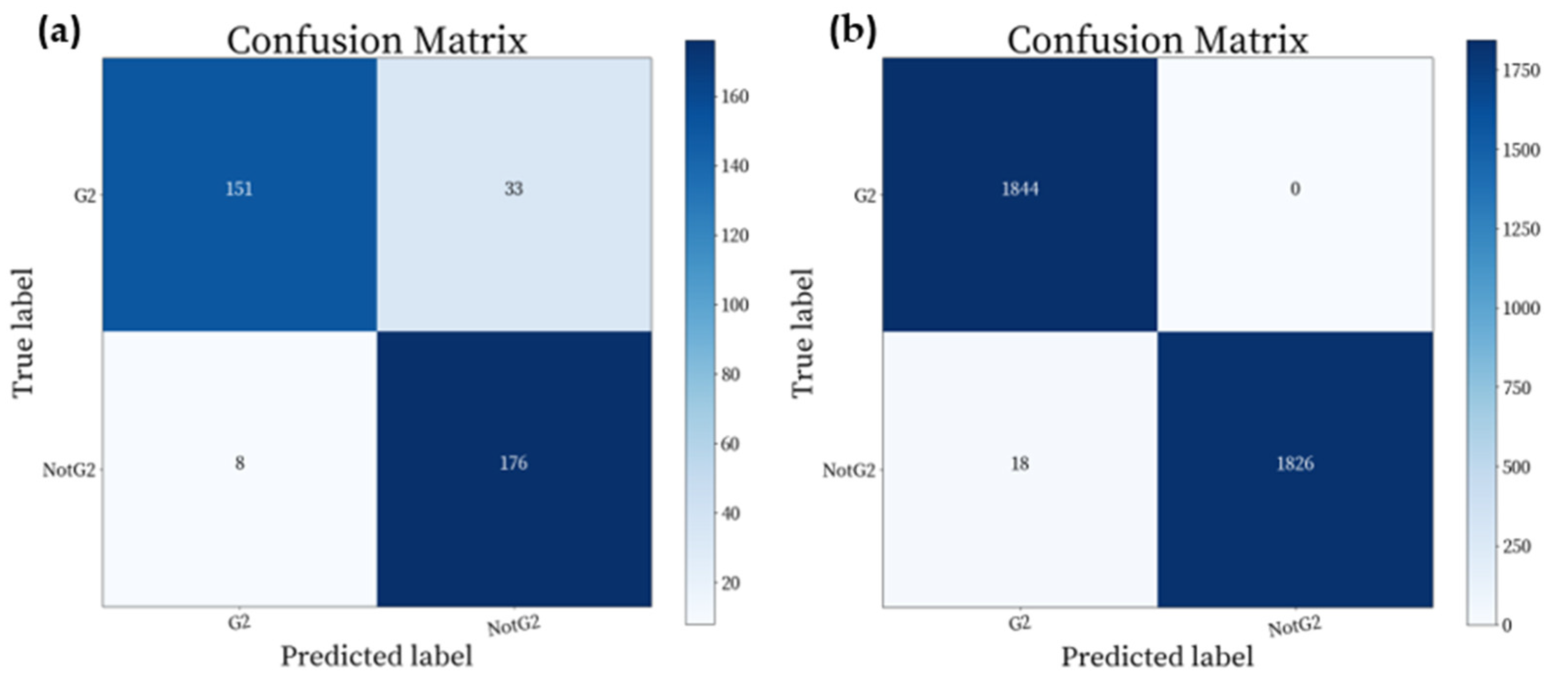
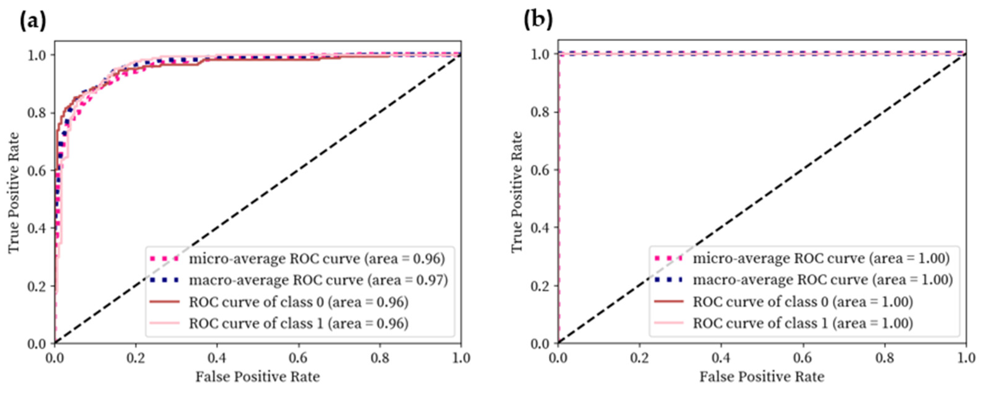
As shown in Table 9, the average accuracy of classification for original images was 87.63%, and the average accuracy of classification for generated images was 97.65%. Compared with the accuracy of original images, the average accuracy increased by 10.02%. The classification accuracy was significantly improved by WGAN-GP. Figure 10 shows the training and validation accuracy with training epochs. Figure 11 is the result as represented by a confusion matrix. Figure 12 shows the ROC curve for classification.

5. Discussion

To verify the effect of our method, the classification results for the same data set were compared with those of the existing methods in the literature, and the results are shown in Table 10, Table 11 and Table 12. In Table 10, the classification accuracy of anaphase, metaphase, prophase, and telophase improved by 80%, 69.49%, 38.62%, and 3.71%, respectively. In Table 11, the classification accuracy of the M phase improved by 55.9%. In Table 12, the classification accuracy improved by 12.52%. In fact, the classification accuracy was significantly improved by WGAN-GP. Therefore, WGAN-GP can be used to improve the classification of imbalanced cell cycle phases.
According to the original images of the Jurkat dataset, it was apparent from their characteristics that, except for the phase of mitosis (M), the cell cycle images of the other stages were difficult to distinguish, even for experts in the field of cell cycles. If the grayscale images of different stages were placed in the order of a cell cycle phase and the experts were informed, the stages might be classified by some morphological features. However, if the grayscale images of different stages were randomly placed, it was difficult for experts to classify the different stages. This was precise because the differences between images of different cell cycle stages were not obvious. It was also difficult to use ResNet to further enhance classification accuracy.
In general, determining the cell cycle phase requires the fluorescent labeling of cells, and fluorescent staining is a very complicated process. In this study, we used a deep learning framework to classify the brightfield images without fluorescent staining to easily recognize the cells in the different stages; this was a process that was important for reducing the difficulty of operations in cell cycle classification. Furthermore, different phases of the cell cycle lasted for different durations, which inevitably led to an imbalance in the number of acquired images at different stages. Therefore, the use of a WGAN-GP could solve problems related to imbalanced cell cycle images. Additionally, from the perspective of practical applications in the field, the use of a WGAN-GP was of great significance for the classification of the cell cycle.
These problems also reflected the difficulty in obtaining biomedical images. In some cases, time and money were required to obtain sufficient images; without high-quality images, it might be difficult to perform subsequent experiments. Follow-up experiments would certainly benefit if they were to use our method for data augmentation.

6. Conclusions

In this paper, deep learning technology was applied to the field of cell cycle classification, and a cell cycle classification framework based on the combination of WGAN-GP and ResNet was used. This combination yielded better classification results than the original classification framework. The WGAN-GP was used for data augmentation, and the ResNet was used for classification. The Jurkat dataset was used for the seven-stage and four-stage classification of the cell cycle, and better classification results were obtained than those found in previous papers. Additionally, another dataset (HeLa dataset) was used to validate the results of our model. By introducing the WGAN-GP network to generate additional cell cycle images, the problem of insufficient original images was solved. The imbalance between different cell cycle stages was reduced, and classification accuracy was improved.
In the future, we will continue to improve the structure of the network for classification, and we will try to use a network other than WGAN-GP for data augmentation. We will use other methods to obtain cell cycle images without a fluorescent label, and we will classify them in this framework to further improve the classification accuracy of the cell cycle, finally achieving the label-free classification of cell cycle images.

Author Contributions

Project administration, Y.Z.; software, X.J.; supervision, Y.Z.; writing—original draft, X.J.; writing—review & editing, Y.Z. and Z.H. All authors have read and agreed to the published version of the manuscript.

Funding

This research did not receive any specific grant from funding agencies in the public, commercial, or not-for-profit sectors.

Institutional Review Board Statement

Not applicable.

Informed Consent Statement

Not applicable.

Data Availability Statement

The data presented in this study are openly available at doi:10.1038/s41467-017-00623-3, reference number [14]. This data can be found here: https://github.com/theislab/deepflow (accessed on 11 June 2021).

Conflicts of Interest

The authors declare no conflict of interest.

References

  1. Fang, H.-S.; Lang, M.-F.; Sun, J. New Methods for Cell Cycle Analysis. Chin. J. Anal. Chem. 2019, 47, 1293–1301. [Google Scholar] [CrossRef]
  2. Roukos, V.; Pegoraro, G.; Voss, T.C.; Misteli, T. Cell cycle staging of individual cells by fluorescence microscopy. Nat. Protoc. 2015, 10, 334–348. [Google Scholar] [CrossRef] [PubMed]
  3. Matuszewski, D.J.; Sintorn, I.-M.; Puigvert, J.C.; Wählby, C. Comparison of Flow Cytometry and Image-Based Screening for Cell Cycle Analysis. Nat. Comput. Ser. 2016, 623–630. [Google Scholar] [CrossRef] [Green Version]
  4. Schönenberger, F.; Deutzmann, A.; Ferrando-May, E.; Merhof, D. Discrimination of cell cycle phases in PCNA-immunolabeled cells. BMC Bioinform. 2015, 16, 3262. [Google Scholar] [CrossRef] [PubMed] [Green Version]
  5. Sakaue-Sawano, A.; Kurokawa, H.; Morimura, T.; Hanyu, A.; Hama, H.; Osawa, H.; Kashiwagi, S.; Fukami, K.; Miyata, T.; Miyoshi, H.; et al. Visualizing Spatiotemporal Dynamics of Multicellular Cell-Cycle Progression. Cell 2008, 132, 487–498. [Google Scholar] [CrossRef] [Green Version]
  6. Bajar, B.T.; Lam, A.J.; Badiee, R.; Oh, Y.-H.; Chu, J.; Zhou, X.X.; Kim, N.; Kim, B.B.; Chung, M.; Yablonovitch, A.L.; et al. Fluorescent indicators for simultaneous reporting of all four cell cycle phases. Nat. Methods 2016, 13, 993–996. [Google Scholar] [CrossRef] [Green Version]
  7. Ferro, A.; Mestre, T.; Carneiro, P.; Sahumbaiev, I.; Seruca, R.; Sanches, J.M. Blue intensity matters for cell cycle profiling in fluorescence DAPI-stained images. Lab. Investig. 2017, 97, 615–625. [Google Scholar] [CrossRef] [Green Version]
  8. Blasi, T.; Hennig, H.; Summers, H.D.; Theis, F.J.; Cerveira, J.; Patterson, J.O.; Davies, D.; Filby, A.; Carpenter, A.E.; Rees, P. Label-free cell cycle analysis for high-throughput imaging flow cytometry. Nat. Commun. 2016, 7, 10256–10264. [Google Scholar] [CrossRef] [Green Version]
  9. Khan, S.; Islam, N.; Jan, Z.; Din, I.U.; Rodrigues, J.J.P.C. A novel deep learning based framework for the detection and classification of breast cancer using transfer learning. Pattern Recognit. Lett. 2019, 125, 1–6. [Google Scholar] [CrossRef]
  10. Araújo, F.H.; Silva, R.R.; Ushizima, D.M.; Rezende, M.T.; Carneiro, C.M.; Bianchi, A.G.C.; Medeiros, F.N. Deep learning for cell image segmentation and ranking. Comput. Med. Imaging Graph. 2019, 72, 13–21. [Google Scholar] [CrossRef]
  11. Kurnianingsih; Allehaibi, K.H.S.; Nugroho, L.E.; Widyawan; Lazuardi, L.; Prabuwono, A.S.; Mantoro, T. Segmentation and Classification of Cervical Cells Using Deep Learning. IEEE Access 2019, 7, 116925–116941. [Google Scholar] [CrossRef]
  12. Dürr, O.; Sick, B. Single-Cell Phenotype Classification Using Deep Convolutional Neural Networks. J. Biomol. Screen. 2016, 21, 998–1003. [Google Scholar] [CrossRef] [PubMed] [Green Version]
  13. Nagao, Y.; Sakamoto, M.; Chinen, T.; Okada, Y.; Takao, D. Robust classification of cell cycle phase and biological feature extraction by image-based deep learning. Mol. Biol. Cell 2020, 31, 1346–1354. [Google Scholar] [CrossRef] [PubMed]
  14. Eulenberg, P.; Köhler, N.; Blasi, T.; Filby, A.; Carpenter, A.E.; Rees, P.; Theis, F.J.; Wolf, F.A. Reconstructing cell cycle and disease progression using deep learning. Nat. Commun. 2017, 8, 1–6. [Google Scholar] [CrossRef] [Green Version]
  15. Susan, S.; Kumar, A. SSO Maj -SMOTE- SSO Min: Three-step intelligent pruning of majority and minority samples for learning from imbalanced datasets. Appl. Soft Comput. 2019, 78, 141–149. [Google Scholar] [CrossRef]
  16. Susan, S.; Kumar, A. Learning Data Space Transformation Matrix from Pruned Imbalanced Datasets for Nearest Neighbor Classification. In Proceedings of the 2019 IEEE 21st International Conference on High Performance Computing and Communications; IEEE 17th International Conference on Smart City; IEEE 5th International Conference on Data Science and Systems (HPCC/SmartCity/DSS), Zhangjiajie, China, 10–12 August 2019; pp. 2831–2838. [Google Scholar]
  17. Frid-Adar, M.; Diamant, I.; Klang, E.; Amitai, M.; Goldberger, J.; Greenspan, H. GAN-based synthetic medical image augmentation for increased CNN performance in liver lesion classification. Neurocomputing 2018, 321, 321–331. [Google Scholar] [CrossRef] [Green Version]
  18. Saini, M.; Susan, S. Deep transfer with minority data augmentation for imbalanced breast cancer dataset. Appl. Soft Comput. 2020, 97, 106759. [Google Scholar] [CrossRef]
  19. Rubin, M.; Stein, O.; Turko, N.A.; Nygate, Y.; Roitshtain, D.; Karako, L.; Barnea, I.; Giryes, R.; Shaked, N.T. TOP-GAN: Stain-free cancer cell classification using deep learning with a small training set. Med. Image Anal. 2019, 57, 176–185. [Google Scholar] [CrossRef] [PubMed] [Green Version]
  20. Zheng, M.; Li, T.; Zhu, R.; Tang, Y.; Tang, M.; Lin, L.; Ma, Z. Conditional Wasserstein generative adversarial network-gradient penalty-based approach to alleviating imbalanced data classification. Inf. Sci. 2020, 512, 1009–1023. [Google Scholar] [CrossRef]
  21. Arjovsky, M.; Chintala, S.; Bottou, L. Wasserstein generative adversarial networks. In Proceedings of the Thirty-fourth International Conference on Machine Learning (ICML), Sydney, Australia, 6–11 August 2017; pp. 214–223. [Google Scholar]
  22. He, K.; Zhang, X.; Ren, S.; Sun, J. Deep residual learning for image recognition. In Proceedings of the IEEE Conference on Computer Vision and Pattern Recognition, Las Vegas, NV, USA, 27–30 June 2016; pp. 770–778. [Google Scholar]
  23. Goodfellow, I.; Pouget-Abadie, J.; Mirza, M.; Xu, B.; Warde-Farley, D.; Ozair, S.; Courville, A.; Bengio, Y. Generative adversarial nets. Adv. Neural Inf. Process. Syst. 2014, 27, 2672–2680. [Google Scholar]
  24. Gulrajani, I.; Ahmed, F.; Arjovsky, M.; Dumoulin, V.; Courville, A. Generative Adversarial Nets. Adv. Neural Inf. Process. Syst. 2017, 31, 5767–5777. [Google Scholar]
  25. Ma, L.; Shuai, R.; Ran, X.; Liu, W.; Ye, C. Combining DC-GAN with ResNet for blood cell image classification. Med. Biol. Eng. Comput. 2020, 58, 1251–1264. [Google Scholar] [CrossRef] [PubMed]
  26. Dimitrakopoulos, P.; Sfikas, G.; Nikou, C. ISING-GAN: Annotated Data Augmentation with a Spatially Constrained Generative Adversarial Network. In Proceedings of the 2020 IEEE 17th International Symposium on Biomedical Imaging (ISBI), Iowa City, IA, USA, 3–7 April 2020; pp. 1600–1603. [Google Scholar]
  27. Chen, S.; Shi, D.; Sadiq, M.; Cheng, X. Image Denoising With Generative Adversarial Networks and its Application to Cell Image Enhancement. IEEE Access 2020, 8, 82819–82831. [Google Scholar] [CrossRef]
  28. Lin, H.; Hu, Y.; Chen, S.; Yao, J.; Zhang, L. Fine-Grained Classification of Cervical Cells Using Morphological and Appearance Based Convolutional Neural Networks. IEEE Access 2019, 7, 71541–71549. [Google Scholar] [CrossRef]
  29. Lei, H.; Han, T.; Zhou, F.; Yu, Z.; Qin, J.; Elazab, A.; Lei, B. A deeply supervised residual network for HEp-2 cell classification via cross-modal transfer learning. Pattern Recognit. 2018, 79, 290–302. [Google Scholar] [CrossRef]
  30. Baykal, E.; Dogan, H.; Ercin, M.E.; Ersoz, S.; Ekinci, M. Modern convolutional object detectors for nuclei detection on pleural effusion cytology images. Multimed. Tools Appl. 2019, 1–20. [Google Scholar] [CrossRef]
  31. Evangeline, I.K.; Precious, J.G.; Pazhanivel, N.; Kirubha, S.P.A. Automatic Detection and Counting of Lymphocytes from Immunohistochemistry Cancer Images Using Deep Learning. J. Med. Biol. Eng. 2020, 40, 735–747. [Google Scholar] [CrossRef]
  32. Gouda, N.; Amudha, J. Skin Cancer Classification using ResNet. In Proceedings of the 2020 IEEE 5th International Conference on Computing Communication and Automation (ICCCA), Greater Noida, India, 30–31 October 2020; pp. 536–541. [Google Scholar]
  33. Shemona, J.S.; Kumar, A. Novel segmentation techniques for early cancer detection in red blood cells with deep learning based classifier-a comparative approach. IET Image Process. 2020, 14, 1726–1732. [Google Scholar] [CrossRef]
  34. He, K.; Zhang, X.; Ren, S.; Sun, J. Identity Mappings in Deep Residual Networks. In European Conference on Computer Vision; Springer Science and Business Media LLC: Cham, Switzerland, 2016; pp. 630–645. [Google Scholar]
  35. Ramos-López, D.; Maldonado, A.D. Cost-Sensitive Variable Selection for Multi-Class Imbalanced Datasets Using Bayesian Networks. Mathematics 2021, 9, 156. [Google Scholar] [CrossRef]
  36. Zhang, C.; Tan, K.C.; Li, H.; Hong, G.S. A Cost-Sensitive Deep Belief Network for Imbalanced Classification. IEEE Trans. Neural Netw. Learn. Syst. 2018, 30, 109–122. [Google Scholar] [CrossRef] [PubMed] [Green Version]
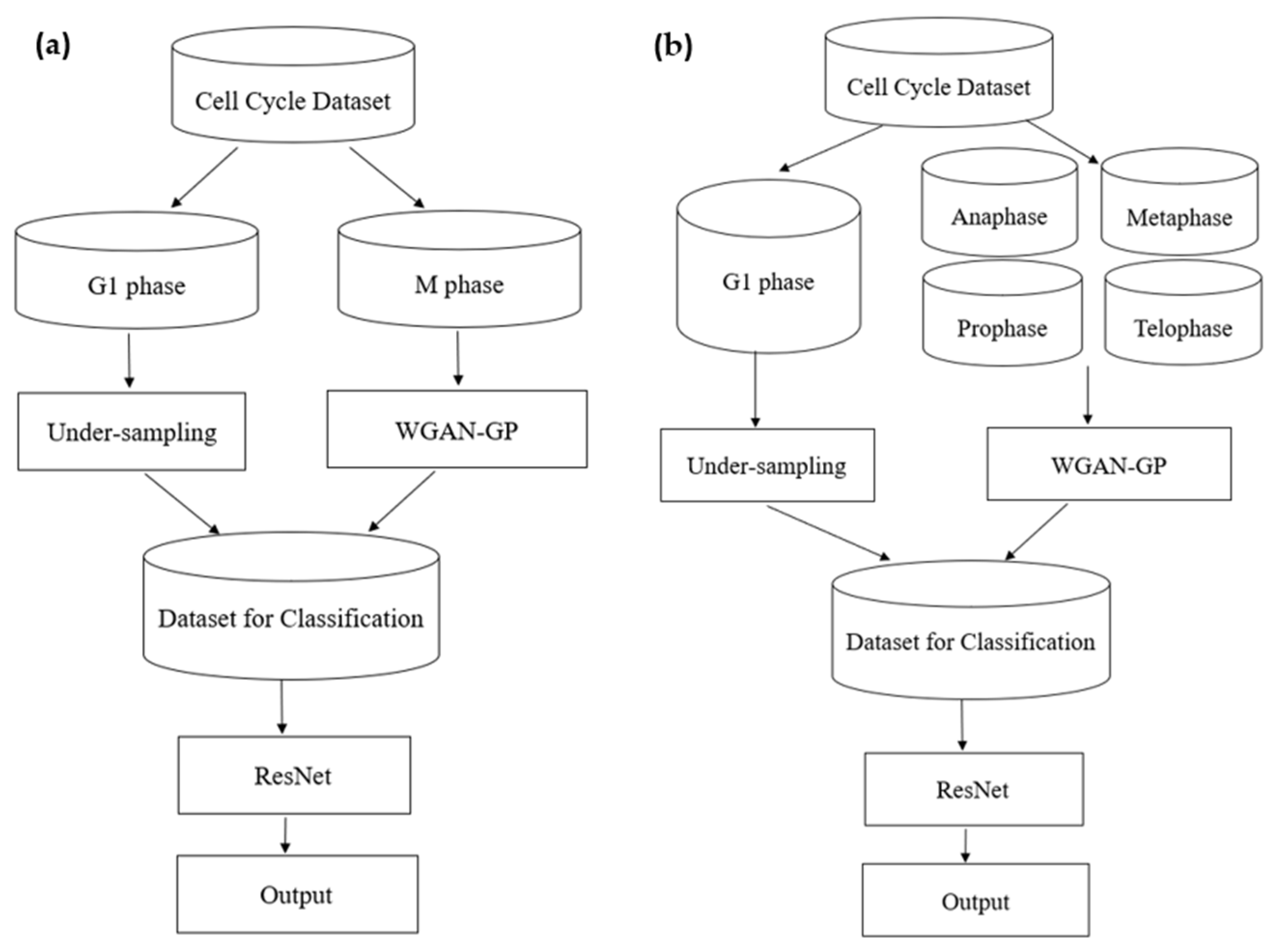
Figure 1. Overview of the framework for our model. (a) The framework of four stages of classification; (b) the framework of seven stages of classification.
Information 12 00249 g001
Figure 2. The structure of the residual module.
Information 12 00249 g002
Figure 3. The structure of our ResNet model.
Information 12 00249 g003
Figure 4. The original images of different cell cycle stages.
Information 12 00249 g004
Figure 5. The generated images of different cell cycle stages.
Information 12 00249 g005
Figure 6. The training and validation accuracy and loss versus the number of training epochs. (a) Accuracy of four stages classification for original images; (b) loss of four stages classification for original images; (c) accuracy of four stages classification for generated images; (d) loss of four stages classification for generated images.
Information 12 00249 g006
Figure 7. The confusion matrix of classification. (a) Four-stage classification of original images; (b) four-stages classification of generated images.
Information 12 00249 g007
Figure 8. The ROC curves of classification. (a) Four-stage classification of original images; (b) four-stage classification of generated images.
Information 12 00249 g008
Figure 9. The images of the G2 class and the non-G2 class. (a) Images of G2 class [13]; (b) images of non-G2 class [13]; (c) images generated by WGAN-GP of G2 class; (d) images generated by WGAN-GP of non-G2 class.
Information 12 00249 g009
Figure 10. The training and validation accuracy and loss versus the number of training epochs. (a) Accuracy of two-class classification for original images; (b) loss of two-class classification for original images; (c) accuracy of two-class classification for generated images; (d) loss of two-class classification for generated images.
Information 12 00249 g010
Figure 11. The confusion matrix of classification. (a) Two-class classification of original images; (b) two-class classification of generated images.
Information 12 00249 g011
Figure 12. The ROC curves for classification. (a) Two-class classification of original images; (b) two-class classification of generated images.
Information 12 00249 g012
Table 1. The number of images of different cell cycle stages and the number of images used for seven stages.
Cell Cycle StagesThe Number of Original ImagesThe Number of Generated Images by WGAN-GPThe Number of Images Used for Classification
Classification 1Classification 2Classification 3Classification 4
Anaphase151501515150150
G114,333-14,333861014,3338610
G28601-8601860186018601
Metaphase686806868680680
Prophase606606060660660606060
S8616-8616861686168616
Telophase272702727270270
Table 2. The number of images of different cell cycle stages and the number of images used for four stages.
Cell Cycle StagesThe Number of Original ImagesThe Number of Generated Images by WGAN-GPThe Number of Images Used for Classification
Classification 1Classification 2Classification 3Classification 4
G114,333-14,333861014,3338610
G28601-8601860186018601
M716716071671671607160
S8616-8616861686168616
Table 3. Seven-stage classification results of the original images, the images generated by WGAN-GP, the original images after under-sampling, and the images generated by WGAN-GP after under-sampling.
Cell Cycle StagesThe Number of Original ImagesThe Number of Images Generated by WGAN-GPThe Number of Original Images after Under-Sampling The Number of Images Generated by WGAN-GP after Under-Sampling
Anaphase1515015150
G114,33314,33386108610
G28601860186018601
Metaphase6868068680
Prophase60660606066060
S8616861686168616
Telophase2727027270
Weighted_Avg0.78370.82250.78350.8210
Table 4. Four-stage classification results for the original images, the images generated by WGAN-GP, the original images after under-sampling, and the images generated by WGAN-GP after under-sampling.
Cell Cycle StagesThe Number of Original ImagesThe Number of Images Generated by WGAN-GPThe Number of Original Images after Under-SamplingThe Number of Images Generated by WGAN-GP after Under-Sampling
G114,33314,33386108610
G28601860186018601
M71671607167160
S8616861686168616
Weighted_Avg0.78320.83600.77160.8388
Table 5. The seven-stage classification results for the original images.
Cell Cycle StagesPrecisionRecallF1-ScoreSupport
Anaphase0.00000.00000.00003
G10.83160.84030.83591722
G20.84530.80120.82411720
Metaphase0.00000.00000.000013
Prophase0.85211.00000.9202121
S0.67650.70520.69051723
Telophase0.00000.00000.00005
Weight_Avg0.78350.78440.78355307
Table 6. The seven-stage classification results for images generated by WGAN-GP.
Cell Cycle StagesPrecisionRecallF1-ScoreSupport
Anaphase1.00000.06670.125030
G10.81810.84900.83331722
G20.84560.78950.81661720
Metaphase0.81250.95590.8784136
Prophase0.99340.99090.99221212
S0.67000.69180.68081723
Telophase1.00001.00001.000054
Weight_Avg0.82100.81840.81746597
Table 7. The four-stage classification results for original images.
Cell Cycle StagesPrecisionRecallF1-ScoreSupport
G10.82470.84440.83441722
G20.82050.78140.80051720
M0.64830.65730.6528143
S0.67990.69530.68751723
Weighted_Avg0.77160.77050.77085308
Table 8. The four-stage classification results for images generated by WGAN-GP.
Cell Cycle StagesPrecisionRecallF1-ScoreSupport
G10.82440.86410.84381722
G20.84920.79530.82141720
M0.99941.00000.99971720
S0.68250.69240.68741723
Weighted_Avg0.83880.83790.83806885
Table 9. The classification results for original images and generated images.
The Result of the Classification for Original ImagesThe Result of the Classification for Generated Images
ClassPrecisionRecallF1-ScoreSupportClassPrecisionRecallF1-ScoreSupport
G20.94970.82070.8805184G20.99031.00000.99511844
Not-G20.84210.95650.8957184Not-G21.00000.99020.99511844
Avg0.89590.88860.8881368Avg0.99520.99510.99513688
Table 10. The seven-stage classification accuracy on the same dataset (Jurkat datasets).
ModelMethodImagesAccuracy
G1G2SAnaMetaProTeloWeighted_Avg
Eulenber [14]Deep learning
(ResNet)
Dataset186.47%64.86%84.16%20%11.76%60.72%96.29%/
Model1ResNetDataset1 + WGAN-GP (Ana, Meta, Pro, Telo)81.81%84.56%67.00%100%81.25%99.34%100%82.10%
Table 11. The four-stage classification accuracy on the same dataset (Jurkat datasets).
ModelMethodImagesAccuracy
G1G2MSWeighted_Avg
Blasi [8]feature extraction
Boosting algorithm
Dataset1
Random under-sampling
70.24%96.78%44.04%90.13%/
Model2ResNet
WGAN-GP
Dataset182.47%82.05%64.83%67.99%77.16%
Model3ResNet
WGAN-GP
Dataset1 + WGAN-GP (M)82.44%84.92%99.94%68.25%83.88%
Table 12. The two-class classification accuracy on the same dataset (Hela datasets).
ModelMethodImagesAccuracy
G2NotG2Weighted_Avg
Nagao [13]CNNDataset2//87%
Model2ResNet
WGAN-GP
Dataset2 + WGAN-GP99.03%100%99.52%
Publisher’s Note: MDPI stays neutral with regard to jurisdictional claims in published maps and institutional affiliations.