A Hybrid Model for Air Quality Prediction Based on Data Decomposition

Abstract

Accurate and reliable air quality predictions are critical to the ecological environment and public health. For the traditional model fails to make full use of the high and low frequency information obtained after wavelet decomposition, which easily leads to poor prediction performance of the model. This paper proposes a hybrid prediction model based on data decomposition, choosing wavelet decomposition (WD) to generate high-frequency detail sequences WD(D) and low-frequency approximate sequences WD(A), using sliding window high-frequency detail sequences WD(D) for reconstruction processing, and long short-term memory (LSTM) neural network and autoregressive moving average (ARMA) model for WD(D) and WD(A) sequences for prediction. The final prediction results of air quality can be obtained by accumulating the predicted values of each sub-sequence, which reduces the root mean square error (RMSE) by 52%, mean absolute error (MAE) by 47%, and increases the goodness of fit (R²) by 18% compared with the single prediction model. Compared with the mixed model, reduced the RMSE by 3%, reduced the MAE by 3%, and increased the R² by 0.5%. The experimental verification found that the proposed prediction model solves the problem of lagging prediction results of single prediction model, which is a feasible air quality prediction method.

1. Introduction

Over the past few decades, air pollution had become one of the major problems afflicting most developing countries [1]. China is the largest developing country in the world and many cities have suffered from more serious air pollution problems in the past few years, such as Tianjin, Beijing, Shijiazhuang, Tangshan, Cangzhou, etc. Short-term environmental pollution can cause serious health damage, such as eye irritation, breathing difficulties, and lung and cardiovascular health effects [2].Long-term exposure to high levels of air pollutants may lead to chronic diseases such as chronic bronchitis, chronic heart failure, and chronic respiratory diseases etc. People with heart and lung disease, diabetics, the elderly and children are vulnerable to health effects related to air pollution. In addition, these pollutants and their derivatives can cause many adverse effects on the environment [3,4,5], including visibility impairment, acid deposition, global climate change, and water quality degradation. This shows that efficient and accurate air quality prediction models are important for early warning of susceptible populations and preventing diseases induced by exposure to air pollutants.

Air quality evaluation indicators include criteria air pollutants and air quality index (AQI) [6].The AQI is a comprehensive unitless quantitative description of air quality, consisting of six major pollutants: fine particulate matter (PM2.5), respirable particulate matter (PM10), carbon monoxide (CO), ozone (O₃), sulfur dioxide (SO₂), and nitrogen dioxide (NO₂). The AQI is used to measure the overall quality of the air and classifies it into six levels (good, moderate, lightly polluted, moderately polluted, heavily polluted, and severely polluted), providing a good reference for people’s outdoor activities. The AQI ranges from 0–500 and reflects the impact on human health in the form of numerical values, with low values representing good air quality and high values representing poor air quality.

The commonly used air quality prediction methods can be broadly classified into three types: deterministic models [7,8], statistical models [9] and hybrid models [10].Deterministic models, also called chemical transfer models, are based on atmospheric physical, chemical reaction and emission data to simulate the emission, accumulation, dispersion and transfer of pollutants in the air. The method is difficult to be applied in practice because the variation of pollutants requires access to a priori information such as sane source information and the evolution of pollutants in the atmosphere, which is often limited and insufficient. Statistical models [11] are divided into parametric and non-parametric approaches based on statistical correlation of weather and air quality variables. All the above air quality prediction methods are single-model air quality prediction methods, and the poor prediction performance of single-model air quality prediction methods is caused by various factors such as feature space, model size and parameter selection. In order to compensate for the large error of a single-model, hybrid prediction models were created. Hybrid models [12] refer to models generated by combining signal decomposition techniques with other prediction models, which are characterized by further decomposing the nonlinear original time series into more stable and regular subseries, and obtaining the final prediction results by aggregating the predicted values of all subseries.

Wavelet decomposition technique is a widely used signal processing method, commonly used in prediction models of time series [13], and its basic principle is to decompose a non-smooth discrete time series into a combination of sequences with different high-frequency detail components and a low-frequency approximate component, and the number of high-frequency detail components depends on the number of layers of wavelet decomposition. Ledys Salazar et al., [12] fused wavelet decomposition and auto regressive integrated moving average model (ARIMA), for predicting hourly O₃ concentrations. To address the problem of low horizontal and directional prediction accuracy of nonlinear AQI sequences, Jiang et al., [14] proposed a hybrid model based on WD, multidimensional scaling and K-means (MSK) clustering methods and an improved extreme learning machine (ELM) method. To better monitor air quality in developing and highly urbanized countries, Sheen Mclean Cabaneros et al., [15] proposed a spatio-temporal interpolation modeling approach based on LSTM and wavelet preprocessing techniques for the spatial prediction of hourly NO₂ levels in urban central London, UK. Due to the strong correlation of atmospheric pollutants, Liu et al., [16] decomposed the AQI series into eight sub-series with different frequencies based on the maximum overlap discrete wavelet packet transform (MODWPT), thus reducing the non-smoothness of the time series for spatial prediction of AQI. All the above algorithms achieved good prediction results but did not take into account the different prediction algorithms for high-frequency subseries and low-frequency subseries after wavelet decomposition. Since the non-smoothness of AQI series in forecasting work increases the difficulty of AQI prediction, Wang et al., [17] proposed a hybrid prediction model to improve the prediction accuracy of AQI series by integrating the two-stage decomposition technique and the ELM with differential evolutionary optimization. To address the nonlinearity and instability of air quality, zhang et al., [18] proposed a hybrid deep learning model VBM-BiLSTM by fusing variational model decomposition (VMD) and bi-directional LSTM (BiLSTM) network to predict the variation of PM2.5 concentration. The above prediction model confirmed the positive effect of the hybrid prediction model on the prediction effect, but only for a single air pollutant, and the prediction effect of the model for other air pollutants was not verified.

Therefore, a hybrid prediction model based on data decomposition is proposed to address the problems of existing studies. The collected air quality data (air pollutants as well as AQI) is first analyzed statistically, filled with missing values and pre-processed. Second, a partial autocorrelation function (PACF) [19],was performed to analyze the correlation duration of the air quality data itself. Furthermore, wavelet decomposition of the data can further extract the hidden information, and then the training set is obtained after rolling window processing. Finally, each subsequence is input to the prediction algorithm for training separately to obtain the prediction model. In this experiment, three performance indicators, MAE, RMSE and R², are selected to evaluate the prediction performance of the model and are used to verify the validity of the model.

The rest of the paper is organized as follows: details about the data set, decomposition methods, related prediction models, and evaluation indicators are briefly reviewed in Section 2, Section 3 presents the model construction and its prediction results; Section 4 compares and analyzes the proposed hybrid model with existing prediction models; and Section 5 concludes the whole paper.

2. Theoretical Foundations

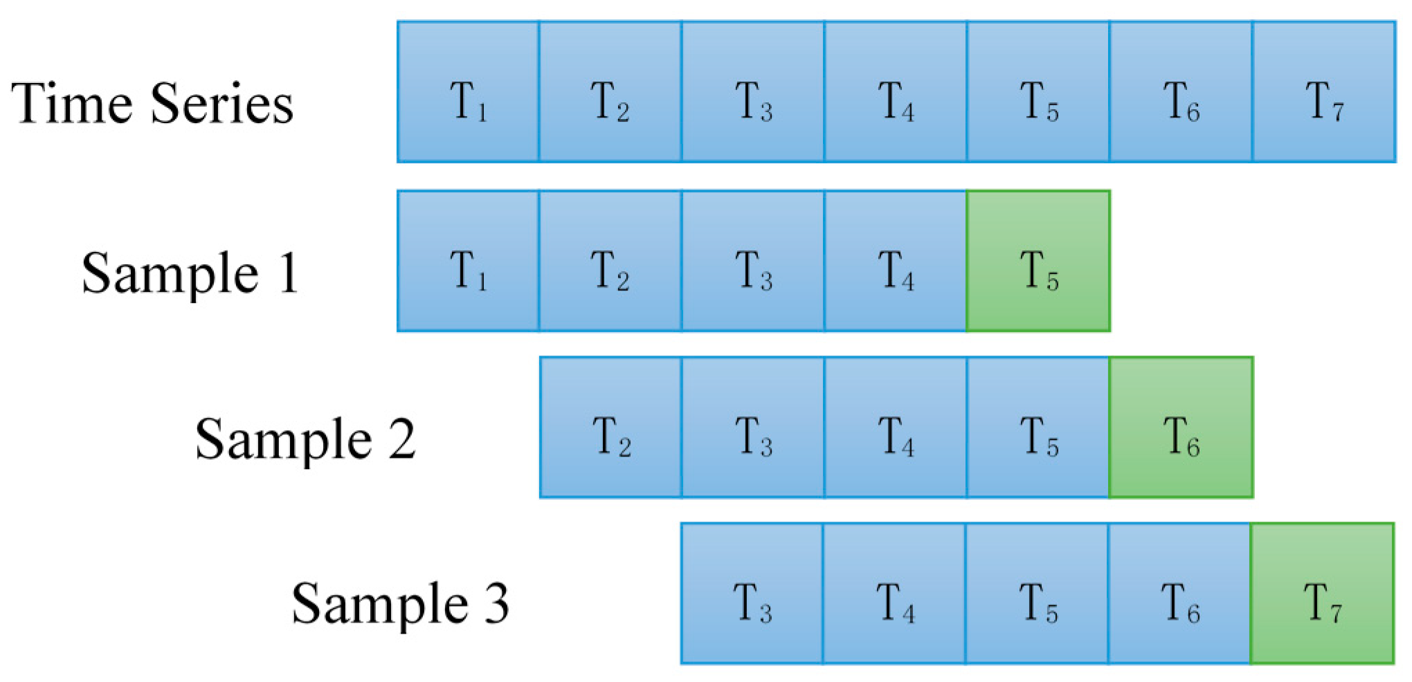
2.1. Sliding Window

The sliding window [20] constructs one sample for each time recording unit T. The samples of T_n use the values within [T_n__p, T_n) as features and the values at T_n as labels or targets, p is called the sliding window size. A sample plot of the sliding window construction time series is shown in Figure 1. T₁ to T₆ are the original time series inputs, and the size of the sliding window is set to 5. Sample 1 features four data from T₁ to T₄, and T₅ is the label of sample 1. Sample 2 features four data from T₂ to T₅, T₆ is the label of sample 2, and so on, the original data of length 9 can build five time series samples. It can be seen that the value of the window size affects the number of time series samples and the features in the samples. For a given data set, a smaller window size means more samples and fewer features; a larger window size means fewer samples and more features.

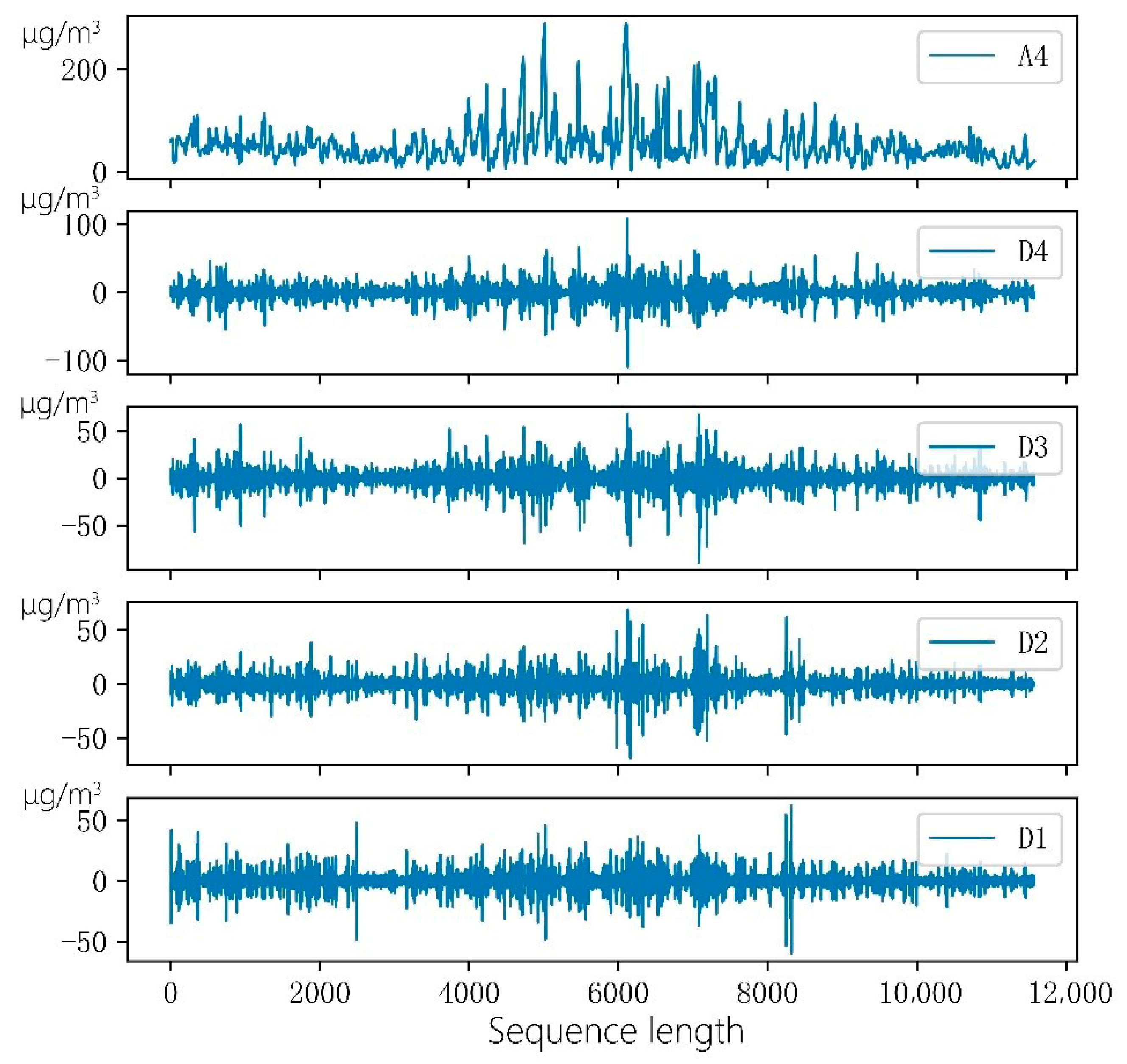
2.2. Wavelet Decomposition

In this paper, we use wavelet decomposition technique to process the raw air quality time series data, which can separate the high-frequency signal with high-frequency detail characteristics from the trending low-frequency signal, so as to obtain more data features. The decomposition process is as follows:

$$\{\begin{array}{l}{A}_{j+1}=H\left(A_j\right)\hfill \\ D_{j+1}=G\left(D_j\right)\hfill \end{array}$$

(1)

where $A_j$, $D_j$ refer to the low-frequency approximation component and the high-frequency detail component, respectively. $H$ is the low-pass filter and $G$ is the high-pass filter. Each layer of the decomposed signal in the process of performing wavelet transform is half of the pre-decomposed signal data, so two interpolation reconstructions are needed to recover the signal length, and the reconstruction formula is as follows:

$$\{\begin{array}{l}{A}_J={\left(H_2\right)}^j{A}_j\hfill \\ D_J={\left(H_2\right)}^{j-1}{G}_2{D}_j\hfill \end{array}$$

(2)

where, $H_2$ and $G_2$ are the dual operators that are $H$ and $G$, respectively. In this paper, a four-layer decomposition followed by reconstruction is performed using the db4 wavelet fundamental to obtain a total of four high-frequency detail components of $D_1$, $D_2$, $D_3$, $D_4$ and one low-frequency approximation component of $A_4$. Figure 2 shows the results of the wavelet decomposition of PM2.5 for the supply and marketing agency. It can be seen that the A₄ low-frequency series has obvious trend as well as certain periodicity, and D_1–4 reflects the random fluctuation changes in the trend of the original time series.

2.3. Complete Ensemble Empirical Mode Decomposition with Adaptive Noise (CEEMDAN)

Compared with empirical mode decomposition (EMD) and ensemble empirical mode decomposition (EEMD), CEEMDAN [21] has better and stronger signal decomposition by overcoming mode mixing, and the eigenmode function of CEEMADN is more favorable for feature extraction. As an optimization of EMD and EEMD algorithms, CEEMDAN can decompose complex raw signals into sequences of IMFs.

2.4. Autoregressive Moving Average Model

The ARMA model is a forecasting model based on stochastic theory that performs model analysis on the perturbation terms so that the model integrates past values, present values and errors, and has high accuracy in smooth stochastic series forecasting [22]. Therefore, in this paper, the ARMA model is used to predict the low-frequency approximate component signals from wavelet decomposition, and the mathematical model of the ARMA model [23] is shown below:

$$\{\begin{array}{l}{A}_J={\phi }_0+{\phi }_1{A}_{J-1}+\cdots +{\phi }_p{A}_{J-p}+{\epsilon }_J-{\theta }_1{\epsilon }_{j-1}-\cdots -{\theta }_q{\epsilon }_{J-q}\hfill \\ {\phi }_p\ne 0,{\theta }_q\ne 0\hfill \\ E\left({\epsilon }_J\right)=0,Var\left({\epsilon }_J\right)={\sigma }_{\epsilon }^2,E\left({\epsilon }_J{\epsilon }_S\right)=0,S\ne J\hfill \\ E\left({\epsilon }_J{\epsilon }_S\right)=0,\forall S<J\hfill \end{array}$$

(3)

where $A_J$ is the input data, 𝜑 is the coefficient of the autoregressive model, 𝜑₀ is a constant, $\theta$ is the moving average model coefficient, ${\epsilon }_J$ is the white noise process, and p and q are the orders of the ARMA model. p refers to the number of lagged observations included in the model. q refers to the size of the moving average window, which is usually used to limit the window size of the sliding window.

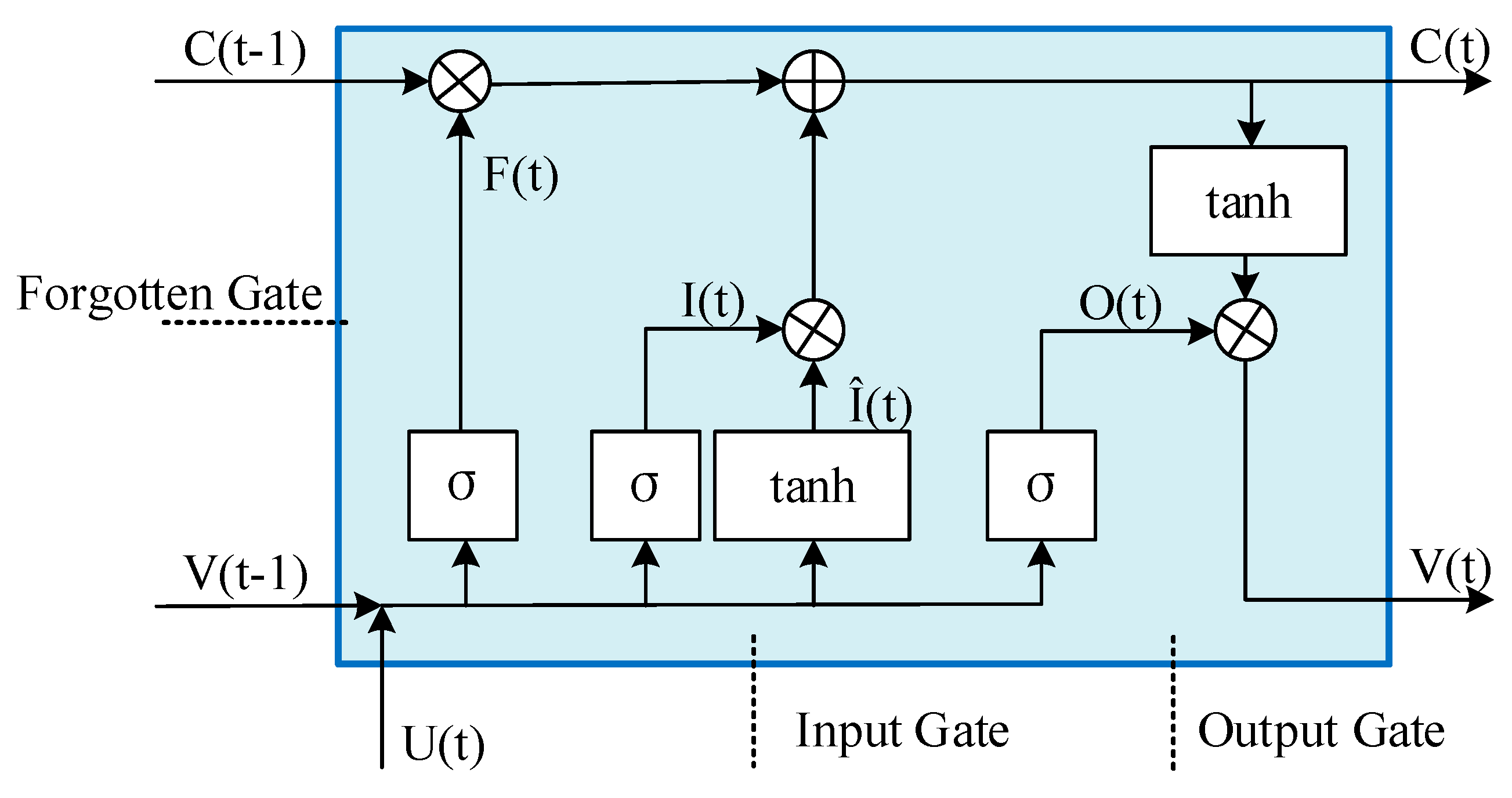
2.5. Long Short-Term Memory

LSTM artificial neural network [24] is a special type of recurrent neural network that is capable of learning long-term dependencies. Even for the longest sequential data, LSTM can avoid gradient disappearance or gradient explosion, and it is widely used to solve sequential data problems such as automatic speech recognition and natural language processing. As shown in Figure 3, LSTM has a complex recursive structure connected in time order, LSTM has two important properties, one is the hidden layer state $V(T)$ that changes with time, and the other is the cell state $C(T)$ that maintains long-term memory. The cell state $C(T)$ is determined by the input gate $I(T)$, forgotten gate $F(T)$ and output gate $O(T)$ at this moment with the hidden layer state $V(T)$ and cell state $C(T)$ at the previous moment; the hidden layer state $V(T)$ is determined by the cell state $C(T)$ and input data at this moment. the updated Equations (4)–(9) for the cell state and hidden layer state in LSTM are as follows:

$$F(t)=\sigma \left(W_f[V(t-1)U(t)]+B_f\right)$$

(4)

$$I(t)=\sigma \left(W_i[V(t-1)U(t)]+B_i\right)$$

(5)

$$O(t)=\sigma \left(W_o[V(t-1)U(t)]+B_o\right)$$

(6)

$$\widehat{I}(t)=\tanh \left(W_i[V(t-1)U(t)]+B_i\right)$$

(7)

$$C(t)=F(t)\cdot C(t-1)+I(t)\cdot \widehat{I}(t)$$

(8)

$$V(t)=O(t)\cdot \tanh (C(t))$$

(9)

where $W$ and $B$ denote the weight matrix and bias vector, respectively, which are obtained by model training; $\sigma$ is the sigmoid activation function and tanh is the tanh activation function. “·” denotes the element-by-element product.

2.6. Predictive Effect Evaluation Index

In this paper, the MAE, RMSE and R² are used to evaluate the prediction accuracy of the model. The MAE reflects the real situation of the error of the prediction value; the RMSE is a measure of the deviation between the prediction value and the actual value, which is more sensitive to the outliers; R² is a statistical measure of the goodness of fit, and the closer its value is to 1, the better the model fits. The expressions are shown below:

$$\mathit{MAE}=\frac{1}{n}\sum _{i=1}^n\left|y-y_{\mathrm{predict}}\right|$$

(10)

$$\mathit{RMSE}=\sqrt{\frac{1}{n}\sum _{i=1}^n{(y-y_{\mathrm{predict}})}^2}$$

(11)

$$R^2=1-\frac{{\displaystyle \sum _{i=1}^n}{(y-y_{\mathrm{predict}})}^2}{{\displaystyle \sum _{i=1}^n}{(y-y_{\mathrm{average}})}^2}$$

(12)

where y is the actual value, $y_{\mathrm{predict}}$ is the predicted value of the model, n is the overall length of the data.

3. Model Construction

3.1. Experimental Environment

The experimental environment is a PC with the following configuration: Windows 10 64-bit, Intel Core i7-7500U CPU@2.70GHz,4GRAM, Using Anaconda Navigator3 (Jupyter notebook), python 3.7 as the experimental platform for simulation.

3.2. Experimental Data

The air quality data used in this thesis are 69,400 data of air quality from six Environmental Protection Bureau (EPB) environmental monitoring stations in Tangshan City, spanning the period from 1 May 2018 to 1 August 2019. The environmental monitoring stations of the EPB sampled air quality-related attributes once every hour.

Table 1. Geographical coordinates of EPB environmental monitoring stations.

Stations	Longitude	Latitude
Gongxiaoshe	118.1662	39.6308
Shierzhong	118.1838	39.65782
Xiaoshan	118.1997	39.6295
Wuziju	118.1853	39.6407
Taocigongsi	118.2185	39.6679
Leidazhan	118.144	39.643

shows the latitude and longitude coordinates of the six EPB environmental monitoring sites in Lubei District, Tangshan.

3.3. Wavelet Decomposition-Long Short Term Memory-Autoregressive Moving Average Prediction Model

The prediction model proposed in this paper is shown in Figure 4, and the specific steps are:

Step 1: The vacant values of all the original data sets are filled by linear interpolation method and the data are min-max normalized, the formula is shown in (13). Then the entire data are decomposed using the fourth-order wavelet transform decomposition and then reconstruction method to obtain four high-frequency signals WD(D) and one low-frequency signal WD(A), and the decomposed results are divided into training set and test set, accounting for 67% and 33% of the total amount, respectively:

$$y_i=\frac{x_i-\underset{1\le j\le n}{\min }\left\{x_j\right\}}{\underset{1\le j\le n}{\max }\left\{x_j\right\}-\underset{1\le j\le n}{\min }\left\{x_j\right\}}$$

(13)

where, $x_i$ represents the original sequence, $n$ represents the length of the sequence, and $y_i$ represents the normalized result.

Step 2: Normalize the training and test sets to obtain the corresponding normalized models.

Step 3: The training set is subjected to ACF and PACF validation, and the length of the sliding window is determined according to the p-value of ACF. The four high-frequency signals WD(D) of the training set after wavelet decomposition are then subjected to sliding window processing by taking the window length of p, respectively, to obtain the two-dimensional input features of the LSTM training model.

Step 4: Input the two-dimensional input features obtained from Step 3 to the built LSTM training model; input the normalized low-frequency signal WD(A) obtained from Step 2 to the ARMA model for training.

Step 5: The data from the test set are input into the trained LSTM and ARMA models to obtain the prediction results, respectively.

Step 6: The final predicted values are generated by overlapping the predicted results of each component.

3.4. Predicted Results

Table 2. The result evaluation of the prediction model.

Stations	Index	AQI	SO2	NO2	CO	O3	PM10	PM2.5
Gongxiaoshe	RMSE	8.9325	3.4657	4.7523	0.2258	8.5855	11.5951	5.9676
	MAE	6.0555	1.9987	3.5679	0.1591	6.3389	7.7954	4.1122
	R2	0.9456	0.9728	0.9501	0.9467	0.9802	0.9525	0.9441
Shierzhong	RMSE	9.28	4.4069	5.1125	0.2962	6.5316	12.4035	6.069
	MAE	6.5033	2.5241	3.7711	0.185	4.8603	8.3986	4.3578
	R2	0.9478	0.9687	0.961	0.9322	0.9872	0.9528	0.9495
Xiaoshan	RMSE	8.7925	4.3061	4.2181	0.2541	6.554	12.9483	5.6387
	MAE	5.911	2.4288	3.1313	0.1516	4.9478	9.1704	4.1039
	R2	0.9506	0.9619	0.9558	0.9285	0.9885	0.9447	0.9523
Wuziju	RMSE	10.4078	4.2532	5.1094	0.2312	5.901	12.7252	5.9236
	MAE	6.8036	2.4893	3.8179	0.1381	4.2853	8.209	4.305
	R2	0.9332	0.9574	0.9508	0.9513	0.9886	0.9578	0.9516
Taocigongsi	RMSE	8.6066	3.1685	4.6597	0.2251	5.9224	12.9119	5.9849
	MAE	5.6633	1.9634	3.4786	0.146	4.4979	8.602	4.2579
	R2	0.9615	0.9735	0.9576	0.9463	0.9886	0.9646	0.9508
Leidazhan	RMSE	8.4232	3.5518	3.4449	0.1732	6.3126	9.7748	5.3129
	MAE	6.0255	2.0302	2.4858	0.1128	4.7903	6.2446	3.8336
	R2	0.9438	0.9666	0.956	0.9712	0.9885	0.9616	0.9498

shows the prediction indicators of the effectiveness of the air quality prediction model proposed in this paper for six air pollutants (SO₂, NO₂, CO, O₃, PM10, PM2.5) and the AQI at six EPB monitoring stations in Tangshan City.

The prediction accuracy of the air quality prediction model proposed in this paper does not differ much in each station, and good prediction results were achieved for both criteria air pollutants and AQI. As can be seen from Table 2, the air quality prediction model proposed in this paper has a good fitting effect, and the value of R² shows that the average index R² of the prediction results of the air quality data from the environmental monitoring stations of other EPBs reaches more than 0.94, except for the prediction results of CO in XII and the AQI of the Bureau of Materials. Therefore, the air quality prediction model WD-LSTM-ARMA proposed in this thesis has a good fitting effect.

4. Comparison and Analysis

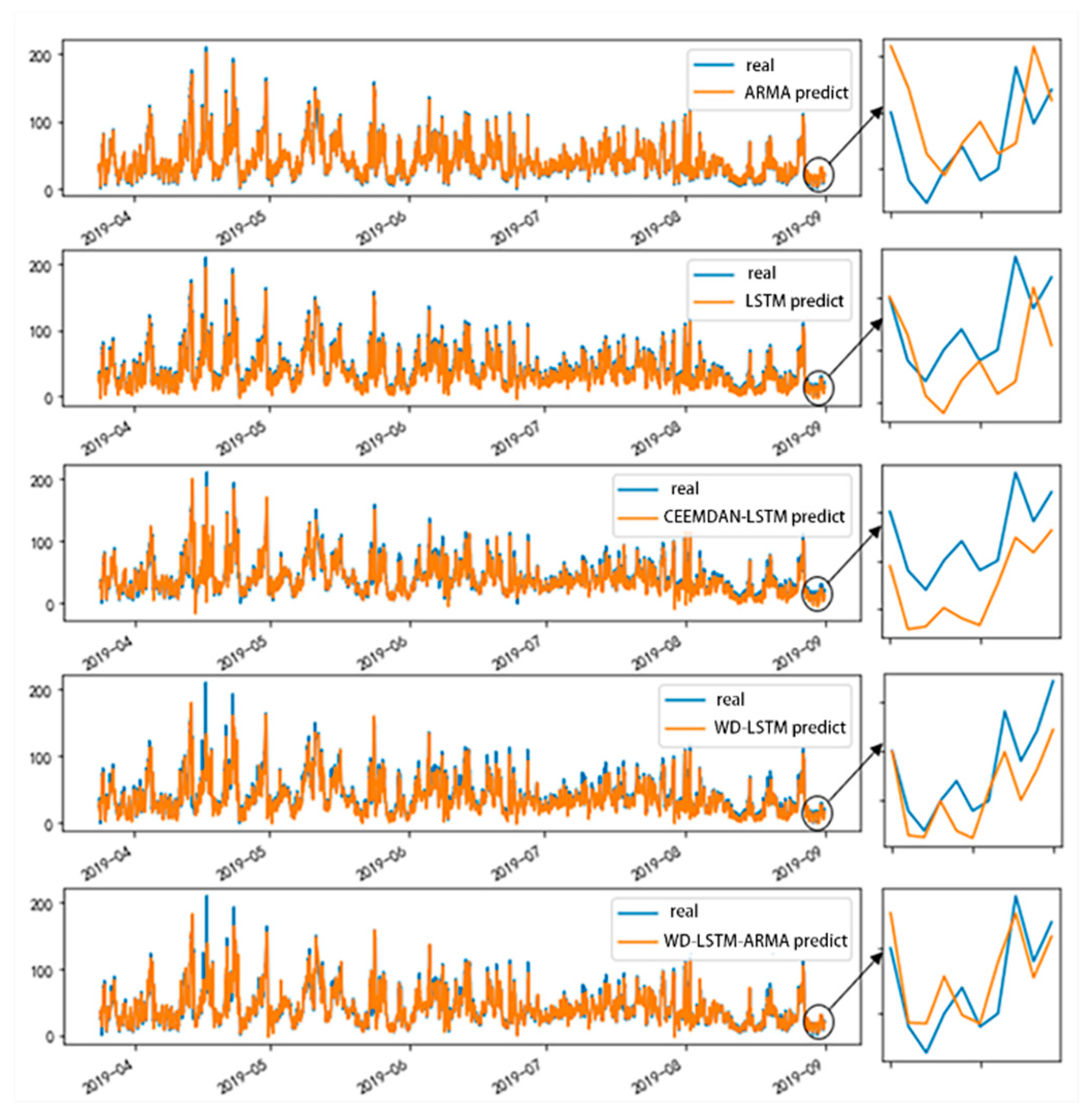
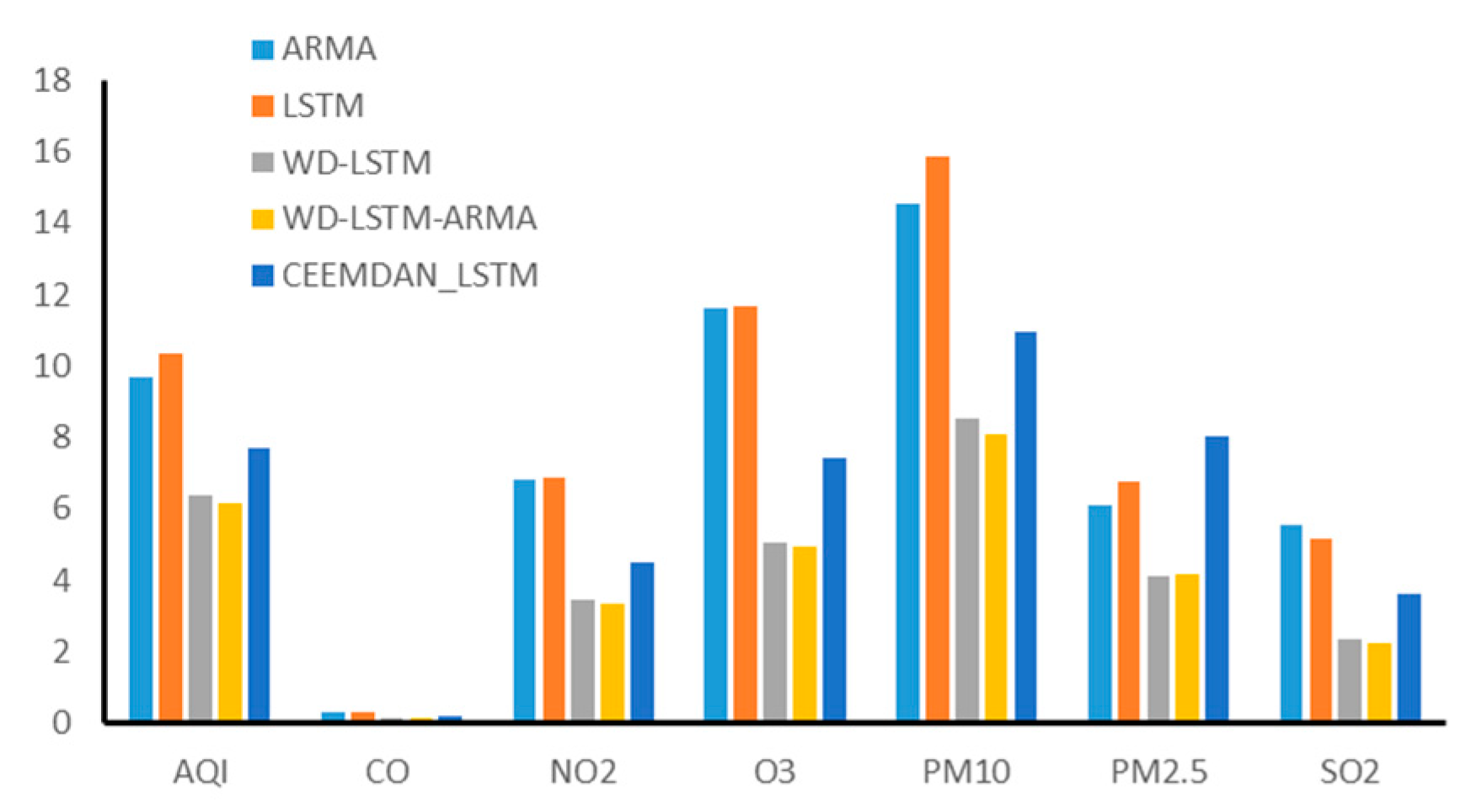
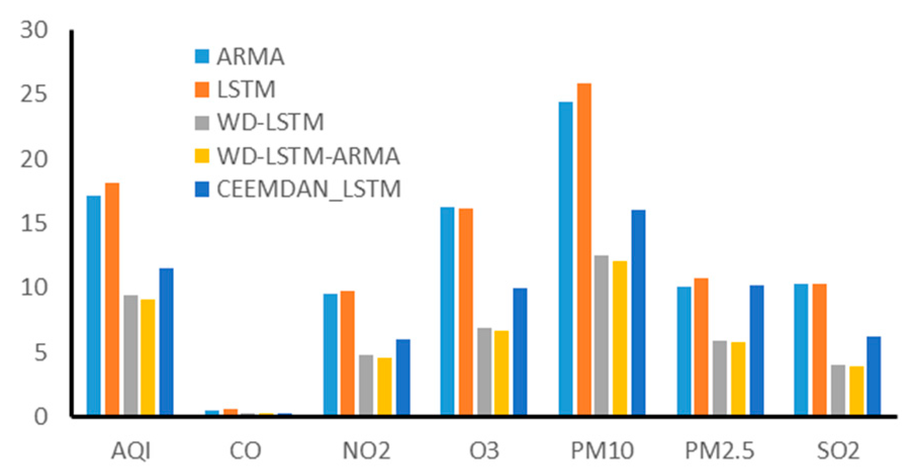
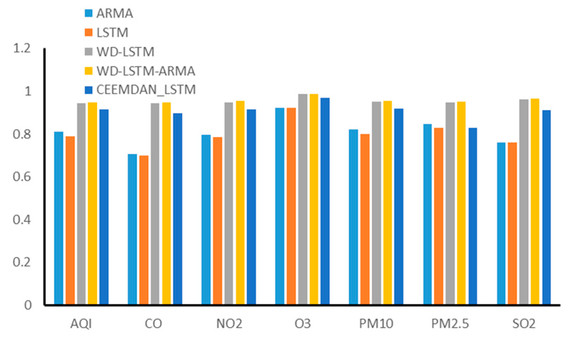
4.1. Model Comparison

In order to verify the validity of the prediction model proposed in this paper, the model proposed in this paper was compared and analyzed with other prediction models. In addition to the prediction models proposed in this paper, four other prediction models were applied, including two single prediction models, LSTM and ARMA, and two hybrid models, CEEMDAN-LSTM and WD-LSTM, respectively. The architecture of these five prediction models is shown in Figure 5. The WD-LSTM prediction model is to send the four high-frequency sequences and one low-frequency sequence obtained from wavelet decomposition into the LSTM prediction model for prediction, and finally the prediction results of each sequence are reconstructed to obtain the final prediction results. the CEEMDAN-LSTM prediction model uses the CEEMDAN decomposition [21] method to the original data is decomposed, and then the decomposed subsequences are sent into the LSTM separately for prediction, and finally the predicted results are reconstructed to obtain the final prediction results.

4.2. Case Analysis

Taking the PM2.5 of Tangshan city supply and marketing agency as a case study, we can see from Figure 6 that the single prediction model LSTM and ARMA model predict the trend of PM2.5 quite well. Because of the autocorrelation of the series, the lag between the predicted and actual values is easy to occur, that is, the predicted value at moment t seems to be obtained by translating the actual value at moment t-1. From the prediction results of the hybrid model, it can be seen that the problem of lagging prediction results that existed in the single model has been eliminated. The prediction accuracy of CEEMDAN-LSTM is improved compared to the single model, but the overall predicted values are smaller than the actual values. Therefore, WD-LSTM and WD-LSTM-ARMA perform relatively well.

Combined with the error box diagram in Figure 7, it can be seen that there are large error points in LSTM and ARAM, and the overall error range is also larger compared to the hybrid prediction model. CEEMDAN-LSTM suffers from most of the predicted values being smaller than the actual values, and there are also large error points relative to WD-LSTM and WD-LSTM-ARMA. WD-LSTM and WD-LSTM-ARMA perform better, but WD-LSTM-ARMA has a more concentrated overall error and the smallest mean absolute error.

The prediction performance of the five prediction algorithms was evaluated by taking the mean values of the evaluation indexes of the prediction effects of the six air pollutants and the AQI from six monitoring stations in Tangshan City. As can be seen from Figure 8, Figure 9 and Figure 10, the single prediction models LSTM and ARMA are not satisfactory in predicting either the six air pollutants or the AQI. Overall, the hybrid model predicted all six air pollutants and AQI better than the single prediction model, with CEEMDAN-LSTM performing worse, indicating that the single CEEMDAN decomposition method was not able to fully extract the effective information of the time series. Although the prediction models of WD-LSTM and WD-LSTM-ARMA have similar prediction performance with similar accuracy in predicting PM2.5 concentrations, WD-LSTM-ARMA is significantly better than WD-LSTM model for other pollutants as well as AQI, and the WD-LSTM-ARMA code has shorter computing time.

Through the overall statistical analysis of the evaluation indexes of the prediction results, the WD-LSTM-ARMA air quality prediction model proposed in this paper reduced the RMSE by 52%, reduced the MAE by 47%, and improved the R² by 18% relative to the single model ARMA with higher prediction accuracy; and reduced the RMSE by 3%, reduced the MAE by 3%, and improved the R² by 0.5% relative to the other hybrid model WD-LSTM with higher prediction accuracy.

5. Conclusions

Since air quality is deteriorating worldwide, accurate air quality prediction has important theoretical and practical significance for production and life. This study proposes a hybrid model for air quality prediction based on data decomposition with a focus on air quality prediction. It is experimentally verified that the WD-LSTM-ARMA air quality time-scale prediction model based on data decomposition proposed in this paper can extract the periodic features as well as the random features of the original time series through wavelet decomposition, which has good prediction accuracy and generalizability and is applicable to the prediction of six pollutants as well as the AQI. By introducing a sliding window to handle high-frequency subsequence data, the information required for the model training process can be satisfied while reducing the collection of other feature data. Comparative experiments are conducted with the single prediction models ARMA and LSTM and the hybrid models CEEMDAN-LSTM and WD-LSTM. The experimental results show that the proposed prediction model WD-LSTM-ARMA is 52% lower on RMSE, 47% lower on MAE, and 18% higher on R² compared to the single model. WD-LSTM-ARMA is 3% lower on RMSE, 3% lower on MAE, and 0.5% higher on R² compared to the hybrid model. Therefore, the model is more suitable for prediction of air quality.

For the future demand of air pollution control and even urban construction for air quality prediction, the model proposed in this paper can be subsequently integrated with decomposition methods or time series problems in anticipation of better prediction results, and it can also be applied to gas load prediction, short-term prediction of network traffic flow and short-term power load prediction.

References

1. Zhao, G.; Huang, G.; He, H.; He, H.; Ren, J. Regional Spatiotemporal Collaborative Prediction Model for Air Quality. IEEE Access 2019, 7, 134903–134919. [Google Scholar] [CrossRef]
2. Zheng, H.; Cheng, Y.; Li, H. Investigation of Model Ensemble for Fine-Grained Air Quality Prediction. China Commun. 2020, 17, 207–223. [Google Scholar] [CrossRef]
3. Li, W.; Lu, C.; Ding, Y. A Systematic Simulating Assessment WithinReach Greenhouse Gas Target by Reducing PM2.5Concentrations in China. Pol. J. Environ. Stud. 2017, 26, 683–698. [Google Scholar] [CrossRef]
4. Filipiak-Florkiewicz, A.; Topolska, K.; Florkiewicz, A.; Cieślik, E. Are Environmental Contaminants Responsiblefor ‘Globesity’? Pol. J. Environ. Stud. 2017, 26, 467–478. [Google Scholar] [CrossRef]
5. Mahmood, S.; Ali, S.; Qamar, M.A.; Ashraf, M.R.; Atif, M.; Iqbal, M.; Hussain, T. Hard Water and Dyeing Properties:Effect of Pre- and Post-Mordanting on DyeingUsing Eucalyptus Globulus AndCurcuma Longa Extracts. Pol. J. Environ. Stud. 2017, 26, 747–753. [Google Scholar] [CrossRef]
6. Liu, H.; Li, Q.; Yu, D.; Gu, Y. Air Quality Index and Air Pollutant Concentration Prediction Based on Machine Learning Algorithms. Appl. Sci. 2019, 9, 4069. [Google Scholar] [CrossRef] [Green Version]
7. Appel, K.W.; Pouliot, G.A.; Simon, H.; Sarwar, G.; Pye, H.O.T.; Napelenok, S.L.; Akhtar, F.; Roselle, S.J. Evaluation of Dust and Trace Metal Estimates from the Community Multiscale Air Quality (CMAQ) Model Version 5.0; Atmospheric Sciences: Leeds, UK, 2013. [Google Scholar]
8. Woody, M.C.; Wong, H.-W.; West, J.J.; Arunachalam, S. Multiscale Predictions of Aviation-Attributable PM2.5 for U.S. Airports Modeled Using CMAQ with Plume-in-Grid and an Aircraft-Specific 1-D Emission Model. Atmos. Environ. 2016, 147, 384–394. [Google Scholar] [CrossRef]
9. Donnelly, A.; Misstear, B.; Broderick, B. Real Time Air Quality Forecasting Using Integrated Parametric and Non-Parametric Regression Techniques. Atmos. Environ. 2015, 103, 53–65. [Google Scholar] [CrossRef]
10. Jin, X.-B.; Yang, N.-X.; Wang, X.-Y.; Bai, Y.-T.; Su, T.-L.; Kong, J.-L. Deep Hybrid Model Based on EMD with Classification by Frequency Characteristics for Long-Term Air Quality Prediction. Mathematics 2020, 8, 214. [Google Scholar] [CrossRef] [Green Version]
11. Wu, Q.; Lin, H. A Novel Optimal-Hybrid Model for Daily Air Quality Index Prediction Considering Air Pollutant Factors. Sci. Total Environ. 2019, 683, 808–821. [Google Scholar] [CrossRef] [PubMed]
12. Salazar, L.; Nicolis, O.; Ruggeri, F.; Kisel’ák, J.; Stehlík, M. Predicting Hourly Ozone Concentrations Using Wavelets and ARIMA Models. Neural Comput. Appl. 2019, 31, 4331–4340. [Google Scholar] [CrossRef] [Green Version]
13. Mallat, S.G. Multifrequency Channel Decompositions of Images and Wavelet Models. IEEE Trans. Acoust. Speech Signal Process. 1989, 37, 2091–2110. [Google Scholar] [CrossRef] [Green Version]
14. Jiang, F.; He, J.; Tian, T. A Clustering-Based Ensemble Approach with Improved Pigeon-Inspired Optimization and Extreme Learning Machine for Air Quality Prediction. Appl. Soft Comput. 2019, 85, 105827. [Google Scholar] [CrossRef]
15. Cabaneros, S.M.; Calautit, J.K.; Hughes, B. Spatial Estimation of Outdoor NO2 Levels in Central London Using Deep Neural Networks and a Wavelet Decomposition Technique. Ecol. Modell. 2020, 424, 109017. [Google Scholar] [CrossRef]
16. Liu, H.; Chen, C. Spatial Air Quality Index Prediction Model Based on Decomposition, Adaptive Boosting, and Three-Stage Feature Selection: A Case Study in China. J. Clean. Prod. 2020, 265, 121777. [Google Scholar] [CrossRef]
17. Wang, D.; Wei, S.; Luo, H.; Yue, C.; Grunder, O. A Novel Hybrid Model for Air Quality Index Forecasting Based on Two-Phase Decomposition Technique and Modified Extreme Learning Machine. Sci. Total Environ. 2017, 580, 719–733. [Google Scholar] [CrossRef] [PubMed]
18. Zhang, Z.; Zeng, Y.; Yan, K. A Hybrid Deep Learning Technology for PM2.5 Air Quality Forecasting. Environ. Sci. Pollut. Res. 2021. [Google Scholar] [CrossRef]
19. Wu, C.-H.; Lu, C.-C.; Ma, Y.-F.; Lu, R.-S. A New Forecasting Framework for Bitcoin Price with LSTM. In Proceedings of the 2018 IEEE International Conference on Data Mining Workshops (ICDMW), Singapore, 17–20 November 2018; IEEE: Piscataway, NJ, USA, 2018; pp. 168–175. [Google Scholar]
20. Ma, J.; Ding, Y.; Gan, V.J.L.; Lin, C.; Wan, Z. Spatiotemporal Prediction of PM2.5 Concentrations at Different Time Granularities Using IDW-BLSTM. IEEE Access 2019, 7, 107897–107907. [Google Scholar] [CrossRef]
21. Liu, Y.; Wang, L. Drought Prediction Method Based on an Improved CEEMDAN-QR-BL Model. IEEE Access 2021, 9, 6050–6062. [Google Scholar] [CrossRef]
22. Velasco, C.; Lobato, I.N. Frequency Domain Minimum Distance Inference for Possibly Noninvertible and Noncausal ARMA Models. Ann. Statist. 2018, 46. [Google Scholar] [CrossRef]
23. Lennon, H.; Yuan, J. Estimation of a Digitised Gaussian ARMA Model by Monte Carlo Expectation Maximisation. Comput. Stat. Data Anal. 2019, 133, 277–284. [Google Scholar] [CrossRef] [Green Version]
24. Graves, A. Long Short-Term Memory. In Supervised Sequence Labelling with Recurrent Neural Networks; Studies in Computational Intelligence; Springer: Berlin/Heidelberg, Germany, 2012; Volume 385, pp. 37–45. ISBN 978-3-642-24796-5. [Google Scholar]
Figure 1. Sliding Window.
Information 12 00210 g001
Figure 2. Results of wavelet decomposition.
Information 12 00210 g002
Figure 3. LSTM network structure.
Information 12 00210 g003
Figure 4. WD-LSTM-ARMA algorithm block diagram.
Information 12 00210 g004
Figure 5. Analytical comparison model.
Information 12 00210 g005
Figure 6. Model prediction results.
Information 12 00210 g006
Figure 7. Error box diagram.
Information 12 00210 g007
Figure 8. The MAE histogram of prediction results for each model.
Information 12 00210 g008
Figure 9. The RMSE histogram of prediction results for each model.
Information 12 00210 g009
Figure 10. The R2 histogram of prediction results for each model.
Information 12 00210 g010