Abstract
Heart sounds play an important role in the initial screening of heart diseases. However, the accurate diagnosis with heart sound signals requires doctors to have many years of clinical experience and relevant professional knowledge. In this study, we proposed an end-to-end lightweight neural network model that does not require heart sound segmentation and has very few parameters. We segmented the original heart sound signal and performed a short-time Fourier transform (STFT) to obtain the frequency domain features. These features were sent to the improved two-dimensional convolutional neural network (CNN) model for features learning and classification. Considering the imbalance of positive and negative samples, we introduced FocalLoss as the loss function, verified our network model with multiple random verifications, and, hence, obtained a better classification result. Our main purpose is to design a lightweight network structure that is easy for hardware implementation. Compared with the results of the latest literature, our model only uses 4.29 K parameters, which is 1/10 of the size of the state-of-the-art work.
1. Introduction
According to statistics from the World Health Organization, cardiovascular disease has become one of the leading causes of death in the world [1]. Effective monitoring and testing methods can increase the number of groups screened and therefore reduce mortality. The first step in evaluating cardiovascular disease in clinical practice is a physical examination. Auscultation of heart sounds is an important part of the physical examination. During the cardiac cycle, the heart undergoes electrical stimulation, and the formation of atrial and ventricular contractions leads to mechanical activity. This mechanical activity, as well as the sudden starting or stopping of blood flow in the heart, will cause the entire heart structure to vibrate. These vibrations can be heard on the chest wall, and specific heart sounds can give an indication of heart health [2]. As an important initial screening method, heart sound diagnosis can uncover many pathological heart diseases, such as heart rate failure, valvular disease, heart failure, and so on [2,3]. However, traditional heart sound auscultation methods are highly dependent on the experience of the doctor. Only doctors with many years of experience can accurately diagnose whether a patient may have heart disease with this method. Hence, auscultation is not suitable for situations where there are limited medical resources and a large patient population, such as occurs in general practice. Therefore, it is necessary to investigate a method for automatically classifying heart sounds that can be applied to develop a portable low-power automatic monitoring device.
The method of heart sound classification usually involves three main steps: feature extraction, feature selection, and feature classification. The accuracy of heart sound classification is greatly affected by the three steps. Many scholars have conducted related research on automatic classification technology for heart sounds. The first group of researchers, who studied the threshold method for automatic heart sound classification [4], proposed using a computer to process the phonocardiogram (PCG). A method of using multi-threshold features and support vector machines (SVMs) to classify normal and abnormal heart sounds has also been proposed [5]. This classifier achieves a good overall accuracy (86.8%), but the process of feature extraction is much too complicated. In recent years, the neural network model has shown excellent performance in data prediction and solving various classification problems. It can be applied to the automatic diagnosis of heart sounds to classify diseases well. Another study has reported combining SVM with a discrete wavelet transform (DWT) and Mel-frequency cepstral coefficients (MFCCs) features, the K-nearest neighbor (KNN) algorithm based on centroid displacement, and classification algorithms based on deep neural networks (DNNs) to classify heart sounds [6]. The classification accuracy of this algorithm is high (97%), but the model is very complicated and requires extensive calculations. Other researchers focused on various strategies for feature extraction based on the convolutional neural network (CNN) method and showed that the CNN-based method has a higher classification accuracy [7,8,9,10,11] (91%, 89.22%, 96.33%, 98%, 81.5% respectively). These methods show that complicated manual feature extraction combined with CNN network model can obtain good classification accuracy, but it is difficult to achieve low power consumption in mobile devices. In another approach, a method of heart sound diagnosis without segmentation was introduced [12]. This method uses fast Fourier transform and wavelet analysis to extract corresponding frequency features, and decision trees as feature classifiers. It was proved that, in the case of poor signal quality, an accuracy rate (80%) equivalent to other methods could be obtained without segmentation of the heart sounds.
Among the above algorithms for automatic heart sound recognition, many involve a multi-threshold feature extraction process and a complex calculation process, and then apply machine learning methods or multilayer neural network models for feature recognition and classification. However, these network models are relatively complex and they require large amounts of calculations, so they are not suitable for integration into low-power mobile monitoring equipment. Here, we developed a lightweight heart sound automatic classification model that does not require heart sound segmentation. The model only uses frequency-domain feature input, which is sent to an improved two-dimensional CNN for training and classification. The model was tested on the 2016 PhysioNet dataset and obtained an average accuracy of 86%, which greatly reduced the calculation parameters of the model while maintaining a high accuracy rate. Hence, the proposed system provides an excellent classification performance. Our focus was to build a stable and reliable lightweight classification model by improving the classic CNN network structure, introducing a weighted loss function (FocalLoss [13]) to alleviate the unbalanced positive/negative portions in our samples, and optimizing all parameters. The main outstanding contributions of this paper are as follows:
(i) By adjusting the parameters and structure of the short-time Fourier transform (STFT) and CNN, the complexity of the model was greatly simplified, better model parameters were obtained, and relatively high accuracy was achieved.
(ii) The convergence of the data was sped up by adding the batch normalization [14] module, and the imbalance of the sample was solved by adding the FocalLoss loss function. At the same time, we designed a very simple CNN network that only has 1/10 of the parameters of the state-of-the-artwork.
2. Materials and Methods
2.1. Dataset
Before the PhysioNet/CinC Challenge 2016, only three public heart sound databases were available: (1) Michigan Heart Sounds and Murmur Database (UMHS) [15], (2) Pascal Database (Bentley et al., 2011) [16], and (3) Heart Auscultation Heart Murmur Database (EGeneralMedical) [17]. However, the quality of these databases is greatly affected by the number of records, length and frequency of signals, and the noise in the signals. In this study, the database and annotations that we used are from the public PhysioNet Cardiology Challenge 2016 [2]. This database comes from eight independent databases contributed by seven research groups and is currently the largest available heart sound database marked by experts in the field. These databases are divided into two large parts, the training set and the test set (unpublished). The numbers of labels for positive and negative samples in the training sets are shown in Figure 1.
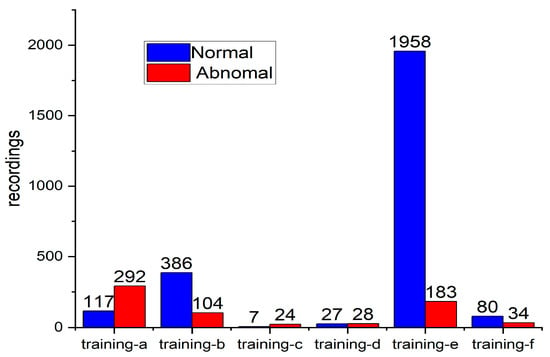
Figure 1.
Normal and abnormal samples in each training set.
From Figure 1, the number of records of normal and abnormal signals in these databases is very unbalanced, and the imbalance in the samples in the training-e set is the most significant. We therefore used a weighted loss function in feature training to balance our positive and negative samples, making our results more reliable, which will be introduced in more detail in the feature classification section. In addition, because this database was prepared for a competition, the training set data were the only data we had access to, and the test set data were used as a hidden dataset to compile the official test score. Hence, this experiment was conducted on the public training dataset.
As shown in Figure 2, the network model that we propose in the following includes three parts: feature extraction, feature classification, and test verification. We also focused on the improvement of the network structure, the adjustment of model parameters, and the treatment of imbalanced data.
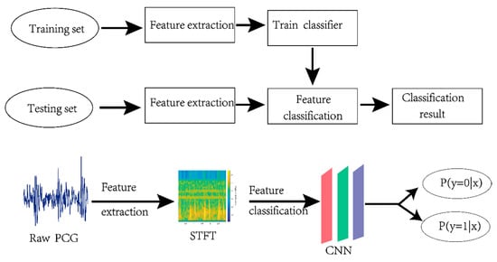
Figure 2.
Block diagram of our proposed network model. Firstly, we preprocessed and segmented the heart sound data. Then, we extracted the features in the frequency domain. Finally, we sent the features to the convolutional neural network (CNN) model that we designed to classify normal and abnormal heart sounds.
2.2. Feature Extraction
Since the signal at the recording level is more susceptible to interference from clutter than the signal at the slice level, the segmentation method usually has stronger robustness against noise in the environment during acquisition or transmission. Since the phonocardiogram (PCG) classification aims to give the predicted category of each PCG record, we introduced a fixed-length segmentation using overlapping windows. Firstly, we filtered the original signal with a 10-Hz high-pass filter. The duration of the heart sound cycle is usually 0.6–1 s, so we divided the filtered heart sound signal into small segments of 3 s (if the last segment was less than 3 s, it was omitted), and the step length of each jump was 1.5 s, which ensured that there would be at least one complete heart sound cycle signal in each segment, as shown in Figure 3.
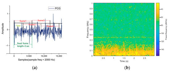
Figure 3.
Segmentation of the heart sound signal and a time-frequency diagram of a 3 s segment. (a) Asynchronous segmentation example with a length of 3 s where the hop size was 1.5 s. (b) Time-frequency diagram of the heart sound signal of 3 s.
We used STFT to extract frequency domain information for each small segmented signal, and Hamming windows with different window lengths and overlap rates to segment the signal. The parameters of the model (n_fft = 150, hop_length = 75, win_length = 150) leading to a better classification effect were selected based on the overall accuracy rate. Under these parameters, we obtained the size of the two-dimensional feature map of each 3-s signal to 76 × 79, as shown in Figure 3. We then obtained the two-dimensional time-frequency graph matrix of each segmented signal, as shown in Figure 3b, and sent it to the CNN training classifier that we designed for training and classification.
2.3. Feature Classification
In the process of feature classification, due to the complexity of heart sound signals, it was necessary to synthesize the information of one or more cycles of heart sound signals in the feature extraction in order to improve the classification capability at each time point. These heart sound signals had a large number of features, which meant that the algorithm of feature classification became very complicated. Currently, CNNs and recurrent neural networks (RNNs) are the mainstream algorithms used in the study of heart sound signal classification because their multi-layer networks can better fit complex functions [18] and they usually have better classification capabilities. However, their numbers of parameters and calculations are relatively large. To take advantage of the powerful learning ability of CNN, we used a three-layer CNN network model to classify features. Compared with traditional networks, this network model was simpler and it was able to adapt to become compatible with input features of different sizes. The model structure of the improved CNN is shown in Figure 4.

Figure 4.
Block diagram of the CNN model proposed.
As shown in Figure 4, a three-layer two-dimensional CNN network for feature learning and classification was adopted firstly. The size of the input to the two-dimensional-feature model was 79 76. Then, filters were used to extract the features of each layer, and the maximum pooling was used to reduce the parameters of the subsequent fully-connected layer and realize adaptability to different sizes of the input matrix. Finally, through the SoftMax layer, the probabilities of predictions of 1 and 0 were obtained, among which the higher probability was the prediction category of the sample.
Compared with the traditional CNN network, our model made the following improvements:
- The pooling layer after each layer of convolution was removed, and a batch normalization module was introduced before the activation function of Relu, which normalized the model of each layer [14]. The added batch normalization module is
- where is the original activation function of a certain neuron, and are the mean value and standard deviation of the input neuron, is the expansion factor, is the translation factor, and is the normalized value. Formula (1) normalizes the convolution result to a standard normal distribution with a mean of 0 and a variance of 1 and then performs the corresponding scaling and shifting operations. This operation ensures that the input of each layer of the neural network retains the same distribution, which can alleviate the gradient explosion and disappearance phenomena that may perturb the propagation process, and help the model converge faster.
- Before the fully connected layer, the maximum pooling layer was introduced, which can greatly reduce the quantity of parameters of the fully connected layer. As a result, the 9520 parameters before maximum pooling were reduced to only 8 parameters after maximum pooling, which greatly simplified the optimization parameters of the fully connected layer.
- The entire model only used a 3-layer CNN network, a maximum pooling layer, and a fully connected layer to output the results, which is a very light structure in the application of heart sound classification.
2.4. Solving the Problem of Unbalanced Classification
For the binary classification task, in the usual CNN network, the feature nodes generated by the fully connected layer are fed to the classification layer to output the probability. Usually, in the loss of the model calculation, each category has the same loss weight by default. However, when performing classification tasks with unbalanced samples, this may make the results of the prediction model extremely unbalanced. In many clinical datasets, the number of positive samples is far greater than the number of negative samples. If the method of balancing the samples is not adopted, the prediction result will make the accuracy of negative samples very low and the accuracy of the prediction results of positive samples high. Therefore, in this experiment, we adopted FocalLoss as the loss function of our model [13]. This model applies different penalties to mispredicted categories and defines new weights for each category. The loss function is
where can be used to balance the importance of positive and negative samples and is used to adjust the rate of weight reduction of simple samples. Experiments have found that a value of 2 is the best [13]. In Formula (2), the greater the probability of sample misclassification, the greater the probability of its loss function, and the greater the penalty for small sample misclassification through α adjustment. A greater probability of sample misclassification causes an increase in the probability of its loss function and results in a rising penalty for small sample misclassification through α adjustment.
2.5. Evaluation of Results
In the last layer of the CNN, we used Softmax to predict the results of the probability values of 0 (normal) and 1 (abnormal). If the predicted probability of 1 was greater than that of 0, we marked the predicted label of this small segment (of 3 s) as 1; otherwise, it was 0. We then used Formula (3)
to mark the label of the entire signal.
In Formula (3), we counted the proportion of the segment marked as 1 to the entire segment entry of the heart sound signal. When it was greater than our threshold, the entire heart sound signal was marked as 1 (abnormal); otherwise, it was marked as 0 (normal).
In order to evaluate the accuracy of the results, we used sensitivity, specificity, MACC (mean accuracy, the mean value of sensitivity and specificity) and ACC (accuracy, the proportion of the correct samples to the entire sample). The formulas are as follows:
Sensitivity:
Specificity:
MACC:
ACC:
where TP, TN, FP, and FN represent the number of true positive, true negative, false positive, and false negative samples, respectively, in a certain experiment.
3. Results
In this experiment, we used TensorFlow to build our network structure. For each segment of the signal, we first let the signal pass through a 10-Hz high-pass filter. Then, we took 20% of the data in the a, b, c, d, e, and f datasets as the fixed test set, and randomly divided the remaining data into a training set (60%) and a validation set (20%). Then, we divided each entire segment of the signal into small segments of 3 s, overlapping each time by 1.5 s, and if the final segment was less than 3 s, it was discarded. The window of each small segment of the signal (3 s) was used for each STFT computation, and the two-dimensional features obtained were sent to the CNN network model for training and classification. In the experiment, we determined the final model parameters according to the validation set of the highest accuracy by conducting multiple random tests on the length of the window of the STFT, the parameters of the FocalLoss function, and the output threshold. The remaining 80% of the data was randomly divided into a training set (60%) and a validation set (20%) and the random division was repeated 6 times. The 6 training models were thereby obtained and the corresponding results for accuracy were acquired by using the training models on the test set.
3.1. The Effects of STFTs with Different Window Lengths on Accuracy
STFTs with different window lengths have different resolutions in the time domain and frequency domain. In order to obtain a relatively high accuracy rate, in the course of the experiment, we carried out multiple experiments on different window lengths. We found that, when the window length was 150 and the overlap rate was 50%, the ACC of the classification result was the highest, as shown in Figure 5.
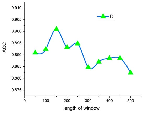
Figure 5.
Influence of short-time Fourier transforms (STFTs) with different window lengths on ACC.
3.2. Influence of the Different Weights of the Loss Function and the Final Threshold on the Results
In the training process, to balance Sn and Sp as much as possible, we set different classification weights through the loss function to solve the classification imbalance and improve the MACC of the classifier. We set the classification weight and the threshold to different values, which varied from 0.1 to 0.5, and trained the model with the prepared training and validation sets. The optimal parameters of the validation set were used for the parameters of the final model, and the corresponding test results were obtained. We also tested the impact of different classification thresholds on the results, as shown in Figure 6.
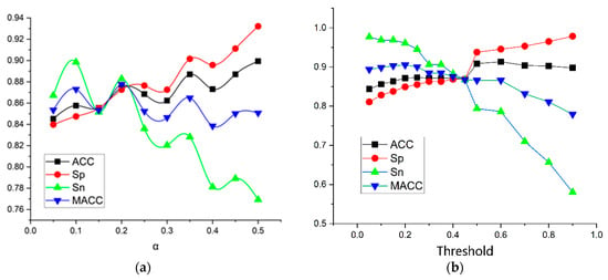
Figure 6.
Impacts of different weights () and thresholds on the classification results. (a) Effects of different weights on the classification results. (b) Impacts of different thresholds on the accuracy of the results.
As seen in Figure 6, when the FocalLoss value was about 0.2 and the classification threshold value was about 0.45, the values of ACC and MACC were relatively high, and Sn and Sp were not very different, indicating that the balance between the positive and negative samples was optimized and thus the model had the best generalization capability.
Table 1 shows the statistical results when α was set to 0.2 and 0.5, meaning with and without classification weight, respectively. It can be seen that the MACC obtained with classification weight was 2% higher than the default average loss function. The default weight of Sn was very low, indicating that the classification accuracy of abnormal samples was low. This does not meet our daily requirements for disease classification in that the abnormal samples should be sensed with high accuracy. In general, when α = 0.2 and = 0.5, ACC was higher, but the results for this statistic were extremely unbalanced. The positive samples occupied the largest proportion, so it was not reliable to use ACC alone to evaluate the classification capability. The weighted loss function that we proposed not only alleviated the impacts of the imbalance of positive and negative samples, but also had higher MACC and ACC and better classification capabilities.

Table 1.
Comparison of classification performance with weight (α = 0.2) and without weight (α = 0.5).
3.3. Classification Performance for Normal and Abnormal Heart Sounds
Based on all of the above test results, we set the corresponding optimal hyperparameters via the 6 random values for training and testing on the test set. The results of the 6 tests were obtained and corresponding statistics were calculated for the results, as shown in Table 2.

Table 2.
Results and statistics verified by 6 experiments (%).
Our results were robust with stable means and standard deviations across the 6 experiments, although the fluctuations of Sn and Sp were slightly large, which is due to the imbalance of the data.
4. Discussion
In this research, we proposed a lightweight method for automatic heart sound recognition. This method used the characteristics of frequency domain signals and an improved end-to-end CNN model to achieve a higher accuracy classification of heart sounds. Meanwhile, we directly segmented the PCG signal instead of using the official recommended feature extraction method of dividing the heart sound cycle (s1-systolic-s2-diastolic). Using frequency domain signal extraction, it was sent to the CNN model that we designed for classification. By modifying the model structure and continuously adjusting the model parameters, we obtained the optimal parameter setting for the model. This method does not require the previous process involving a large number of manual feature extractions, which greatly reduced the amount of calculation and avoided multiple feature redundancy, and an unnecessary calculation burden. The batch normalization module was introduced to speed up the convergence of the model. Maximum pooling was used before the fully connected layer, which greatly reduced the number of parameters and avoided overfitting of the model. It also improved the accuracy of the model. In addition, we introduced the FocalLoss function with weight classification as the loss function, which solved the imbalance problem of positive and negative samples and made the results of the model more credible.
We compared our results with the results of the challenge and the most recent literatures, as shown in Table 3.

Table 3.
Comparison of results among different methods (%).
In Table 3, the most recent results and parameter statistics are shown. The purpose of the relative index, which is the ratio of the number of other people’s parameters to ours, was to quantitatively compare the results. From the list, we can see that our results are relatively common, but our model is simpler with very few parameters (4.29 K) and excellent balance. Compared with the latest Reference [10], though the accuracy of our results is a little lower, our feature extraction method is much simpler, and there are already many hardware IPs about it, so it is more suitable for portable low-power hardware implementation. In addition, the model we proposed performs well in detecting positive samples (Sn), which correspondingly leads to the decrease of the accuracy of the Sp and the final ACC because negative samples account for the majority in the heart sound database. For disease detection model, the positive detection rate is more important, so it is necessary to balance Sn and Sp of the models. In addition, we found that increasing the number of model layers and filters increased the accuracy of the results proportionately, but the complexity of model training and the amount of calculation also get increased correspondingly. The aim was to design a model with a very small number of parameters and a relatively high accuracy rate, so that we could use it in portable medical equipment.
Our proposed method gave relatively good results with a very lightweight model and could accurately classify normal and abnormal heart sound signals. Nevertheless, more detailed clinical data are needed for distinguishing the causes of abnormal heart sounds, namely, a detailed heart diseases classification, which will be realized in our future work.
5. Conclusions
In this study, we proposed a lightweight heart sound diagnosis method without heart sound segmentation. This method extracts features from the frequency domain and inputs them into the improved CNN model, which can achieve relatively good results. The Sn, Sp, ACC, and MACC observed using the PhysioNet/CinC Challenge 2016 dataset were 87%, 85%, 85%, and 86%, respectively, because we balanced sensitivity and specificity. The batch normalization, maximum pooling layer, and the weighted classification function FocalLoss were introduced into the design, which sped up the convergence of the model and solved the problem of imbalance between positive and negative samples. We also made a trade-off between the accuracy of the sample balance and the complexity of the model. With a relatively small and acceptable loss of accuracy, the number of parameters was hugely reduced by 10-fold compared with the state-of-the-art works. Therefore, this model is suitable for the low-power mobile medical monitoring equipment.
Author Contributions
Conceptualization, M.L.; methodology, T.L. and Y.Y.; software, Y.Y. and S.Z.; validation, T.L., K.M., S.Z. and Y.Y.; formal analysis, T.L. and Y.Y.; investigation, K.M. and S.Z.; resources, Y.Y. and T.L.; data curation, T.L.; writing—original draft preparation, T.L.; writing—review and editing, T.L. and K.M.; visualization, T.L.; supervision, S.Z. and M.L.; project administration, M.L.; funding acquisition, M.L. All authors have read and agreed to the published version of the manuscript.
Funding
This research received no external funding.
Data Availability Statement
This is the website of the database we trained and tested https://physionet.org/content/challenge-2016/1.0.0/#files.
Conflicts of Interest
The authors declare no conflict of interest.
References
- WHO 2015 World Statistics on Cardiovascular Disease. Available online: www.who.int/mediacentre/factsheets/fs317/en/ (accessed on 25 January 2021).
- Liu, C.Y.; Springer, D.; Li, Q.; Moody, B.; Juan, R.A.; Chorro, F.J.; Castells, F.; Roig, J.M.; Silva, I.; Johnson, A.E.W.; et al. An open access database for the evaluation of heart sound algorithms. Physiol. Meas. 2016, 37, 2181–2213. [Google Scholar] [CrossRef] [PubMed]
- Wang, F.; Syeda-Mahmood, T.; Beymer, D. Finding Disease Similarity by Combining ECG with Heart Auscultation Sound. Comput. Cardiol. 2007, 34, 261–264. [Google Scholar] [CrossRef]
- Gerbarg, D.S.; Taranta, A.; Spagnuolo, M.; Hofler, J.J. Computer analysis of phonocardiograms. Prog. Cardiovasc. Dis. 1963, 5, 393–405. [Google Scholar] [CrossRef]
- Tang, H.; Dai, Z.; Jiang, Y.; Li, T.; Liu, C. PCG Classification Using Mulidomain Features and SVM Classifier. BioMed Res. Int. 2018, 2018. [Google Scholar] [CrossRef] [PubMed]
- Yaseen; Son, G.-Y.; Kwon, S. Classification of Heart Sound Signal Using Multiple Features. Appl. Sci. 2018, 8, 2344. [Google Scholar] [CrossRef]
- Xiao, B.; Xu, Y.; Bi, X.; Zhang, J.; Ma, X. Heart sounds classification using a novel 1-D convolutional neural network with extremely low parameter consumption. Neurocomputing 2020, 392, 153–159. [Google Scholar] [CrossRef]
- Noman, F.; Ting, C.M.; Salleh, S.H.; Ombao, H. Short-segment heart sound classification using an ensemble of deep convolutional neural networks. In Proceedings of the 44th IEEE International Conference on Acoustics, Speech and Signal Processing (ICASSP), Brighton, UK, 12–17 May 2019; pp. 1318–1322. [Google Scholar]
- Li, F.; Liu, M.; Zhao, Y.J.; Kong, L.Q.; Dong, L.Q.; Liu, X.H.; Hui, M. Feature extraction and classification of heart sound using 1D convolutional neural networks. EURASIP J. Adv. Signal Process. 2019, 2019, 11. [Google Scholar] [CrossRef]
- Deng, M.; Meng, T.; Cao, J.; Wang, S.; Zhang, J.; Fan, H. Heart sound classification based on improved MFCC features and convolutional recurrent neural networks. Neural Netw. 2020, 130, 22–32. [Google Scholar] [CrossRef] [PubMed]
- Bozkurt, B.; Germanakis, I.; Stylianou, Y. A study of time-frequency features for CNN-based automatic heart sound classification for pathology detection. Comput. Biol. Med. 2018, 100, 132–143. [Google Scholar] [CrossRef] [PubMed]
- Langley, P.; Murray, A. EHeart sound classification from unsegmented phonocardiograms. Physiol. Meas. 2017, 38, 1658–1670. [Google Scholar] [CrossRef] [PubMed]
- Lin, T.Y.; Goyal, P.; Girshick, R.; He, K.M.; Dollar, P. Focal Loss for Dense Object Detection. IEEE Trans. Pattern Anal. Mach. Intell. 2020, 42, 318–327. [Google Scholar] [CrossRef] [PubMed]
- Ioffe, S.; Szegedy, C. Batch normalization: Accelerating deep network training by reducing internal covariate shift. In Proceedings of the 32nd International Conference on Machine Learning, Lile, France, 6–11 July 2015; pp. 448–456. [Google Scholar]
- Michigan Heart Sounds and Murmur Database. Available online: www.med.umich.edu/lrc/psb/heartsounds/index.html (accessed on 25 January 2020).
- Classifying Heart Sounds Challenge. Available online: www.peterjbentley.com/heartchallenge (accessed on 25 January 2020).
- Heart Auscultation Heart Murmur Database. Available online: http://www.egeneralmedical.com/listohearmur.html (accessed on 25 January 2020).
- Hornik, K. Approximation Capabilities of Multilayer Feedforward Networks. Neural Netw. 1991, 4, 251–257. [Google Scholar] [CrossRef]
- Li, F.; Tang, H.; Shang, S.; Mathiak, K.; Cong, F. Classification of Heart Sounds Using Convolutional Neural Network. Appl. Sci. 2020, 10, 3956. [Google Scholar] [CrossRef]
- Nilanon, T.; Yao, J.; Hao, J.; Purushotham, S.; Liu, Y. Normal/Abnormal Heart Sound Recordings Classification Using Convolutional Neural Network. In Proceedings of the 43rd Computing in Cardiology Conference (CinC), Vancouver, BC, Canada, 11–14 September 2016; pp. 585–588. [Google Scholar]
- Rubin, J.; Abreu, R.; Ganguli, A.; Nelaturi, S.; Matei, I.; Sricharan, K. Classifying Heart Sound Recordings using Deep Convolutional Neural Networks and Mel-Frequency Cepstral Coefficients. In Proceedings of the 43rd Computing in Cardiology Conference (CinC), Vancouver, BC, Canada, 11–14 September 2016; pp. 813–816. [Google Scholar]
- Potes, C.; Parvaneh, S.; Rahman, A.; Conroy, B. Ensemble of Feature-based and Deep learning-based Classifiers for Detection of Abnormal Heart Sounds. In Proceedings of the 43rd Computing in Cardiology Conference (CinC), Vancouver, BC, Canada, 11–14 September 2016; pp. 621–624. [Google Scholar]
Publisher’s Note: MDPI stays neutral with regard to jurisdictional claims in published maps and institutional affiliations. |
© 2021 by the authors. Licensee MDPI, Basel, Switzerland. This article is an open access article distributed under the terms and conditions of the Creative Commons Attribution (CC BY) license (http://creativecommons.org/licenses/by/4.0/).