Article

Machine Learning Applied to the Analysis of Nonlinear Beam Dynamics Simulations for the CERN Large Hadron Collider and Its Luminosity Upgrade

by
Massimo Giovannozzi
1,*,
Ewen Maclean
1,
Carlo Emilio Montanari
1,2,
Gianluca Valentino
3 and
Frederik F. Van der Veken
1,3
1
Beams Department, CERN, Esplanade des Particules 1, 1211 Geneva 23, Switzerland
2
Dipartimento di Fisica e Astronomia, Università di Bologna, via Irnerio 46, 40126 Bologna, Italy
3
Department of Communications and Computer Engineering, Faculty of ICT, University of Malta, MSD2080 Msida, Malta
*
Author to whom correspondence should be addressed.
Information 2021, 12(2), 53; https://doi.org/10.3390/info12020053
Submission received: 14 December 2020 / Revised: 12 January 2021 / Accepted: 21 January 2021 / Published: 25 January 2021
(This article belongs to the Special Issue Machine Learning and Accelerator Technology)

Abstract

:
A Machine Learning approach to scientific problems has been in use in Science and Engineering for decades. High-energy physics provided a natural domain of application of Machine Learning, profiting from these powerful tools for the advanced analysis of data from particle colliders. However, Machine Learning has been applied to Accelerator Physics only recently, with several laboratories worldwide deploying intense efforts in this domain. At CERN, Machine Learning techniques have been applied to beam dynamics studies related to the Large Hadron Collider and its luminosity upgrade, in domains including beam measurements and machine performance optimization. In this paper, the recent applications of Machine Learning to the analyses of numerical simulations of nonlinear beam dynamics are presented and discussed in detail. The key concept of dynamic aperture provides a number of topics that have been selected to probe Machine Learning. Indeed, the research presented here aims to devise efficient algorithms to identify outliers and to improve the quality of the fitted models expressing the time evolution of the dynamic aperture.

1. Introduction

Machine Learning (ML) represents the process of building a mathematical model based on sample data, with the goal of making predictions or decisions without being explicitly programmed [1]. ML encompasses learning paradigms including Supervised Learning (SL), Unsupervised Learning (UL), and Reinforcement Learning (RL).
In the SL paradigm, ML algorithms are trained on data sets for which a ground-truth output exists (either continuous or discrete) for each input. This is no longer true in UL [2], and the goal of the algorithms is rather finding patterns in the data.
The success of ML in several domains (see, e.g., [3,4,5,6,7,8]) is impressive and can be explained by the explosion in Big Data, advances in computational power (in particular the use of graphics processing units), and also the development of more sophisticated ML techniques such as Deep Learning (DL) [9].
After the successful use in high-energy physics (see, e.g., [10] and references therein), ML techniques have been introduced also in accelerator physics. Beam diagnostics and beam control systems were among the first domains in which ML applications were applied. This occurred already a few decades ago [11,12], although only recently, substantial progress has been made (see, e.g., [13,14,15,16,17,18] and references therein, for a sample of recent applications of ML to accelerator physics topics). The growing number of conferences and workshops that focus on ML applications in accelerator physics is a clear sign of the warm interest of that community. The need for and usefulness of ML techniques is also testified to by the publication of a white paper that reviews in detail the state-of-the-art of ML applications and lists several recommendations to encourage the uptake of such techniques in accelerator physics laboratories [19].
At the CERN Large Hadron Collider (LHC) [20], several ML applications were actively pursued in view of assessing their potential benefits before making them an integral part of the accelerator operations and controls. The inherent complexity of the LHC in terms of number of hardware systems, amount of data collected and available for on-line or off-line analyses, variety of beam dynamics configurations, such as optical configurations, and beam dynamics phenomena, such as single-particle and collective effects (coherent and incoherent), makes this circular collider an ideal source of case studies for ML applications (see [21] for an overview of recent results).
While a large fraction of the accelerator physics applications of ML techniques involves experimental topics, it is possible to profit from the power of ML for the analyses of data generated by numerical simulations of nonlinear beam dynamics. The focus of the studies presented in this paper is on the application of ML to Dynamic Aperture (DA). DA is the extent of the simply-connected region of phase space in which the particle’s motion remains bounded over a finite number of turns. Such a volume is shaped by, amongst others, the nonlinear magnetic errors in the LHC superconducting magnets. Detailed knowledge of the magnetic field errors might be difficult to gather, e.g., because of practical difficulties in measuring the whole ensemble of superconducting magnets, or the limited precision of the magnetic measurements. Therefore, DA evaluation entails a Monte Carlo approach, in which the DA for various realizations of the error distributions should be computed. Then, the distribution of DA values needs to be carefully considered, in particular paying attention to the presence of outliers. Another hurdle to overcome in the numerical evaluation of the DA is the huge amount of CPU time required to obtain accurate estimates of the DA. Two main approaches can be considered to reduce the CPU time needed. The first exploits the fact that in the absence of mutual interactions between the charged particle one can perform a trivial parallelization on the initial conditions [22] or use a distributed computing system to boost the available CPU time [23]. The second approach attempts to reduce the number of turns simulated thanks to the possibility of devising scaling laws of DA as a function of the number of turns. Indeed, in the presence of such scaling laws, one could use the results of numerical simulations to evaluate the parameters in the scaling laws and use them to extrapolate the DA values for a much larger number of turns. This goal is actively pursued, and scaling laws have been found based on general theorems of dynamical systems theory (see, e.g., [24] and references therein). The functional forms of the scaling laws depend on a limited number of parameters (two or three). The attempt presented in this paper is to make use of ML techniques to make the parameters’ estimate robust and reliable in view of using such models for extrapolation purposes. It is worth noting that all of these techniques will be essential for the studies that are currently on-going for the realization of a luminosity upgrade of the LHC, the so-called HL-LHC Project [25].
The plan of the paper is the following: in Section 2 the LHC machine is presented and described. In Section 3 the key features of the DA are recalled and discussed in detail in order to prepare the discussion of the ML applications devised to analyze the DA, which is carried out in Section 4. Finally, conclusions and outlooks to the future are presented in Section 5.

2. The LHC in a Nutshell

A sketch of the LHC ring layout is shown in Figure 1 (top) and more detail can be found in [20] and references therein.
The eight-fold symmetry is well visible together with the main function of each long straight section. Note that the LHC sectors are defined as the machine parts in between the mid-points of consecutive octants. It is worth mentioning that some key beam diagnostic devices, such as transverse and longitudinal profile monitors, and beam current monitors are located in the same long straight section as the RF system. In the bottom part of Figure 1 the periodic cell, i.e., the building block of the LHC arcs, is shown. The six superconducting dipoles and the two superconducting quadrupoles are clearly visible together with all auxiliary magnets used to control the machine optics and the beam dynamics.
Superconducting magnets are mandatory to reach the 7 TeV nominal beam energy in combination with the bending radius imposed by the already existing LEP tunnel [20]. A side effect of the use of superconducting magnets is that unavoidable field errors are introduced, which might affect the beam dynamics in the sense of introducing nonlinear effects. It is customary to describe the magnetic field errors using a series expansion in terms of multipoles, which reads as:
B y + i B x = 10 4 × B ref n = 1 M b n + i a n x + i y R r n 1
where R r is the so-called reference radius, B ref is the reference field the magnetic errors refer to, and the coefficients b n , a n are the normal and skew multiple coefficients, respectively.
A detailed campaign of magnetic measurements was carried out during the production of the LHC magnets and this information was used, among other properties, to allocate the built magnets to the possible slots in the tunnel (see [26] and references therein for a detailed account on these activities). The information gathered is then used in the numerical simulations performed to describe the beam dynamics in the most accurate way. In fact, it is customary to simulate sixty realizations of the LHC ring that differ by the distribution of the magnetic field errors. This Monte Carlo approach is justified by the fact that the magnetic multipoles are known to be affected by measurement uncertainties (quantified at the level of 10%), which are then used to generate the various realizations for the numerical simulations.

3. Generalities on the Dynamic Aperture

The DA is one of the key concepts used in the study of nonlinear beam dynamics. The DA represents the radius of the smallest sphere inscribed in the connected volume in phase space in which motion is bounded over a given time interval [27]. The interest, from a physical point of view, in this otherwise rather mathematical quantity, is that its time evolution can be linked with that of the beam intensity in a circular particle accelerator [28] or that of the luminosity in a circular collider [29,30], which are both essential figures of merit for accelerator performance.
Let us consider the phase space volume of the initial conditions, which are bounded after N iterations:
A ( N ) = χ ( x 1 , p x 1 , x 2 , p x 2 ) d x 1 d p x 1 d x 2 d p x 2 ,
where χ ( x 1 , p x 1 , x 2 , p x 2 ) is the generalization of the characteristic function to the 4D case, i.e., it is equal to one if the orbit starting at ( x 1 , p x 1 , x 2 , p x 2 ) is bounded or zero if it is not.
In order to exclude the disconnected part of the stability domain in the integral (2), a suitable co-ordinate transformation has to be chosen. Since the linear motion is the direct product of constant rotations, the natural choice is to use polar variables ( r i , ϑ i ) : r 1 and r 2 are the linear invariants. The nonlinear part of the equations of motion adds a coupling between the two planes, the perturbative parameter being the distance to the origin. Therefore it is natural to replace r 1 and r 2 with the polar variables r cos α and r sin α , respectively:
x 1 = r cos α cos ϑ 1 p x 1 = r cos α sin ϑ 1 r [ 0 , + ] α [ 0 , π / 2 ] x 2 = r sin α cos ϑ 2 θ i [ 0 , 2 π ] i = 1 , 2 p x 2 = r sin α sin ϑ 2 .
Substituting in Equation (2) one obtains:
A ( N ) = 0 2 π 0 2 π 0 π / 2 0 χ ( r , α , ϑ 1 , ϑ 2 ) r 3 sin α cos α d r d α d ϑ 1 d ϑ 2 .
Having fixed α and ϑ = ( θ 1 , θ 2 ) , let r ( α , ϑ , N ) be the largest (in order to discard the disconnected parts of the stable volume, the largest stable amplitude is determined by starting from the origin and stopping at the first unstable amplitude) value of r whose orbit is bounded after N iterations. Then, the volume of a connected stability domain is:
A α , ϑ ( N ) = 1 8 0 2 π 0 2 π 0 π / 2 r 4 ( α , ϑ , N ) sin 2 α d α d ϑ 1 d ϑ 2 .
In this way one excludes stable islands that are not connected to the main stable domain. In principle, this method might lead to also excluding connected parts. The dynamic aperture is defined as the radius of the hyper-sphere that has the same volume as the stability domain:
DA α , ϑ ( N ) = 2 A α , ϑ ( N ) π 2 1 / 4 .
Equation (5) can be implemented in computer code by means of any algorithm suitable to numerically evaluate the integral. In order to reduce the CPU time involved in the exploration of the 4D phase space, alternative techniques have been developed [27] in which the scan is performed only on two dimensions, e.g., by setting the angles θ to a constant value, e.g., zero, thus performing only a 2D scan over r and α , and the original integral is transformed to:
A ( N ) = 0 π / 2 0 r d r d α .
Having fixed α , let r ( α , N ) be the largest value of r whose orbit is bounded after N iterations; then, the volume of a connected stability domain is:
A α ( N ) = 1 2 0 π / 2 r 2 ( α , N ) d α ,
and the dynamic aperture, defined as the radius of the sphere that has the same volume as the stability domain (note that the region providing the stability domain is confined to a surface that is 1 / 4 of a circle and this has been considered in Equation (9)) is given by:
DA α ( N ) = 4 A α ( N ) π 1 / 2 .
Given an accelerator model, the DA simulations are repeated for a number of different realizations of the set of magnetic field errors, which are also called seeds, and an average DA is computed according to the following formula:
DA av = 1 N seed i = 1 N seed DA ^ α , N .
The use of the seeds in the numerical simulations is meant to represent the variation of the magnetic field errors, which are the results of magnetic measurements that are intrinsically affected by a finite precision. In this way, it is possible to evaluate the robustness of the DA computation against variation of the magnetic errors assumed in the simulations.
While this definition is customarily used for a detailed understanding of the features ruling the DA (see, e.g., [24]), design studies, which need a conservative and robust estimate of DA, are rather based on the following estimate of the DA:
DA min = min i , j r i ( α j , N ) 1 i N seed , 1 j N angle ,
where r i ( α j , N ) represents the largest stable amplitude for the ith seed and jth angle. Outliers would have a strong impact on the DA defined in this way, which is the reason for our attempts to deal with an automatic outlier recognition. An example of DA plots is given in Figure 2, where results of DA computations for two LHC configurations are given for sixty seeds, eleven angles, and  10 5 simulated turns. The left plot refers to the optics version 1.3 for the HL-LHC [25] at top energy, with  β * = 15  cm, Q = 15 , and strong powering of the Landau octupoles, but without beam–beam effects. The right plot refers to the optics configuration of the LHC during the 2016 proton run at injection, with  Q = 8 and strong powering of the Landau octupoles, which are essential to fight electron-cloud effects.
In all definitions given above, the  DA is a function of the maximum number of turns N max simulated. It is hard to exceed N max 10 5 10 6 due to CPU time limits reached for large and complicated circular accelerators such as the LHC. Unfortunately, these feasible N max values are a few orders of magnitude smaller than the typical time scale of a particle beam orbiting in a collider. To fill this gap, models to describe the time evolution of DA have been recently proposed, which are based on rigorous mathematical theorems (see, e.g., [24] and references therein). The proposed models have the following forms:
D ( N ) = ρ * κ 2 e κ 1 ln κ N N 0
D ( N ) = ρ * 2 e λ W 1 1 2 e λ N N 0 1 λ κ κ , λ = 1 2 ,
where ρ * , κ , N 0 are the model parameters and W 1 is the 1 branch of the Lambert function. From the original Nekhoroshev theorem [31], there exists an estimate for N 0 , namely:
N 0 est . = 7 8 ρ * 6 λ .
These models can be recast in a slightly more compact form by redefining the fit parameters as:
D ( N ) = b 1 ln κ N N 0
D ( N ) = ρ W 1 μ N 2 κ κ ,
with:
b = ρ * κ 2 e κ ρ = ρ * e κ μ = κ 2 κ 2 1 N 0 .
The estimate for N 0 in Equation (13) then translates into an estimate for μ :
μ est . = 8 7 6 ρ λ .
The interest of these models is that they can be used for extrapolating the numerical results beyond what is feasible with an acceptable amount of CPU time. Therefore, it is essential to have a robust and efficient way to fit the models to the numerical data in view of providing reliable DA extrapolations. This domain can be explored to probe whether ML techniques can help providing a solution to the DA model determination.

4. Machine Learning Approaches to Dynamic Aperture

4.1. Outlier Identification in DA Simulations

For a given angle, at times the stable amplitude may differ considerably from seed to seed, resulting in a spread of stable amplitudes over seeds. Outliers may be present in this distribution, which may have an impact on DA min (and, to a lesser extent, DA av ). The cause of such outliers may be due to the excitation of particular resonances as a result of the distribution of nonlinear magnetic errors, which is highly seed-dependent. It is also clear that outliers possibly represent realizations of the magnetic field errors that generate an unlikely (because it is non-typical) value of the DA, which might be removed from the analysis of the numerical data in view of the computation of DA min . For these reasons, ML techniques have been applied to the results of large-scale DA simulations in order to flag the presence of outliers, which can then be dealt with appropriately.
There are, however, a number of points that should be considered carefully in order to devise the most appropriate approach to this problem. Indeed, the key point is to ensure that the flagged outliers are genuine, and not members of a particular cluster of DA amplitudes. Therefore, the outlier detection is performed through the following procedure. First, for each angle j the r i , j values for that angle and for the different seeds are re-scaled between the minimum and maximum values. Therefore, there is only one feature, namely the re-scaled r i , j values for a given angle. Then two types of ML approaches have been investigated, in order to detect outliers automatically. In the SL approach, the goal of outlier detection is treated as a classification problem, and a Support Vector Machine (SVM) algorithm [32] is used to discriminate between normal and abnormal points. The Radial Basis Function (RBF) kernel [33] with a penalty factor C of unity has been identified as the best hyperparameter for the SVM model following a hyperparameter optimization using grid search.
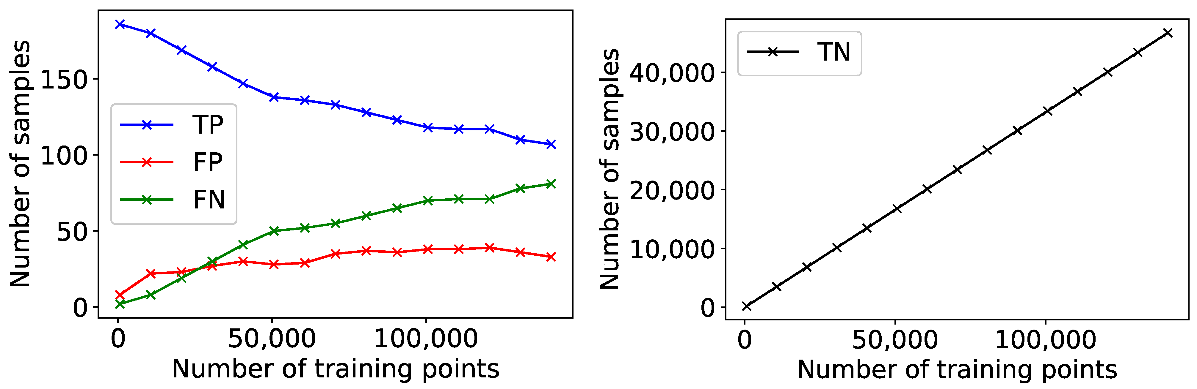
To further examine the performance of the model, a learning curve was obtained. This allows to determine the model performance as a function of the number of training points used, and is shown in Figure 3. The ground truth corresponding to the training points has been generated by manually selecting the points that according to human judgement corresponded to outliers. Each point in the curves represents the number of True Negatives (TN), True Positives (TP), False Negatives (FN), and False Positives (FP) obtained on a test data set whose size corresponds to 25% of the overall data set available, which is made up of some thousands of numerical simulations of DA for both the LHC and HL-LHC rings, when the model is trained on all anomalous points plus a certain increasing number of normal points. A TP is a ground-truth anomalous point, which was correctly predicted as being anomalous. The results show that when the training data set is approximately balanced between abnormal and normal points, the number of TP is quite high, while the FP and FN are low. However, as the data set skews towards an increasing majority of normal points, the model achieves a lower performance. This is understandable given the assumption of balance in the SVM algorithm.
Two UL approaches for detecting anomalies on an angle-by-angle basis have been considered, too. The first algorithm is the Density-Based Spatial Clustering of Applications with Noise (DBSCAN) [34]. DBSCAN is a density-based, non-parametric algorithm, which groups points based on local density of samples. The points that are not assigned to any cluster after applying the algorithm are automatically considered to be outliers. The second algorithm is the Local Outlier Factor (LOF) [35] method. LOF also uses the concept of local density, but directly computes an outlier score per point. Locality is provided by the K nearest neighbors, whose distance is used to estimate the density. By comparing the local density of an object to the local densities of its neighbors, it is possible to identify regions of similar density. Therefore, it is clear that points that have a substantially lower density than their neighbors are to be considered as outliers.
For the UL approach, 75% of the data set was used for training and 25% was used for validation. As a result of hyperparameter optimization through a grid search, the following is a list of the hyperparameters determined for each method:
  • DBSCAN: eps = 1 (the maximum distance between two samples for one to be considered as in the neighborhood of the other); min_samples = 3 (the number of samples, or total weight, in a neighborhood for a point to be considered as a core point, including the point itself);
  • LOF: n_neighbors = 58 (the number of neighbors used to measure the local deviation of density of a given sample with respect to the same neighbors); contamination = 0.001 (the expected fraction of outliers in the data set).
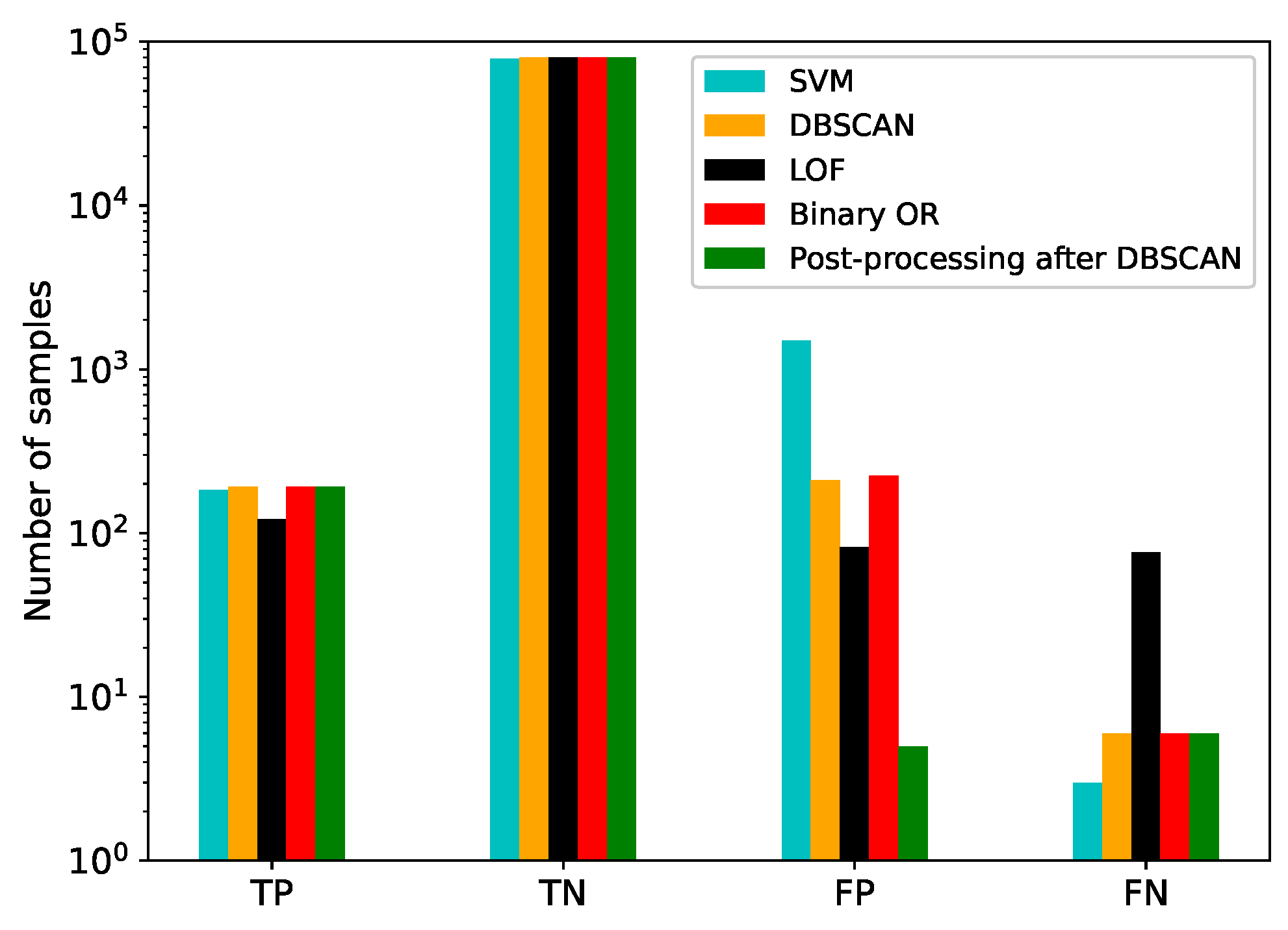
A comparison between the performance of the SVM, DBSCAN, and LOF algorithms is shown in Figure 4. The Python-based scikit-learn [36] implementation of these three algorithms was used. The labels determined by the DBSCAN and LOF algorithms were also combined through a binary OR operation to produce a fourth set of labels. A further fifth set of labels was created following an initial labelling by DBSCAN by removing false positives through a statistical method to determine whether this approach would add to the robustness of the original prediction. For a point, being originally flagged by DBSCAN as an outlier, to be considered as a true outlier, three additional criteria should be fulfilled: the distance from the mean should be at least 3 σ (where mean and standard deviation are only calculated over the normal points); the distance to the nearest normal point should be greater than 0.15 , in absolute units, and the distance to the nearest regular point should be greater than 34 % of the total spread of the regular points. This post-processing is performed iteratively, starting at the minimum (maximum) point and moving outwards (inwards), recalculating the statistical variables of the regular points at every step. The values of these thresholds are chosen empirically to ensure that false positives that are due to dense clusters are correctly filtered out.
The results show that the unsupervised learning methods perform better than SVM by an order of magnitude in terms of false positives; however they are worse in terms of false negatives, especially in the case of LOF. The method of post-processing following DBSCAN clearly contributes to reducing the number of false positives, while maintaining the TP and FN rates.
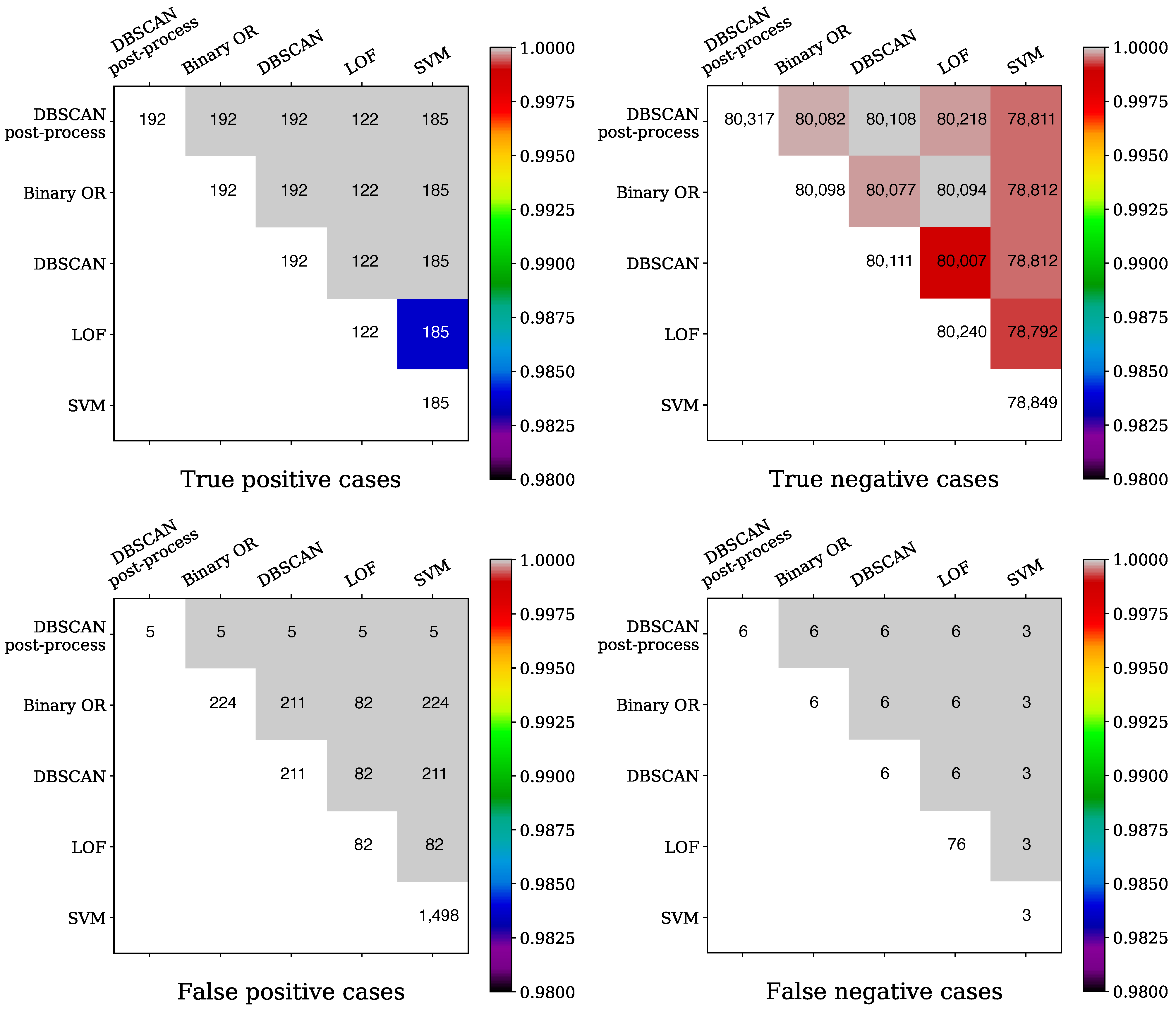
Additional detail on the impact of the post-processing is visible in Figure 5, in which the number of events for the various methods applied, and the size of the intersection of the events between pairs of methods, is shown for the four classes of TP, TN, FP, and FN cases.
Each heat map reports along the diagonal the number of events for each method of a given class, i.e., TP, TF, FP, and FN. In the upper triangular part of the matrix, the number of events in the intersection between the methods taken in pairs is shown; the color used is selected by normalizing the number of events in the intersection by the minimum of the events for the considered pair of methods. The level of TP cases is very similar for most of the methods, whereas differences are observed concerning the TN cases, and there the post-processing ensures that the higher score of TN cases is reached. As far as the FP and FN cases are concerned, it is clear that the post-processing provides the least number of events for FP cases, which is a very important feature. Similarly, FN cases are minimized by the post-processing, although the same number is obtained by the binary OR or plain DBSCAN. SVN scored excellently in FN, but was rather poor in the other three classes. All in all, the proposed post-processing of the DBSCAN clearly outperformed the other methods and provided a level of FP and FN cases that is perfectly adequate for our needs.

4.2. Digression: Accelerator Physics Considerations from Outlier Identification in DA Simulations

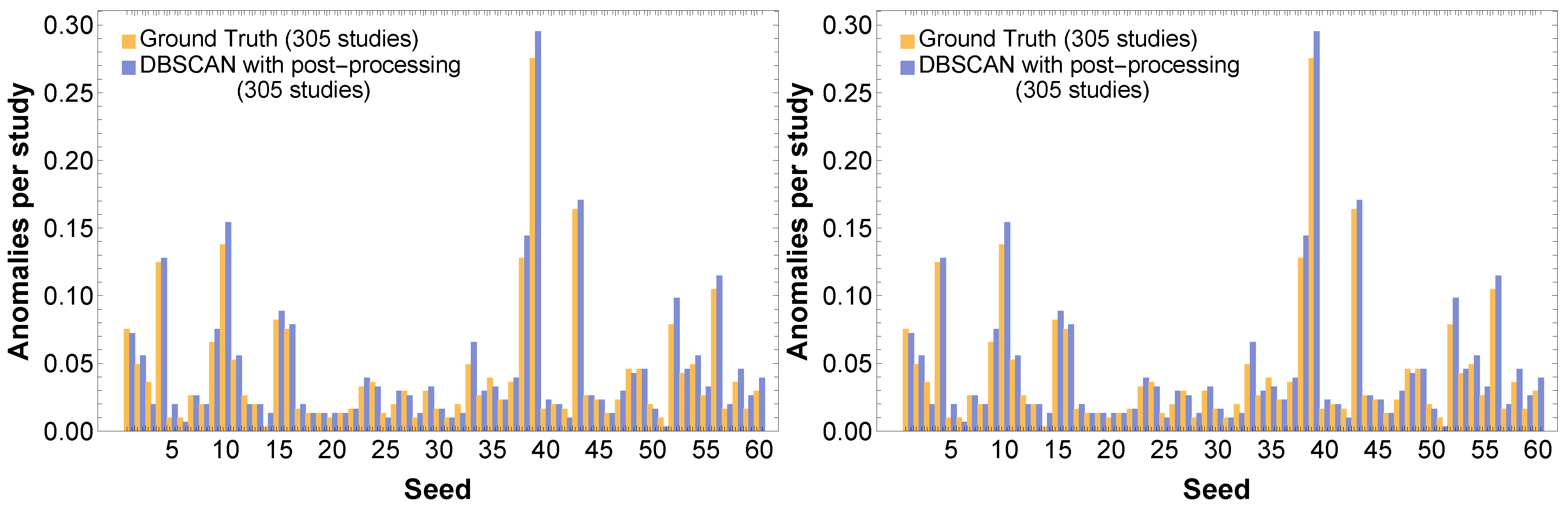
It is very useful to investigate the dependence of the number of outliers on the value of the angular variable and on the seed number. A comparison between the ground-truth and predicted anomalies (using post-processing following DBSCAN) is shown in Figure 6, where it can be seen that the anomaly profiles for both seeds and angles are similar between the ground-truth and the predictions. The peculiar profile of outliers as a function of seed is worth noting, featuring three clusters with a very large number of outliers. As far as the anomalies distribution as a function of angle is concerned, there is a tendency towards a larger number of outliers for angles close to 90 . It is worth stressing that there are outliers affecting the lower-amplitude part of the distribution or r i ( α j , N ) (outliers from below) or the higher-amplitude part (outliers from above). The analyses performed indicate that the number of outliers from below and those from above are essentially equal, totaling 2882 and 2847 cases, respectively.
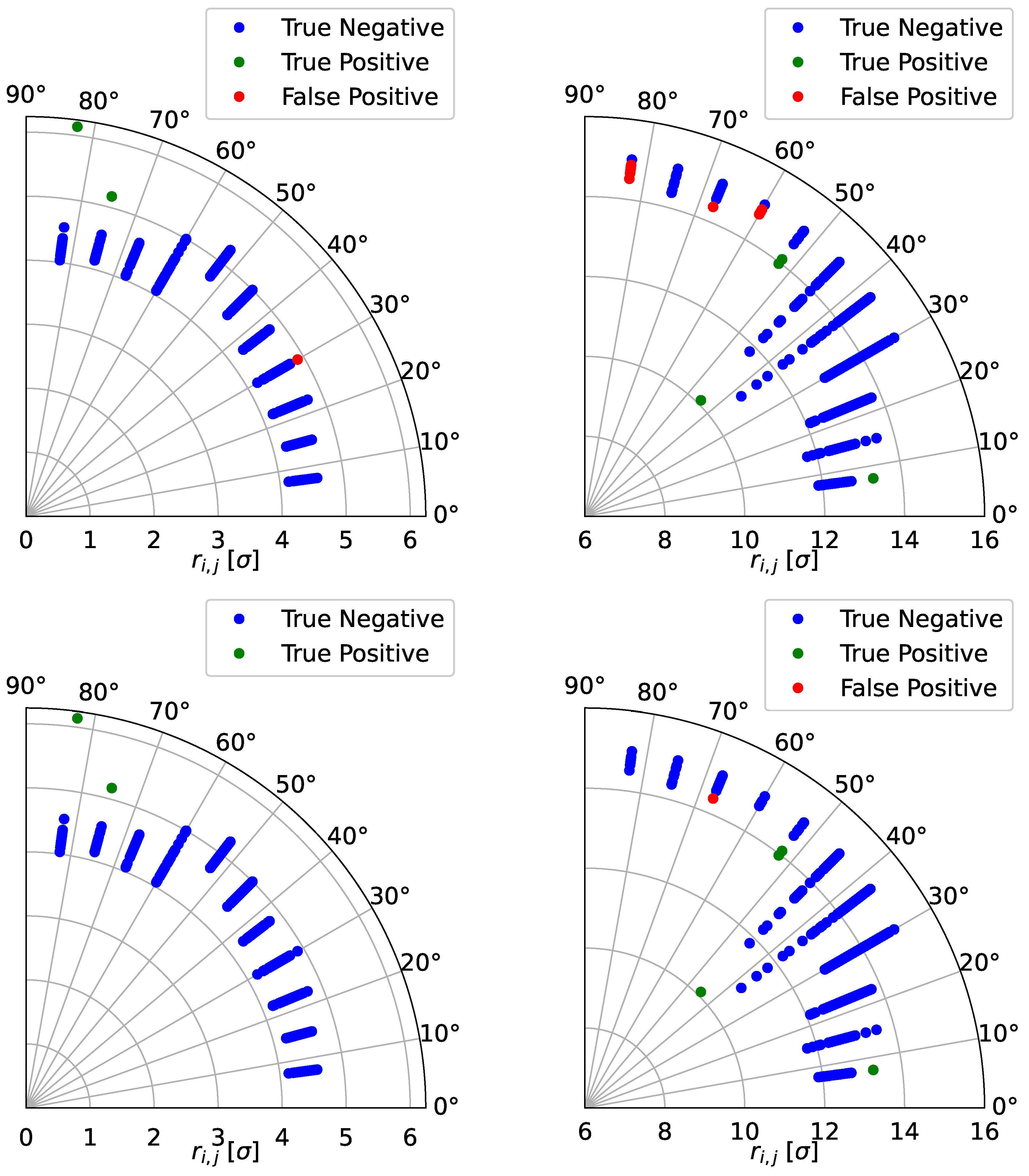
Two examples of the classification of outliers from normal points obtained by means of the post-processing following the DBSCAN method are shown in Figure 2.
It should be noted that the dynamics governing the DA can be very different as a function of the angle θ ; hence, even when the neighboring points are similar in amplitude, the spotted outlier might be a genuine one. Obviously, particular care needs to be taken in these cases before drawing any conclusions, and additional investigations might be advisable.
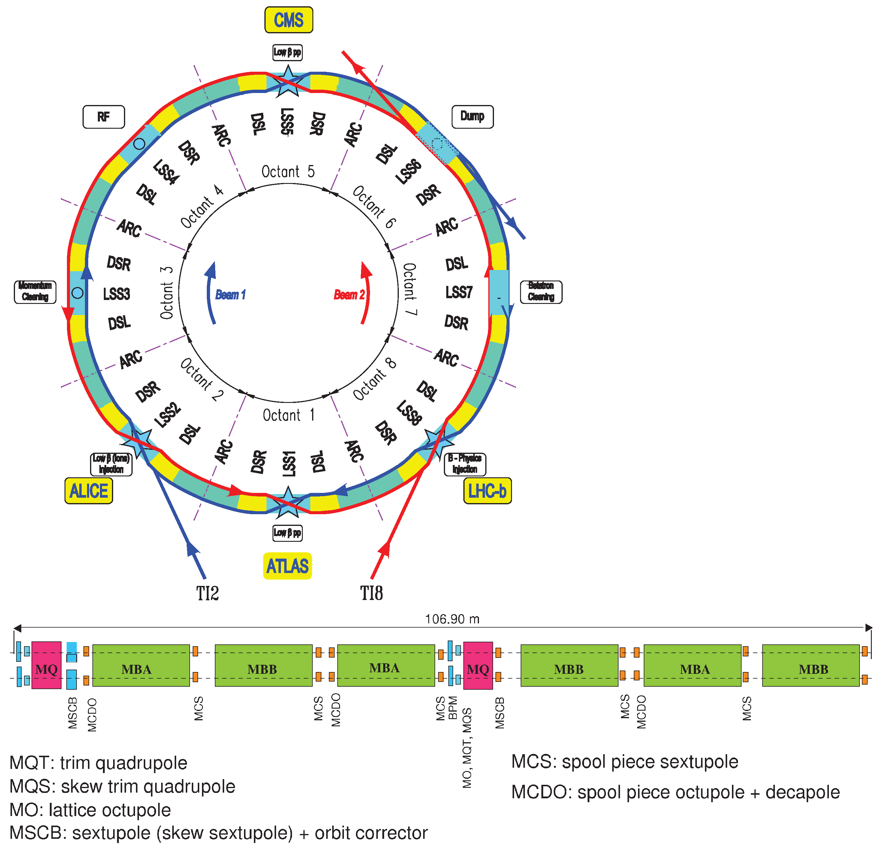
It is clear that the previous analysis provides useful insight into the underlying physics. Indeed, it is interesting to consider how the outliers are distributed over seeds and angles for the various configurations that make up the huge data set to which the analysis has been applied. The main cases covered by the numerical simulations can be categorized according to: accelerator (LHC or HL-LHC); beam energy (injection, 450 GeV, or top energy, 7 TeV); circulating beam (Beam 1, rotating clockwise, or Beam 2, rotating counter-clockwise); optical configuration of the accelerator (nominal [20] or ATS [37] for the LHC, and V1.0, V1.3, V1.4 for the HL-LHC); and the strength of the octupole magnets that are used to stabilize the beams against collective effects. In 
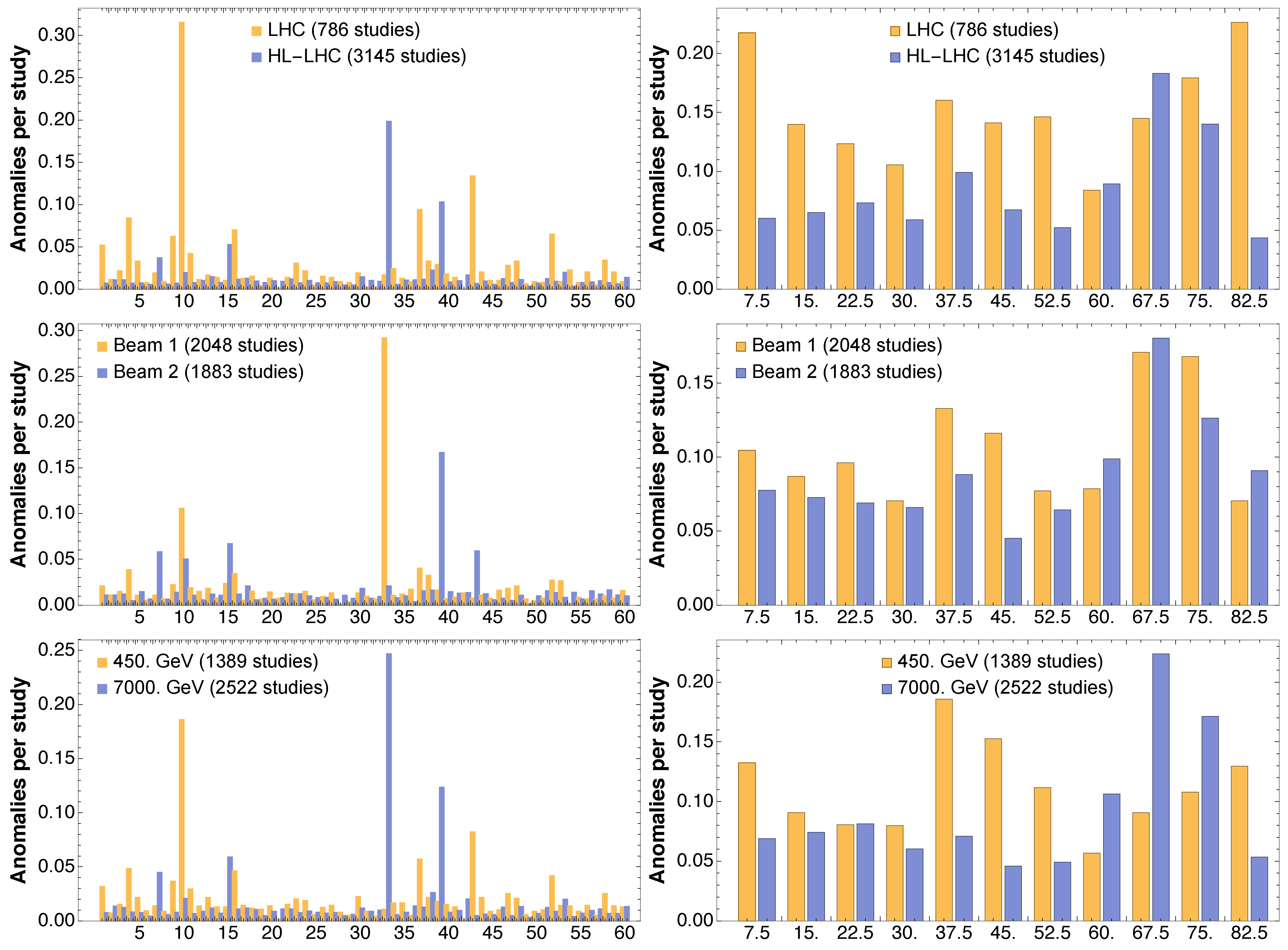
Figure 7, a collection of results of the obtained distributions of outliers vs. seed and angle are shown for several configurations probed with the numerical simulations.
The LHC and HL-LHC feature a different distribution of outliers, the first being affected by a number of outliers that are mildly dependent on the angles and special seed 10, whereas the latter features a mild increase of outliers towards a large angle and special seeds 33 and 39. While the two counter-rotating beams do not feature a meaningful differences in the distribution of outliers as a function of angle, with a sort of peak around 70 degrees, we can pinpoint the high number of anomalies for seed 33 to Beam 1 and those for seed 39 to Beam 2. On the other hand, the situation in terms of outliers when considering the injection or the collision energies is a bit different, inasmuch that at collision energy the distribution of anomalies is skewed towards larger angles. Note also that different seeds present anomalies depending on the value of the beam energy. Here it is worth mentioning that the overall data set is skewed towards HL-LHC cases, which, in turn, feature mainly collision-energy cases. On the other hand, the LHC cases refer mainly to the injection energy case. This explains some of the similarities in the behavior of anomalies as a function of the ring considered and on the beam energy.
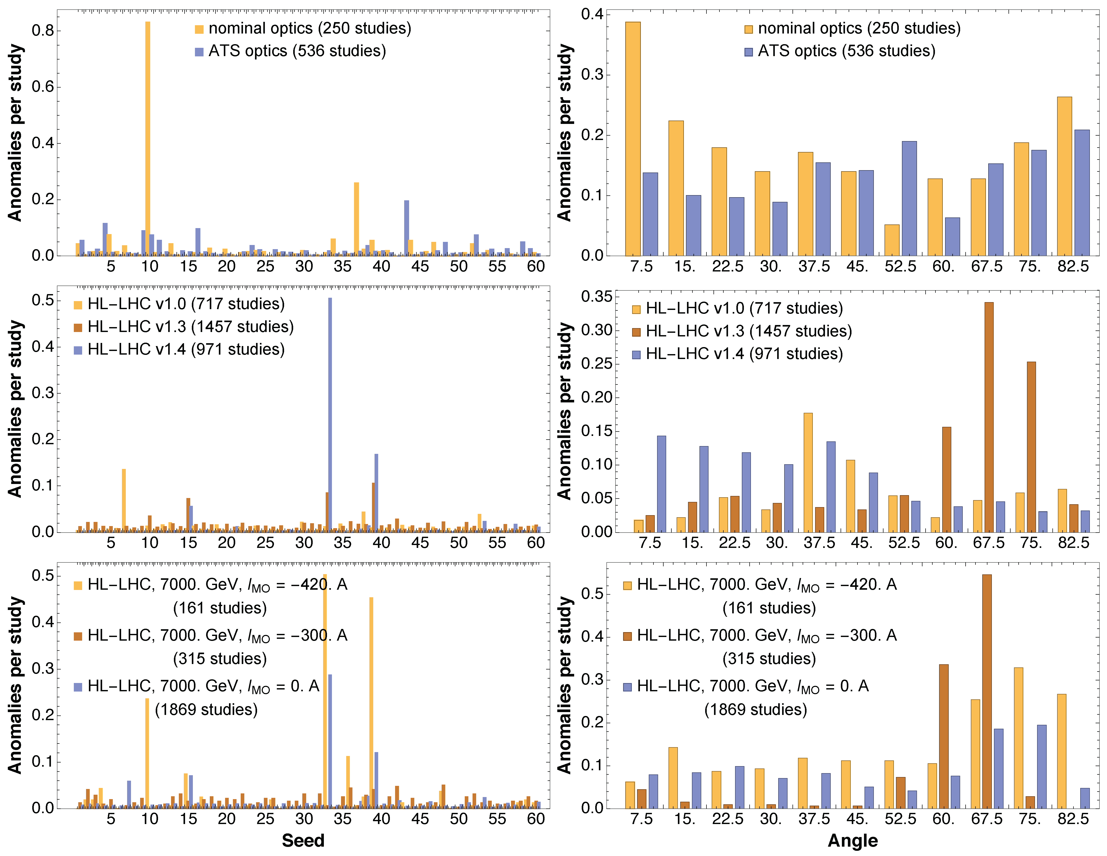
In terms of optical configuration used for the LHC, the nominal one features a special seed 10, and outliers towards low angle values. On the other hand, ATS shows essentially no anomalous seeds and a very small number of anomalies as a function of angle.
The situation concerning different ring layouts and optics versions that are being studied for the HL-LHC shows an interesting evolution in terms of the appearance of anomalous seeds as of version V1.3. This is also combined with a change in terms of distribution of outliers as a function of angle. Indeed, while version V1.0 features outliers mainly in the middle range of angles, version V1.3 is characterized by outliers towards the high range of angles. The situation then changes with version V1.4, where an increase of outliers is observed towards the low range of angles. Interestingly enough, the presence of strong octupoles used to stabilize the beams has an adverse effect in terms of anomalous seeds and outliers vs. angle. In fact, a clear increase of anomalies can be observed with increasing, in absolute value, current in the Landau octupoles. This feature appears in conjunction with an increased number of anomalies for large values of angles.
It is worth stressing that the observed features of the distribution of outliers for LHC and HL-LHC will be carefully considered to shed some light on the underlying beam dynamics phenomena that are responsible for their generation.

4.3. Fitting the DA as a Function of Number of Turns

Another domain where ML techniques have been applied, with the hope that they can bring improvements, is the modeling of the DA as a function of the number of turns. In Section 3, the concept of DA has been introduced and briefly discussed; it can be estimated by means of numerical simulations that are performed for a given number of turns N max . The main observation is that the DA tends to shrink with time, which is logical as by increasing the number of turns even initial conditions with a low-amplitude might turn increase it, either slowly or more abruptly, due to the presence of nonlinear effects. The second fundamental observation is that the variation of the DA with the turn number can be described with rather simple functional forms (see, e.g., Equation (12)) that feature a very limited number of free parameters.
The approach pursued by our research consists of fitting one of the scaling laws to the numerical data and performing extrapolation over the number of turns N so as to make predictions of the DA value for N N max that would be inaccessible to numerical simulations, because of the excessive computing time needed. We stress once more that the concept of DA at turn number N can be linked with that of beam intensity at the same time N [28]. This means that the knowledge of the evolution of the DA, i.e., a rather abstract quantity, can be directly linked to the evolution of the beam intensity in a circular particle accelerator, which is a fundamental physical observable. This approach has been already successfully applied in experimental studies [38] and intense efforts are devoted to refine and promote the proposed strategy.
A detailed analysis has been presented in Reference [24], where the extrapolation error has been considered as a key figure of merit to qualify the models describing the DA evolution. The key improvement that can be brought to the DA modeling by ML is to improve the extrapolation error. However, it is generally believed that ML has serious limitations in providing efficient answers to extrapolation problems. Therefore, the devised approach is based on a different strategy. It consists in training a Gaussian Process (GP) (see, e.g., [
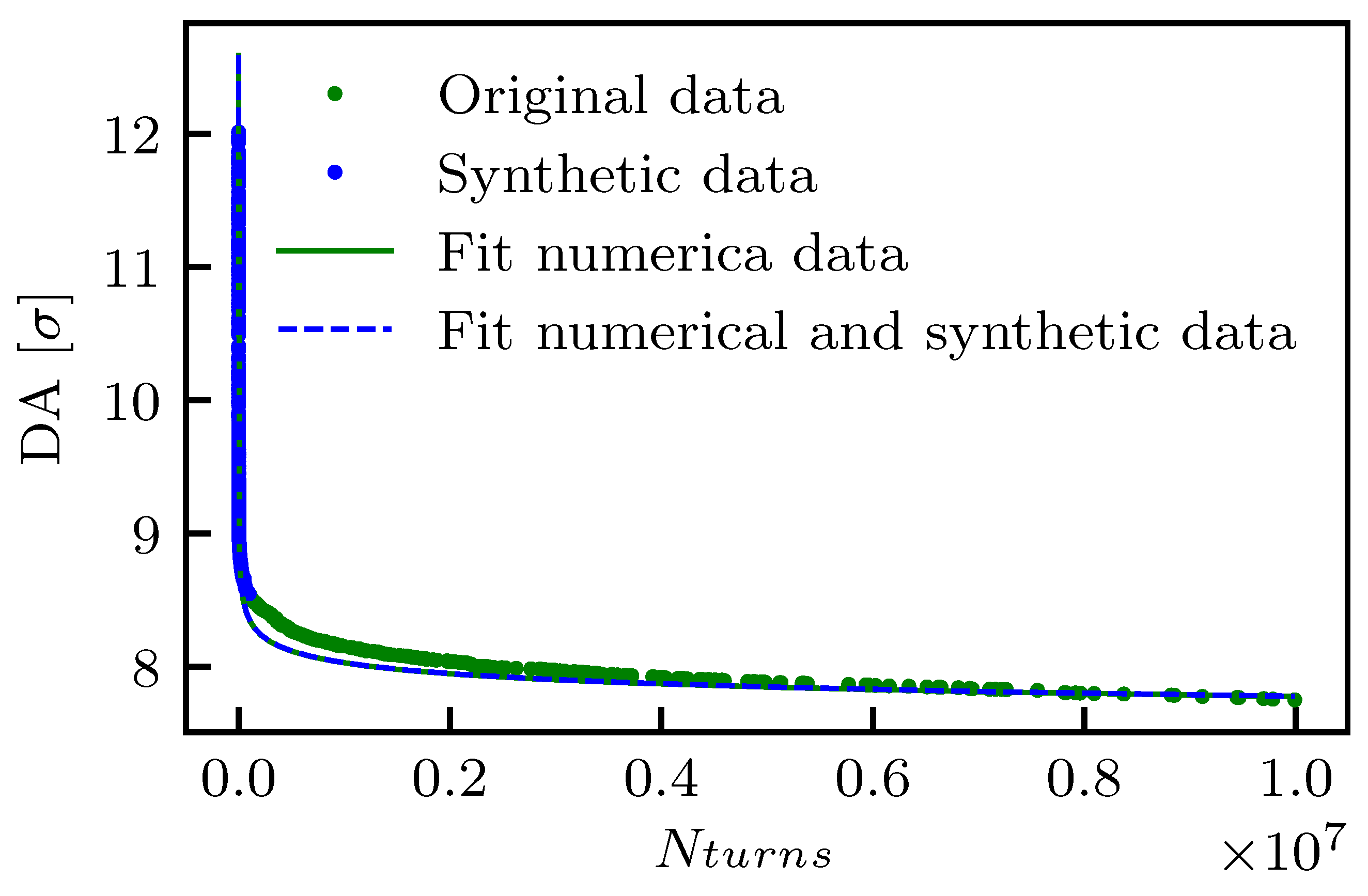
39]) on the available DA evolution data to generate synthetic, though realistic, points that are used to increase the overall density of points, which are then used to create the model. In this way, ML is used to provide interpolated points, which is a task that can be dealt with very efficiently. This considerably improves the extrapolation capabilities of the fitted model as the results of our studies indicate clearly. In Figure 8 an example of the proposed fit based on the DA model (14b) with three parameters and with the addition of synthetic points determined by means of a GP is shown for reference. In this specific case, the original fit approach and that based on the GP provide very similar results.
Out of the large pool of several thousands of DA simulations performed for LHC and HL-LHC, a single study with N max 5 × 10 5 has been selected at random and 50 values of turns N i have been distributed uniformly between N = 1 × 10 4 and N = 1 × 10 5 . The corresponding values DA i = DA ( N i ) have been generated by means of the GP and then a fit of the DA data (numerical plus synthetic points) was performed using model (14b), and this procedure was repeated 5 × 10 5 times, each time computing the Mean Square Error (MSE) ϵ . Note that, indeed, two variants have been tested, namely using three fit parameters ( ρ , μ , κ ), or two ( ρ , κ ), in which μ was expressed as a function of ρ , κ according to Equation (15). It is worth mentioning that whenever the GP is used, the MSE of the fitted model is computed disregarding the synthetic points, i.e., using only the points obtained from the DA simulations. In this way, we can perform a fair comparison between the MSE for the original fit and that performed with the help of GP.
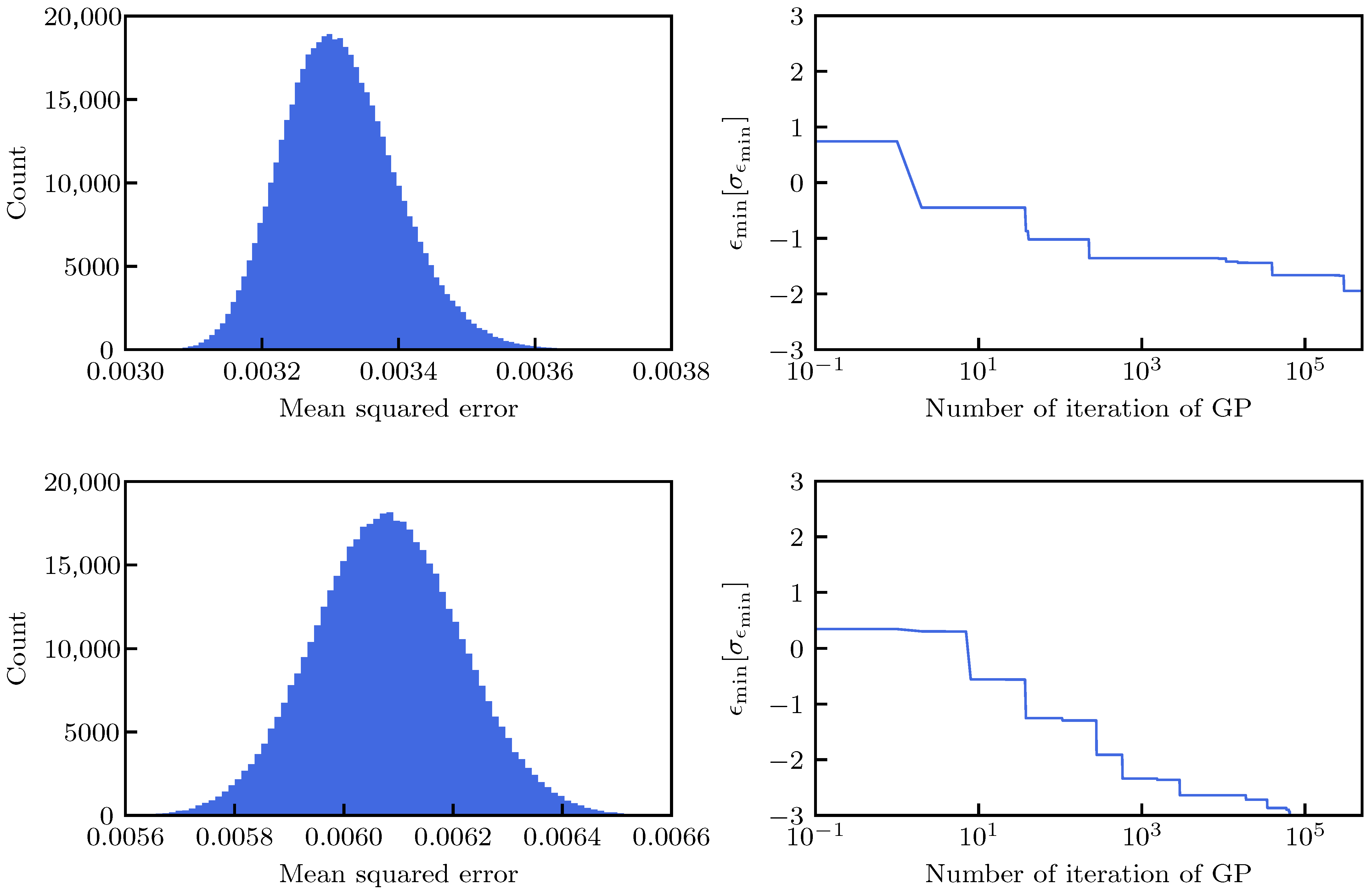
The resulting distribution of the MSE is shown in Figure 9 (left) for the case of the three-(top) and two-parameter (bottom) fit.
The shape of the MSE distribution for the three-parameter fit is located closer to zero and its width is smaller than the corresponding distribution for the two-parameter fit. The former is logical as a model with more parameters that has more possibility to tune and typically will have a better MSE, while the latter implies that the iterative application of the GP can provide a larger improvement in the MSE in the case of the two-parameter fit. It is worth noting that while the MSE distribution for the three-parameter fit is right-skewed, that for the two-parameter fit is left-skewed.
In the right-hand plots of Figure 9, the behavior of the following quantity is shown:
ϵ min , i = min 0 < j < i ϵ j GP ϵ GP σ ϵ GP 0 i 5 × 10 5 ,
which is the minimum, over the iterations of the GP process, expressed as its normalized distance to the average MSE. The average MSE, ϵ GP , and its variance, σ ϵ GP , used to express ϵ min , i , are calculated over the full set of 5 × 10 5 iterations and are reported in Table 1. The initial value ϵ min , 0 is not particularly meaningful, whereas the variation can be used as an estimate of the rate of improvement of the MSE with the number of iterations of the GP. Another interesting variable to investigate is the relative gain, w.r.t the original fit, of the minimum MSE after i iterations:
δ ϵ min , i = ϵ original ϵ GP ϵ min , i σ ϵ GP ϵ original 0 i 5 × 10 5 ,
which is also reported in Table 1. For both fit types, i.e., with two or three parameters, a number of iterations of about 10 3 would seem to induce a sizeable reduction of the MSE. However, looking at δ ϵ min , it becomes clear that going from 10 2 to 10 3 iterations only induces an extra gain of around 1% (even considering that ϵ min , i doubles in case of the two-parameter fit). This can be explained by observing that ϵ GP is already multiple σ ϵ GP units away from the MSE of the original fit. Knowing this, and taking into consideration that in the case of analyses of a large set of DA simulations a trade-off between CPU time and final value of MSE needs to be found, we consider a value of around 10 2 GP iterations to be sufficient.
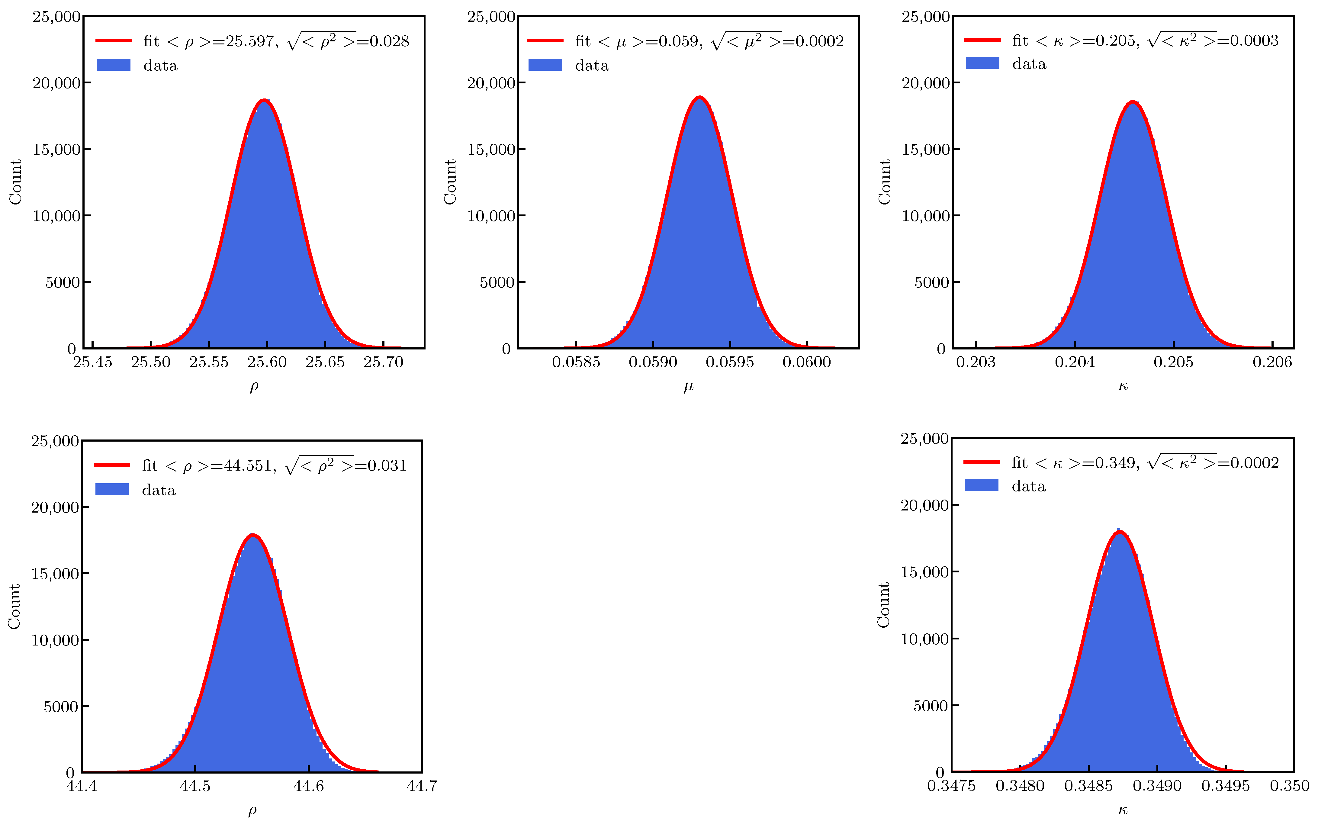
The distribution of the parameters describing the DA evolution with time is shown in Figure 10 for the three- (top) and two-parameter (bottom) cases.
Gaussian fits to the model parameters are provided for reference, and while these fits are in excellent agreement with the numerical data for the three-parameter case, slight asymmetries of the parameter distributions are visible for the two-parameter case. Although the mean values of the common fit parameters, i.e., ρ and κ , are different for the two types of fits, the absolute values of their RMS values are very similar.
As mentioned earlier, the main use of the DA models is to provide an accurate tool to extrapolate DA beyond a number of turns N that is currently feasible with the CPU power available to our numerical simulations. Therefore, it is essential to probe the accuracy of the prediction of the fitted model. To this aim, a set of six DA simulations performed using a LHC lattice at injection energy and with a maximum number of turns of 10 7 (note that the standard value of turns is 10 5 , when beam–beam effects are neglected but magnetic fields errors are included, or 10 6 when beam–beam effect are included and the magnetic field errors are neglected). The large number of turns simulated, which accounts for only 889 s of beam revolutions in the ring with respect to several hours of a typical fill, allow the accuracy of the prediction power of the DA model to be probed accurately. This is done by setting the value of the maximum number of turns N max of the numerical data that are used to fit the DA model. Such a model is then used to extrapolate the DA up to 10 7 turns, and the MSE is evaluated over the full set of numerical data up to 10 7 turns. All of this is repeated by varying N max . The same procedure is applied when the GP is used to improve the quality of the fitted model. In this case, 75 additional points are uniformly distributed between 10 4 N N max when N max = 5 × 10 5 , and the number of synthetic points is linearly increased to reach 750 when N max = 5 × 10 6 . Once more, we recall that the synthetic points are not considered when computing the MSE for the GP-based fit, which ensures a fair comparison between the MSE of the original and GP-based fits. Also in this application of the GP-based fit, the GP part is repeated 200 times and the minimum MSE error over the 200 iterations is used. Lastly, all of these protocols are repeated for the three- and two-parameter fit of the DA model.
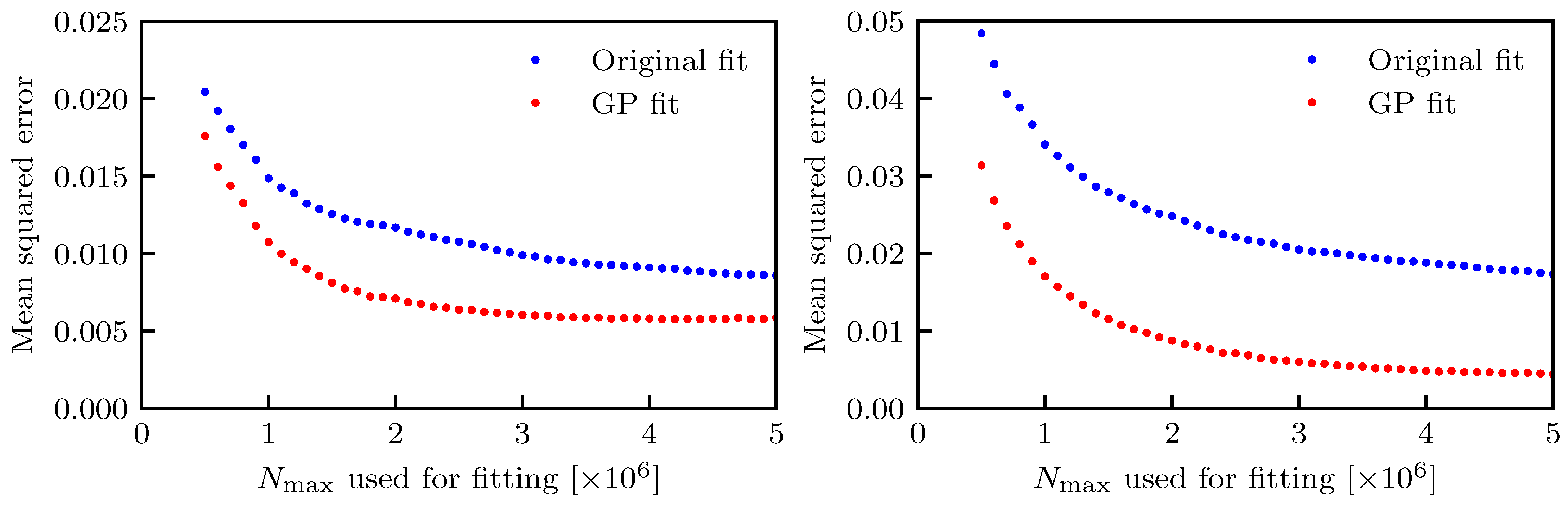
The results are shown in Figure 11, where the case of three- and two-parameters fit are shown in the left and right plots, respectively.
The metrics used to quantify the performance in terms of extrapolation could have been the determination of the difference between the DA value at 10 7 turns computed from numerical simulations and that obtained from the fitted DA models. However, it has been chosen to apply the MSE computed over the entire set of points from the tracking simulations. Indeed, this approach is much more robust, as it estimates the fit performance by using the information carried by the full set of points, rather than a single point.
The key point is that the MSE for the GP-based fit is always better than that of the corresponding original fit, which clearly indicates the success of the proposed approach. Some sort of saturation in the decrease of the MSE is visible for N max 2 5 × 10 6 for the three-parameter fit, which indicates that the numerical simulations carried out up until any of the turn numbers in that interval allow a reliable extrapolation up to 10 7 turns. No qualitative difference was observed for the two types of fits: as expected, the initial MSE value was larger for the case of two- with respect to the case of three-parameter fit. However, the MSE decreased steadily as a function of N max , and the MSE for the GP-based fit reached a final comparable value no matter the value of the number of free fit parameters. In fact, as previously mentioned, the GP was more efficient in improving the two- than the three-parameter fit, as the MSE for N max = 5 × 10 6 was reduced from 1.7 × 10 2 (original fit) to 4.5 × 10 3 (GP fit) for the two-parameter case (a reduction of 74%), whereas a reduction from 8.5 × 10 3 (original fit) to 5.8 × 10 3 (GP fit) for the three-parameter case (a reduction of 32%) was observed.
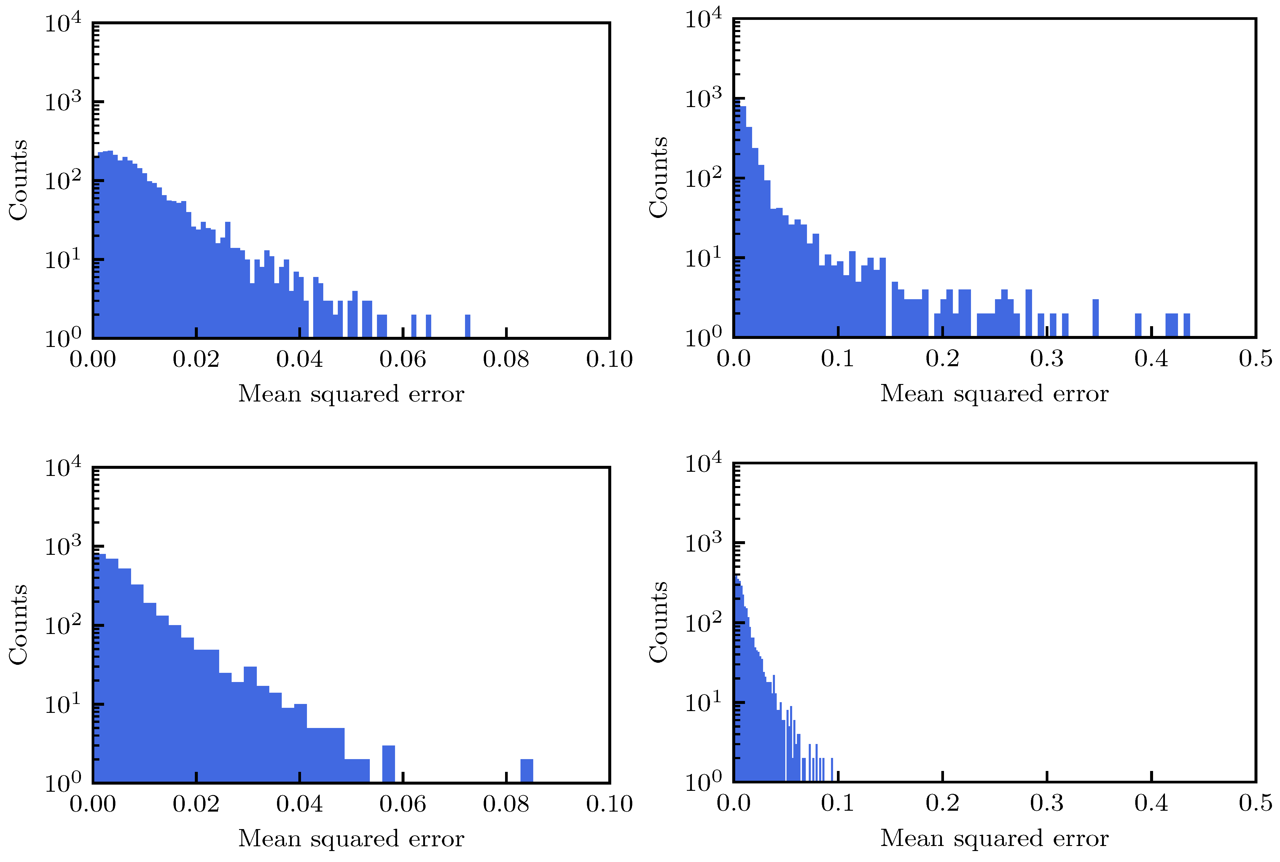
As a last investigation, the behavior of the proposed method based on ML was probed on a large set of DA simulations, corresponding to 3090 cases of the LHC lattice at injection energy for various configurations of the strength of the octupoles and values of the linear chromaticity. The fits were performed using N max = 1 × 10 5 and then extrapolating the fitted function up until 10 6 turns and evaluating the MSE. Whenever the GP was used, 50 iterations were applied (this number is slightly sub-optimal, but it was chosen as a trade-off between the improvement achieved by the iterations of the GP and the CPU time required by this study (the generation of the plots shown in Figure 12 took several hours) and in addition to the MSE for each fit type, the difference of MSE values, i.e., Δ MSE = MSE originalfit MSE GPfit was considered to provide an easy comparison between the two approaches. As in the previous studies, both three- and two-parameter DA models were used and the summary plots are shown in
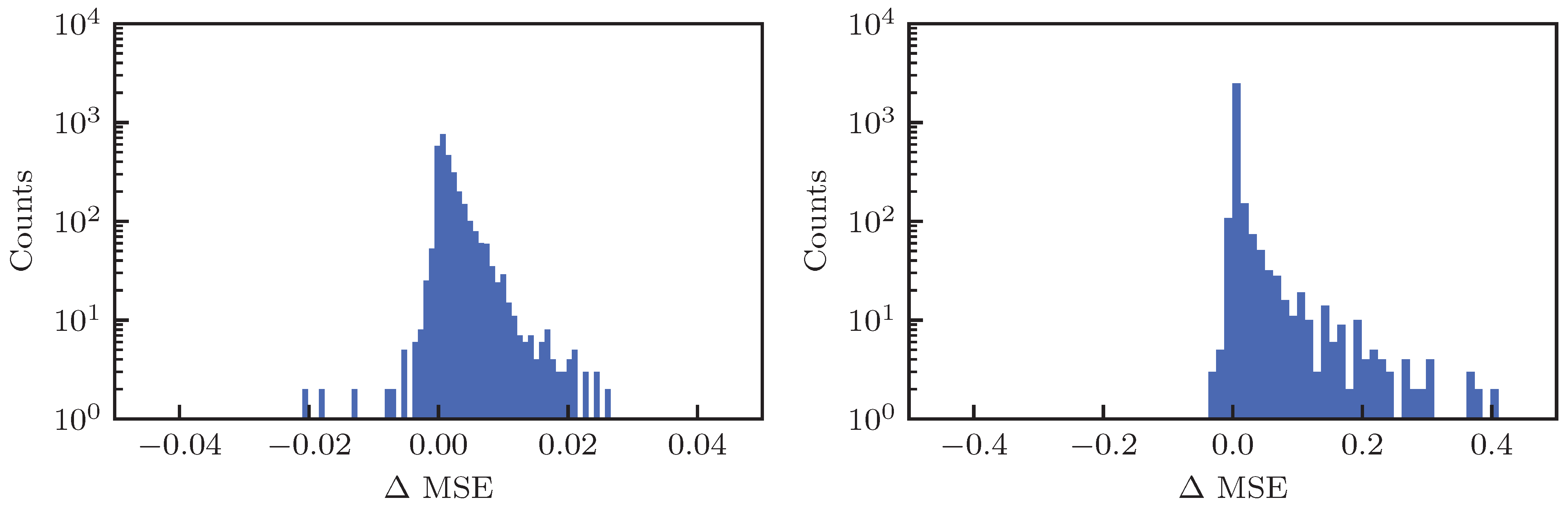
 Figure 12.
The results for the three-parameter fit are reported in the left column, whereas those for the two-parameter fit are reported in the right one. In the first and second rows the distribution of the MSE for the original fit and for that with GP are shown, respectively; whereas in the third row the distribution of Δ MSE is reported. Globally, the MSE for the three-parameter fit is smaller than that of the two-parameter fit, and the fit with GP has a better performance in terms of MSE than the original one. This is clearly visible for the two-parameter fit, but is also the case for the three-parameter variant. This can be appreciated in Table 2, where some statistical parameters of the distributions are reported: the improvement in terms of MSE distribution brought by the GP is clear, and very much visible, in particular for the two-parameter fit.
As far as the distribution of Δ MSE is concerned, its positive part shows how many DA simulations have been improved by means of the GP fit, wheres the negative part shows the case in which the GP fit has worsened the DA model. Although there are some DA simulations for which the GP fit produced a slight worsening, it is worth mentioning that this set corresponds to 13% and 8% for the three- and two-parameter fits, respectively. It is exactly for this reason that one should not use a single iteration of the GP process as a means to improve the fit. As mentioned before, a value of around 10 2 iterations seems appropriate to improve the fitting quality overall.

5. Conclusions

In this paper, results of some recent applications of ML techniques to the analysis of nonlinear beam dynamics in the LHC and its luminosity upgrade have been presented and discussed in detail. Two topics have been addressed, namely the identification of outliers in dynamic aperture simulations and the improvement of the fit of DA models to numerical simulation data.
In both cases, the ML techniques proved to be an efficient approach to improve the current status of our tools. Outliers can be effectively identified and rejected using techniques to analyze the distribution in phase space of points obtained via numerical simulations. Analysis of dynamic aperture evolution with number of turns also showed considerable improvement by using a Gaussian process to add synthetic data to numerical simulations, improving the reliability of fits of recently developed models for DA evolution and aiding in the extrapolation of such numerical simulations to timescales relevant to collider operation.
All in all, the very encouraging results presented in this paper confirm the possibility of creating a fruitful exchange between the domain of ML and nonlinear beam dynamics.

Author Contributions

Software, C.E.M., G.V. and F.F.V.d.V.; formal analysis, M.G., G.V. and F.F.V.d.V.; investigation, M.G., G.V. and F.F.V.d.V.; data curation, E.M.; writing—original draft preparation, M.G.; writing—review and editing, M.G. All authors have read and agreed to the published version of the manuscript.

Funding

This research was partially funded by the HL-LHC Project.

Conflicts of Interest

The authors declare no conflict of interest.

Abbreviations

The following abbreviations are used in this manuscript:
ATSAchromatic Telescopic Squeezing
DADynamic Aperture
DBSCANDensity-Based Spatial Clustering of Applications with Noise
DLDeep Learning
GPGaussian Process
HL-LHCHigh-Luminosity LHC
LEPLarge Electron Positron collider
LHCLarge Hadron Collider
LOFLocal Outlier Factor
MLMachine Learning
MSEMean Square Error
NANot applicable
RBFRadial Basis Function
RLReinforcement Learning
RMSRoot Mean Square
SLSupervised Learning
SVMSupport Vector Machines
ULUnsupervised Learning

References

  1. Mitchell, T.M. Machine Learning; McGraw-Hill: New York, NY, USA, 1997. [Google Scholar]
  2. Bonaccorso, G. Hands-On Unsupervised Learning with Python: Implement Machine Learning and Deep Learning Models Using Scikit-Learn, TensorFlow, and More; Packt Publishing: Birmingham, UK, 2019. [Google Scholar]
  3. Hussein, S.; Kandel, P.; Bolan, C.W.; Wallace, M.B.; Bagci, U. Lung and Pancreatic Tumor Characterization in the Deep Learning Era: Novel Supervised and Unsupervised Learning Approaches. IEEE Trans. Med Imaging 2019, 38, 1777–1787. [Google Scholar] [CrossRef] [PubMed] [Green Version]
  4. Bonetta, R.; Valentino, G. Machine learning techniques for protein function prediction. Proteins Struct. Funct. Bioinform. 2020, 88, 397–413. [Google Scholar] [CrossRef] [PubMed]
  5. Lien Minh, D.; Sadeghi-Niaraki, A.; Huy, H.D.; Min, K.; Moon, H. Deep Learning Approach for Short-Term Stock Trends Prediction Based on Two-Stream Gated Recurrent Unit Network. IEEE Access 2018, 6, 55392–55404. [Google Scholar] [CrossRef]
  6. Dal Pozzolo, A.; Boracchi, G.; Caelen, O.; Alippi, C.; Bontempi, G. Credit Card Fraud Detection: A Realistic Modeling and a Novel Learning Strategy. IEEE Trans. Neural Netw. Learn. Syst. 2018, 29, 3784–3797. [Google Scholar] [CrossRef] [PubMed]
  7. Chalup, S.K.; Murch, C.L.; Quinlan, M.J. Machine Learning With AIBO Robots in the Four-Legged League of RoboCup. IEEE Trans. Syst. Man Cybern. Part C (Appl. Rev.) 2007, 37, 297–310. [Google Scholar] [CrossRef]
  8. Su, J.; Wu, J.; Cheng, P.; Chen, J. Autonomous Vehicle Control Through the Dynamics and Controller Learning. IEEE Trans. Veh. Technol. 2018, 67, 5650–5657. [Google Scholar] [CrossRef]
  9. LeCun, Y.; Bengio, Y.; Hinton, G. Deep learning. Nature 2015, 521, 436–444. [Google Scholar] [CrossRef]
  10. Radovic, A.; Williams, M.; Rousseau, D.; Kagan, M.; Bonacorsi, D.; Himmel, A.; Aurisano, A.; Terao, K.; Wongjirad, T. Machine learning at the energy and intensity frontiers of particle physics. Nature 2018, 560, 41–48. [Google Scholar] [CrossRef]
  11. Bozoki, E.; Friedman, A. Neural networks and orbit control in accelerators. In Proceedings of the 4th European Particle Accelerator Conference (EPAC’94), London, UK, 27 June–1 July 1994; pp. 1589–1592. [Google Scholar]
  12. Meier, E.; Tan, Y.E.; LeBlanc, G. Orbit Correction Studies using Neural Networks. In Proceedings of the 3rd International Particle Accelerator Conference (IPAC’12), New Orleans, LA, USA, 20–25 May 2012; pp. 2837–2839. [Google Scholar]
  13. Li, Y.; Cheng, W.; Yu, L.H.; Rainer, R. Genetic algorithm enhanced by machine learning in dynamic aperture optimization. Phys. Rev. Accel. Beams 2018, 21, 054601. [Google Scholar] [CrossRef] [Green Version]
  14. Emma, C.; Edelen, A.; Hogan, M.J.; O’Shea, B.; White, G.; Yakimenko, V. Machine learning-based longitudinal phase space prediction of particle accelerators. Phys. Rev. Accel. Beams 2018, 21, 112802. [Google Scholar] [CrossRef] [Green Version]
  15. Vilsmeier, D.; Sapinski, M.; Singh, R. Space-charge distortion of transverse profiles measured by electron-based ionization profile monitors and correction methods. Phys. Rev. Accel. Beams 2019, 22, 052801. [Google Scholar] [CrossRef] [Green Version]
  16. Wan, J.; Chu, P.; Jiao, Y.; Li, Y. Improvement of machine learning enhanced genetic algorithm for nonlinear beam dynamics optimization. Nucl. Instrum. Methods Phys. Res. A 2019, 946, 162683. [Google Scholar] [CrossRef]
  17. Leemann, S.C.; Liu, S.; Hexemer, A.; Marcus, M.A.; Melton, C.N.; Nishimura, H.; Sun, C. Demonstration of Machine Learning-Based Model-Independent Stabilization of Source Properties in Synchrotron Light Sources. Phys. Rev. Lett. 2019, 123, 194801. [Google Scholar] [CrossRef] [PubMed] [Green Version]
  18. Xu, X.; Zhou, Y.; Leng, Y. Machine learning based image processing technology application in bunch longitudinal phase information extraction. Phys. Rev. Accel. Beams 2020, 23, 032805. [Google Scholar] [CrossRef] [Green Version]
  19. Edelen, A.; Mayes, C.; Bowring, D.; Ratner, D.; Adelmann, A.; Ischebeck, R.; Snuverink, J.; Agapov, I.; Kammering, R.; Edelen, J.; et al. Opportunities in Machine Learning for Particle Accelerators. arXiv 2018, arXiv:1811.03172. [Google Scholar]
  20. Brüning, O.S.; Collier, P.; Lebrun, P.; Myers, S.; Ostojic, R.; Poole, J.; Proudlock, P. LHC Design Report; CERN Yellow Reports: Monographs; CERN: Geneva, Switzerland, 2004. [Google Scholar] [CrossRef]
  21. Arpaia, P.; Azzopardi, G.; Blanc, F.; Bregliozzi, G.; Buffat, X.; Coyle, L.; Fol, E.; Giordano, F.; Giovannozzi, M.; Pieloni, T.; et al. Machine learning for beam dynamics studies at the CERN Large Hadron Collider. Nucl. Instrum. Methods Phys. Res. A 2021, 985, 164652. [Google Scholar] [CrossRef]
  22. Giovannozzi, M.; McIntosh, E. Development of parallel codes for the study of nonlinear beam dynamics. Int. J. Mod. Phys. C 1996, 8, 155–170. [Google Scholar] [CrossRef] [Green Version]
  23. Barranco, J.; Cai, Y.; Cameron, D.; Crouch, M.; De Maria, R.; Field, L.; Giovannozzi, M.; Hermes, P.; Høimyr, N.; Kaltchev, D.; et al. LHC@Home: A BOINC-based volunteer computing infrastructure for physics studies at CERN. LHC@Home: A BOINC-based volunteer computing infrastructure for physics studies at CERN. Open Eng. 2017, 7, 378–392. [Google Scholar] [CrossRef]
  24. Bazzani, A.; Giovannozzi, M.; Maclean, E.H.; Montanari, C.E.; Van der Veken, F.F.; Van Goethem, W. Advances on the modeling of the time evolution of dynamic aperture of hadron circular accelerators. Phys. Rev. Accel. Beams 2019, 22, 104003. [Google Scholar] [CrossRef] [Green Version]
  25. Apollinari, G.; Béjar Alonso, I.; Brüning, O.; Fessia, P.; Lamont, M.; Rossi, L.; Tavian, L. High-Luminosity Large Hadron Collider (HL-LHC): Technical Design Report V. 0.1; CERN Yellow Reports: Monographs; CERN: Geneva, Switzerland, 2017. [Google Scholar] [CrossRef]
  26. Bestmann, P.; Bottura, L.; Catalan-Lasheras, N.; Fartoukh, S.; Gilardoni, S.; Giovannozzi, M.; Jeanneret, J.; Karppinen, M.; Lombardi, A.; Mess, K.; et al. Magnet Acceptance and Allocation at the LHC Magnet Evaluation Board. In Proceedings of the 2007 IEEE Particle Accelerator Conference (PAC), Albuquerque, NM, USA, 25–29 June 2007; p. 4. [Google Scholar] [CrossRef] [Green Version]
  27. Todesco, E.; Giovannozzi, M. Dynamic aperture estimates and phase-space distortions in nonlinear betatron motion. Phys. Rev. E 1996, 53, 4067–4076. [Google Scholar] [CrossRef] [Green Version]
  28. Giovannozzi, M. A proposed scaling law for intensity evolution in hadron storage rings based on dynamic aperture variation with time. Phys. Rev. ST Accel. Beams 2012, 15, 024001. [Google Scholar] [CrossRef]
  29. Giovannozzi, M.; Van der Veken, F.F. Description of the luminosity evolution for the CERN LHC including dynamic aperture effects. Part I: The model. Nucl. Instrum. Methods Phys. Res. A 2018, 905, 171–179, Erratum in 2019, 927, 471. [Google Scholar] [CrossRef]
  30. Giovannozzi, M.; Van der Veken, F.F. Description of the luminosity evolution for the CERN LHC including dynamic aperture effects. Part II: Application to Run 1 data. Nucl. Instrum. Methods Phys. Res. A 2018, 908, 1–9. [Google Scholar] [CrossRef]
  31. Nekhoroshev, N. An exponential estimate of the time of stability of nearly-integrable Hamiltonian systems. Russ. Math. Surv. 1977, 32, 1. [Google Scholar] [CrossRef]
  32. Boser, B.E.; Guyon, I.M.; Vapnik, V.N. A Training Algorithm for Optimal Margin Classifiers. In Proceedings of the Fifth Annual Workshop on Computational Learning Theory, COLT’92, Pittsburgh, PA, USA, 27–29 July 1992; Association for Computing Machinery: New York, NY, USA, 1992; pp. 144–152. [Google Scholar] [CrossRef]
  33. Vert, J.; Tsuda, K.; Schölkopf, B. A Primer on Kernel Methods. In Kernel Methods in Computational Biology; MIT Press: Cambridge, MA, USA, 2004; pp. 35–70. [Google Scholar]
  34. Ester, M.; Kriegel, H.P.; Sander, J.; Xu, X. A density-based algorithm for discovering clusters in large spatial databases with noise. In Proceedings of the 2nd International Conference on Knowledge Discovery and Data Mining (KDD’96), Portland, OR, USA, 2–4 August 1996; pp. 226–231. Available online: http://xxx.lanl.gov/abs/https://www.aaai.org/Papers/KDD/1996/KDD96-037.pdf (accessed on 25 December 2020).
  35. Breunig, M.M.; Kriegel, H.P.; Ng, R.T.; Sander, J. LOF: Identifying Density-based Local Outliers. In Proceedings of the 2000 ACM SIGMOD International Conference on Management of Data, Dallas, TX, USA, 16–18 May 2000; pp. 93–104. [Google Scholar] [CrossRef]
  36. Pedregosa, F.; Varoquaux, G.; Gramfort, A.; Michel, V.; Thirion, B.; Grisel, O.; Blondel, M.; Prettenhofer, P.; Weiss, R.; Dubourg, V.; et al. Scikit-learn: Machine Learning in Python. J. Mach. Learn. Res. 2011, 12, 2825–2830. [Google Scholar]
  37. Fartoukh, S. Achromatic telescopic squeezing scheme and application to the LHC and its luminosity upgrade. Phys. Rev. ST Accel. Beams 2013, 16, 111002. [Google Scholar] [CrossRef] [Green Version]
  38. Maclean, E.H.; Giovannozzi, M.; Appleby, R.B. Innovative method to measure the extent of the stable phase-space region of proton synchrotrons. Phys. Rev. Accel. Beams 2019, 22, 034002. [Google Scholar] [CrossRef] [Green Version]
  39. Rasmussen, C.E.; Williams, C.K.I. Gaussian Processes for Machine Learning; The MIT Press: Cambridge, MA, USA, 2006. [Google Scholar]
Figure 1. Upper: Layout of the Large Hadron Collider (LHC) ring (from Reference [20]). The eight-fold symmetry is visible, together with the arcs and the long straight sections. Bottom: Layout of the LHC regular cell (from Reference [20]). Six dipoles and two quadrupoles with the dipole, quadrupole, sextupole, and octupole magnets (for closed orbit, tune, chromaticity correction, and beam stabilization, respectively) are shown.
Information 12 00053 g001
Figure 2. (Top row): DA simulations for two LHC configurations. The initial 4D coordinates are of the type ( x , 0 , y , 0 ) and a polar scan was performed on ( x , y ) . The markers represent the results of the sixty seeds used. Left: Example of a DA computation where two outliers are correctly flagged (in green). Right: Examples of a false positive (in red). Note that the FP cases concerning outliers from above are less worrisome as they refer to the determination of the maximum stable amplitude, which does not affect DA min . (Bottom row): same, but after applying the post-processing, which shows the improvement on the outlier identification.
Information 12 00053 g002
Figure 3. Learning curves for the SVM training, showing the TP, FP and FN (left) and the TN (right).
Information 12 00053 g003
Figure 4. Results from anomaly detection using SVM, DBSCAN, LOF, a binary OR between DBSCAN and LOF, and post-processing following DBSCAN methods. TP = True Positives (anomaly correctly detected), TN = True Negatives (normal point correctly detected), FP = False Positives, FN = False Negatives.
Information 12 00053 g004
Figure 5. Detail of the TP, TN, FP, and FN cases in the form of heat maps. The number of events for the various methods are shown (along the diagonal), together with the size of the intersection (in the upper triangular cells). The normalization of the color map is provided by the minimum of the number of events for each cell.
Information 12 00053 g005
Figure 6. Visualizations of the anomalies by seed (left) and by angle (right), showing the similarity between the ground-truth and the result of the post-processing following DBSCAN.
Information 12 00053 g006
Figure 7. Distribution of outliers as a function of seed (left) and angle (right) for various configurations used in the numerical simulations performed to compute the DA.
Information 12 00053 g007aInformation 12 00053 g007b
Figure 8. Example of fits of the DA model (14b) with three free parameters, based on a set of data from numerical simulations. The approach based on the use of synthetic points generated by GP is also shown. Note that the original fit and that based on GP overlap almost entirely.
Information 12 00053 g008
Figure 9. (Top row): Distribution of the MSE for the fit of the DA model (14b) with three parameters, after applying a GP to the DA numerical data 5 × 10 5 times (left) and evolution of ϵ min as a function of the number of iterations of the GP (right). (Bottom row): Same, but for the model with two parameters.
Information 12 00053 g009
Figure 10. (Top row): Distribution of the parameters for the fit of the DA model (14b) with three parameters, after applying a GP 5 × 10 5 times to the DA numerical data. (Bottom row): Same, but for the model with two parameters. Fits of a Gaussian functions are also shown for reference.
Information 12 00053 g010
Figure 11. Evolution of the MSE as a function of N max used in the fit of the DA model (14b). The curves refer to the original fit, with only numerical data, or to the fit including GP-generated synthetic points. The fit with three and two parameters are shown in the left and right plots, respectively (note the difference in vertical scale for the two plots).
Information 12 00053 g011
Figure 12. Left column: Distribution of the MSE for the fit of the DA model (14b) with three parameters (top), after applying a GP 50 times to the DA numerical data (middle), and difference of the MSE for the two approaches (bottom). Right column: Same, but for the model with two parameters. Note the difference in horizontal scale between the left and right plots.
Information 12 00053 g012aInformation 12 00053 g012b
Table 1. Parameters of the MSE distribution for the GP and the original fits, together with ϵ min , i and δ ϵ min , i for i = 10 2 , 10 3 to show the evolution of the MSE for iterative application of GP.
Fit Type ϵ original ϵ GP σ ϵ GP ϵ min , 10 2 δ ϵ min , 10 2 ϵ min , 10 3 δ ϵ min , 10 3
[ 10 3 ] [ 10 3 ] [ 10 3 ] [ σ ϵ GP ] [ % ] [ σ ϵ GP ] [ % ]
Three parameters 3.8 3.2 0.12 1.02 18 1.36 19
Two parameters 14.8 6.1 0.15 1.26 61 2.34 62
Table 2. List of the statistical parameters of the MSE distributions shown in Figure 12.
Three ParametersTwo Parameters
Original FitGP FitOriginal FitGP Fit
Mean [ 10 3 ] 9.93 7.78 24.43 11.17
Median [ 10 3 ] 6.91 5.09 9.87 7.00
Standard deviation [ 10 2 ] 1.03 0.88 5.02 1.33
Publisher’s Note: MDPI stays neutral with regard to jurisdictional claims in published maps and institutional affiliations.

