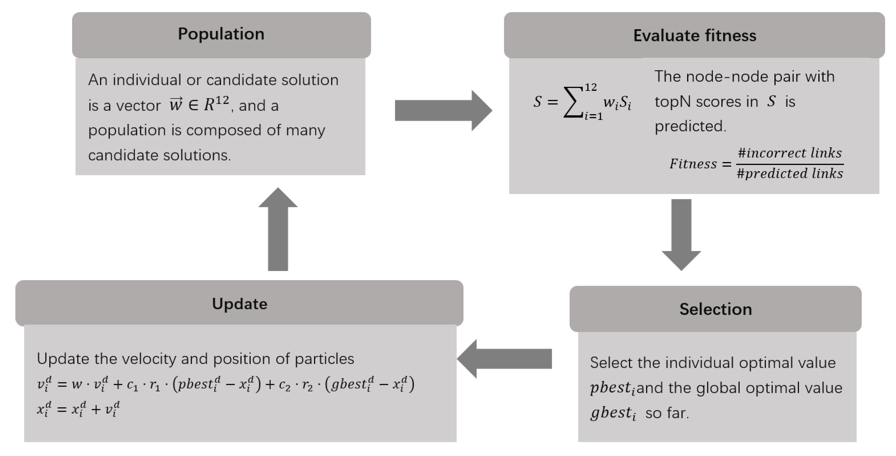
Experimental Evaluation Methods and Results
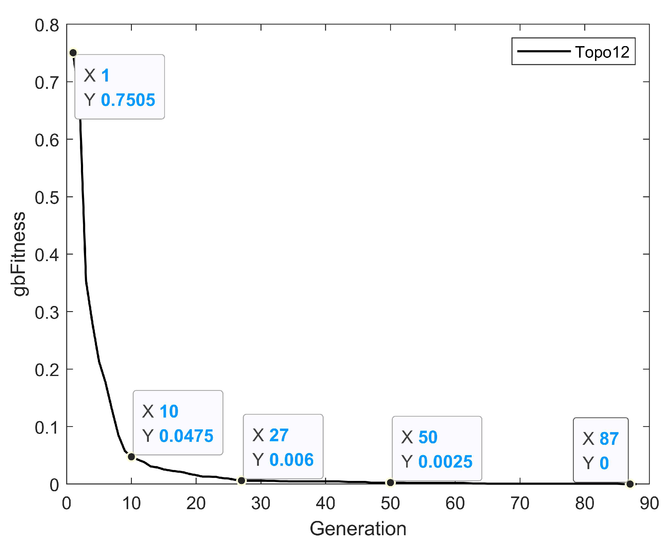
Figure 3 shows the fitness20 (topN = 20) results of new links formed during the training period from 1986 to 1987. The black solid line depicting the “Topo12” predictor shows that the average optimal fitness value of 100 candidate solutions dropped sharply from 0.7505 to 0.0475 within 10 generations, and then eased slightly, and dropped to 0.006 by the 27th generation. In the 50th generation, it was reduced to 0.0025. After that, the line was getting closer and closer to the X-axis. By the 87th generation, it completely coincided with the X-axis, and the average optimal fitness value reached a satisfactory result of 0. The curves are consistent with the characteristics that the particle swarm optimization algorithm converges quickly at the beginning of the iteration and slowly at the end, and the overall convergence is relatively fast. In fact, the optimal fitness value converges to 0 much earlier in most runs, but the image depicts the average result over 100 runs, and because the particle swarm algorithm has the disadvantage of easily falling into local optima late in the process, several of these runs take far more generations than normal to reach a fitness value of 0, thus lengthening the number of generations required for the overall average.
To better understand the performance of each topological similarity index in the employed link predictor, we plotted
Figure 4 to visualize this aspect of information.
Figure 4 shows all 100 solutions obtained by evolving the particle swarm optimization algorithm in parallel with Spark for 250 generations, where
is used as the horizontal row. The i-th column represents the coefficients of
used for the linear combination, and the color of the axes indicates the position where the coefficient values are located. It can be observed from the images that the 100 candidate solutions differ significantly from each other. Nevertheless, we can still find more positive than negative values for the Average Path Weight and Katz, with the former accounting for more than 90% of the positive values and the latter not even having any negative values, while Preferential Attachment is basically all negative with only two sporadic positive values. This means that for a high-scoring author pair, if it contains a large number of positive weights for Average Path Weight and Katz and a large number of negative weights for Preferential Attachment, then a link between the two authors will be more likely to be generated in the future, that is, more likely to collaborate.
The ranking frequencies of each similarity index were visualized according to their coefficients, as shown in
Figure 5. The coefficients are ordered from the most positive (in first place) to the most negative (in 12th place). As can be seen from the images, Average Path Weight and Katz frequently occupy the first to fourth positions in the ranking, while the Hub-promoted Index, Hub-depressed Index, Leicht-Holme-Newman Index, Salton Index, and Sorenson Index ranked 8th to 12th most frequently. The other indices were relatively dispersed.
Since the positive class is much smaller than the negative class in large sparse networks, given this imbalance, even for random link predictors, metrics such as accuracy and negative predictive value are very close to 1. Therefore, this paper puts more attention on recall and accuracy, which are shown in Equations (5) and (6), respectively, and Equation (
7) is a combined metric
that combines the two.
is used to adjust the weight of recall and accuracy—when
both weights are the same, if the accuracy is considered more important then
is reduced, and if recall is considered more important then
is increased accordingly.
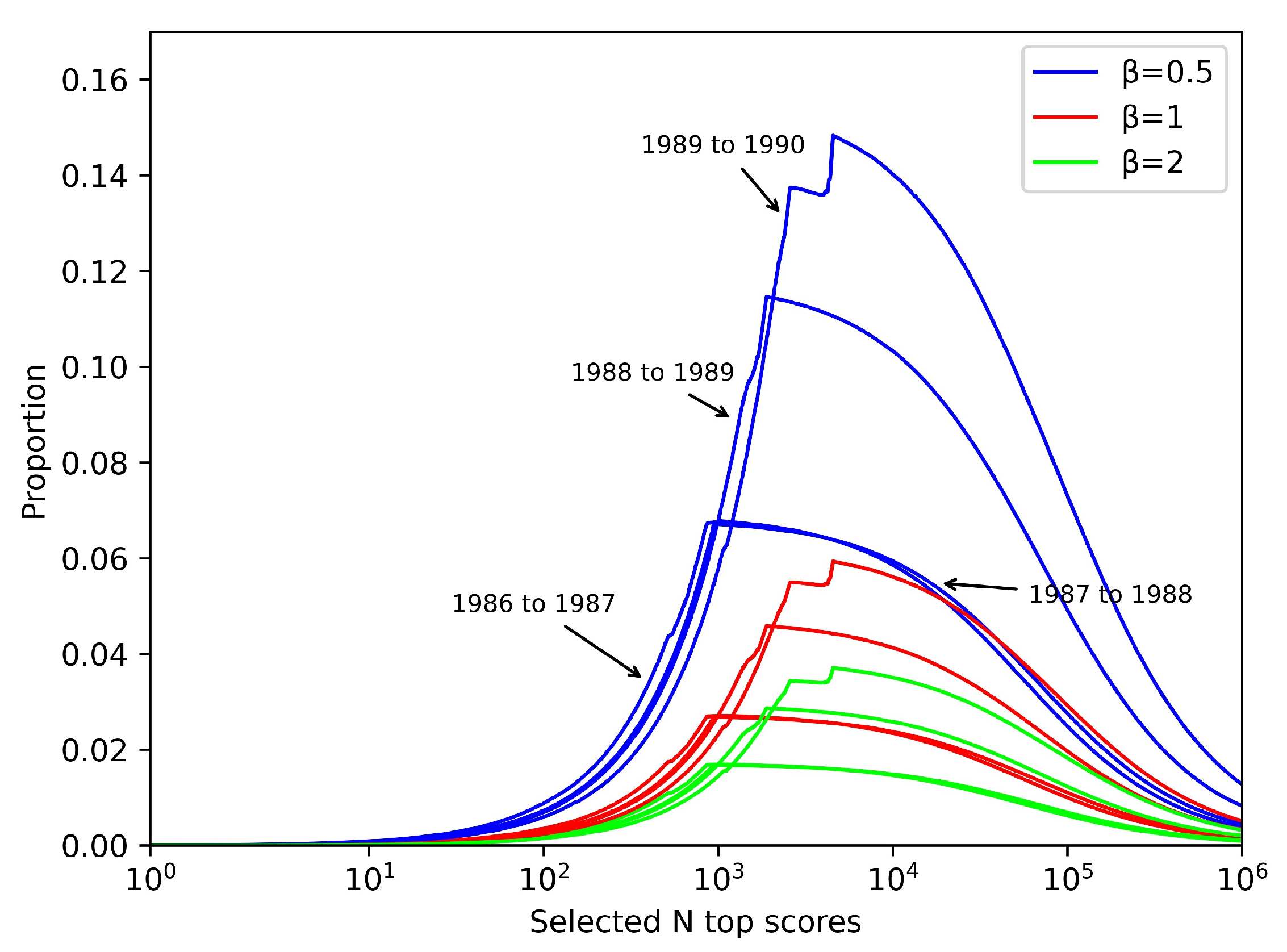
Adjusting
to one of 0.5, 1, and 2, respectively and plotting
Figure 6, it is easy to find that
reaches its extreme value roughly at
. Since the number of selected academic network collaborator nodes increases with the year, the corresponding number of node–node pairs of links consisting of any two authors also increases with the year with a difference of hundreds of millions or more. It is observed that for years with a higher number of links, the
value is also clearly higher.
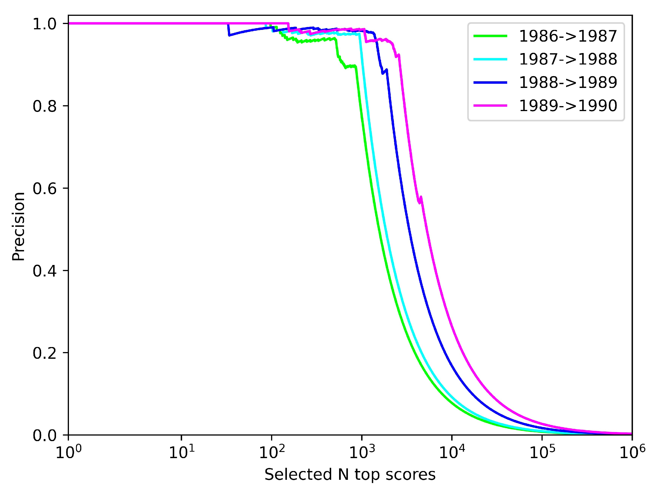
Figure 7 depicts the precision of the link prediction under the top N-scoring author–author pairs. It is not difficult to find that the fitness function of the algorithm runs achieves essentially zero-error precision across the validation sets when scoring author–author pairs below about
are selected, and extremely high precision between
and
. After that, the curve plummets from smallest to largest by validation set year, mainly because all correctly predicted links have been basically identified until N is about
, and increasing N further just increases the false-positive rate in vain. Overall, it can be seen that our prediction of co-authorship works well.


