RDFsim: Similarity-Based Browsing over DBpedia Using Embeddings

Abstract

Browsing has been the core access method for the Web from its beginning. Analogously, one good practice for publishing data on the Web is to support dereferenceable URIs, to also enable plain web browsing by users. The information about one URI is usually presented through HTML tables (such as DBpedia and Wikidata pages) and graph representations (by using tools such as LODLive and LODMilla). In most cases, for an entity, the user gets all triples that have that entity as subject or as object. However, sometimes the number of triples is numerous. To tackle this issue, and to reveal similarity (and thus facilitate browsing), in this article we introduce an interactive similarity-based browsing system, called RDFsim, that offers “Parallel Browsing”, that is, it enables the user to see and browse not only the original data of the entity in focus, but also the K most similar entities of the focal entity. The similarity of entities is founded on knowledge graph embeddings; however, the indexes that we introduce for enabling real-time interaction do not depend on the particular method for computing similarity. We detail an implementation of the approach over specific subsets of DBpedia (movies, philosophers and others) and we showcase the benefits of the approach. Finally, we report detailed performance results and we describe several use cases of RDFsim.

1. Introduction

There are several access methods over RDF knowledge bases, which can be divided in structural query language methods, such as SPARQL (https://www.w3.org/TR/sparql11-query/, accessed on 21 October 2021), keyword search methods, such as [1,2], interactive information access methods (e.g., [3,4]), and natural language interfaces (e.g., [5]), see Figure 1 for an overview.

The category of interactive information access services, aims at aiding users to browse and/or interactively formulate queries in a user friendly manner. This includes plain browsing of web pages that, for each entity URI, present all triples of that URI as HTML tables; see for example the pages for Aristotle in DBpedia (https://dbpedia.org/page/Aristotle, accessed on 21 October 2021) and Wikidata (https://www.wikidata.org/wiki/Q868, accessed on 21 October 2021). This category also includes faceted search systems [6,7] and interactive query formulators for RDF data like A-Qub [8].

In this paper, we focus on browsing, since this is a generic interactive access mechanism. Sometimes the number of triples of an entity is big, thereby it can result in information overload; for example, the webpage about Aristotle in DBpedia [9] contains over 1000 links (!), making it hard for the user to identify the most important information. To alleviate this problem in this paper, we investigate a similarity-based browsing method for RDF data, that allows a user to see only the K most similar entities, offering in this way a method to tackle the information overload. Instead of designing manually a similarity function for RDF, we exploit knowledge graph embeddings [10], since they could capture similarity more accurately. Apart from tackling information overload, a similarity-based browsing approach can show to the user entities which are not necessarily directly connected with the current entity. For instance, the page of Socrates (https://dbpedia.org/page/Socrates, accessed on 21 October 2021) in DBpedia does not include a link to Homer (https://dbpedia.org/page/Homer, accessed on 21 October 2021), and vice versa; however, the similarity-based algorithm which is used in this article (more details are described later) detected these two famous people from Ancient Greece as similar.

Although there are various similarity-based services for RDF data, such as KGvec2go [11] and LODVec [12], where one can find the K most similar entities to a given URI and the similarity between two different URIs (concepts), to the best of our knowledge there is no browsing system for RDF data that supports similarity-based browsing (the current browsing systems [3,4,13] do not support such similarity services).

To support similarity-based browsing, several questions arise, including: (a) how to present the most similar entities to a given entity; (b) what kind of interaction with these entities to support; and (c) what kind of indexes are required to enable real-time interaction (without being dependent on the particular method that is used for computing similarity).

In this paper, we introduce an interactive similarity-based browsing system, called RDFsim, that offers “parallel browsing”, that is, it enables the user to see and browse not only the original data of the entity in focus, but also the K most similar entities of the focal entity in the form of a star-like graph or tagcloud. For example, Figure 2 shows the default browsing system for the entity “Socrates”: the left frame contains its Wikipedia page, while the right shows the top-K (default K is 10) similar entities in the form of a graph, and the user can interact with any of these two frames to change the entity in focus. The similarity of entities is founded on knowledge graph embeddings. In particular, RDFsim currently applies the word2vec model [14,15] for computing the embeddings (vectors) for a set of URIs (i.e., entities), and uses the cosine similarity metric for computing the similarity between the vectors of two URIs. To enable real-time interaction, which is indispensable for browsing, we propose and evaluate dedicated indexes that do not depend on the particular method for computing similarity. The current version of RDFsim is publicly available (https://demos.isl.ics.forth.gr/RDFsim/, accessed on 21 October 2021) and offers similarity-based browsing for over 350,000 entities of DBpedia. Regarding evaluation, we compare RDFsim with existing browsing systems, and we report detailed performance results. Finally, we discuss use cases that showcase the benefits of the approach through some real scenarios.

The rest of the paper is organized as follows: Section 2 describes the related work, Section 3 describes the process of RDFsim for computing and storing the top-K similar entities using embeddings, whereas Section 4 introduces the process of “Parallel Browsing”. Section 5 compares the approach with related browsing systems, provides statistics about the datasets supported by RDFsim, and reports performance results. Section 6 discusses use cases that involve RDFsim, and finally Section 7 concludes the paper and identifies directions and issues that are worth further research.

2. Related Work

In this section, we discuss access systems for RDF (in Section 2.1), semantic similarity methods by focusing on systems that exploit RDF knowledge graph embeddings (in Section 2.2), and the positioning and novelty of RDFsim (in Section 2.3).

2.1. Access Systems over RDF

The access methods over RDF can be categorized as: (a) Structured Query Languages, (b) Keyword Search, (c) Interactive Information Access, and (d) Natural Language Interfaces. This categorization and the characteristics of each case are shown in Figure 1.

Concerning (a), by accessing RDF through query languages such as SPARQL (https://www.w3.org/TR/sparql11-query/, accessed on 21 October 2021), it is feasible to express complex queries through precise and complex criteria. Such languages return exact match results and offer multi-column responses. There are several systems available offering data storage and query processing (see a survey [16] for more details). However, they are more applicable for users that are familiar with such language. Regarding (b), there exists keyword search approaches [17], where one can submit a set of keywords, and they return as output the best match entries, which are produced by a sophisticated ranking. These approaches use several techniques for retrieving the best match results, by exploiting Information Retrieval (IR) techniques [18,19], and/or by adapting existing IR systems, like Elasticsearch, to the needs of RDF, for example, see [1,2,20] and others. As regards (c), there are several interactive information access systems, including browsing systems, such as [3,4,21] and also systems that can aid users that are not familiar with query languages to access the RDF knowledge base, for example, faceted search [6,7,13], interactive analytics services [22,23] and also systems for assisting the query building process, such as the system A-Qub [8]. Finally, regarding (d) Natural Language interface systems [24], where the input and output is given in natural language, and it returns short and precise answers, that is, through conversational access and Question Answering systems [25,26,27,28].

2.2. Semantic Similarity Methods (Focus on RDF Knowledge Graph Embeddings)

According to [29], there exist several semantic similarity methods, which can be divided into four categories: (I) knowledge-based methods, that is, “they calculate semantic similarity between two terms based on the information derived from one or more underlying knowledge sources, such as ontologies/lexical databases, and others”, (II) corpus-based similarity methods, that is, “they measure semantic similarity between terms using the information retrieved from large corpora, such as word embeddings”, (III) deep neural network techniques, which exploit state-of-the-art neural networks models for improving performance, and (IV) hybrid methods, which combine methods from at least two of the previous categories.

2.2.1. Semantic Similarity in Knowledge Bases

The notion of similarity in knowledge bases (Category I), for example, in RDF knowledge bases, has been studied over the past decades, since it is of primary importance for identifying objects that are similar, but not equivalent. In general, the similarity between two elements of a Knowledge Base can have several aspects, for example, lexical similarity (two elements have the same or close name), connectional similarity (they are connected to the same or similar entities), structural similarity (they have topologically similar structure), type similarity (they belong to the same/close types, that is, classes), and of course one can devise similarity measures that capture two or more of the above aspects.

Just indicatively, the authors of [30] proposed a framework for assessing semantic similarity among instances of a given ontology, while the idea for similarity-based browsing for Linked Data was first proposed in [31], where the similarity between two entities is computed based on similarities between the subgraphs of these entities (however, that work was not applied on large knowledge bases).

2.2.2. RDF Knowledge Graph Embeddings

There is a recent trend for creating RDF knowledge graph embeddings for computing similarities [10,32]. With respect to the categorization discussed in Section 2.2, such methods are essentially hybrid since they combine techniques from both Categories I and II. Specifically, they exploit corpus-based methods for computing the embeddings for RDF knowledge graphs (instead of texts). In these approaches, the way that sentences are produced from the KB determines the derived corpus over which the embeddings will be produced, hence this (i.e., the sentence production) determines what the embeddings-based similarity really captures. In our case (as it is described in detail in Section 3.2), for an entity we produce one sentence for each of its triples; consequently, the similarity that it is calculated is based on the co-occurrence of classes, properties and property-values.

Concerning services exploiting RDF knowledge graph embeddings, KGvec2go [11] offers an API by exploiting the embeddings trained on four different RDF knowledge graphs by using the RDF2Vec model [10]. In particular, one can find the similarity between two different concepts, the K closest concepts to a given one and so forth. Furthermore, Wembedder [33] is a system that provides the most similar entities for a Wikidata entity through a web application and a REST API. Moreover, LODVec [12,32] is a tool that can produce URI sequences and embeddings for a set of given entities, by exploiting the indexes of LODsyndesis knowledge graph [34]. The main difference between the mentioned tools and RDFsim is that RDFsim mainly focuses on browsing (and not only on offering a similarity API).

2.3. The Positioning and Novelty of RDFsim

Concerning access methods, RDFsim belongs to category (c), since it offers an interactive information access system for aiding the user to find similar entities for one or more URIs (i.e., entities), without requiring from the user to be familiar with query languages (e.g., SPARQL), nor with the contents of the dataset. Regarding similarity methods, it belongs to the category of RDF knowledge graph embeddings, that is, it supports functionality similar to the one offered by systems such as KGvec2go [11], Wembedder [33] and LODVec [12,32], since all these tools can provide the most similar entities to a given one.

Concerning the novelty of RDFsim, to the best of our knowledge RDFsim is the first browsing system over Knowledge Bases that offers “parallel browsing” (full contents and top-K entities), and is equipped with dedicated indexes enabling real-time browsing, and size-configurable visualization methods. The detailed performance experiments and the online demo showcase the feasibility and generality of the approach.

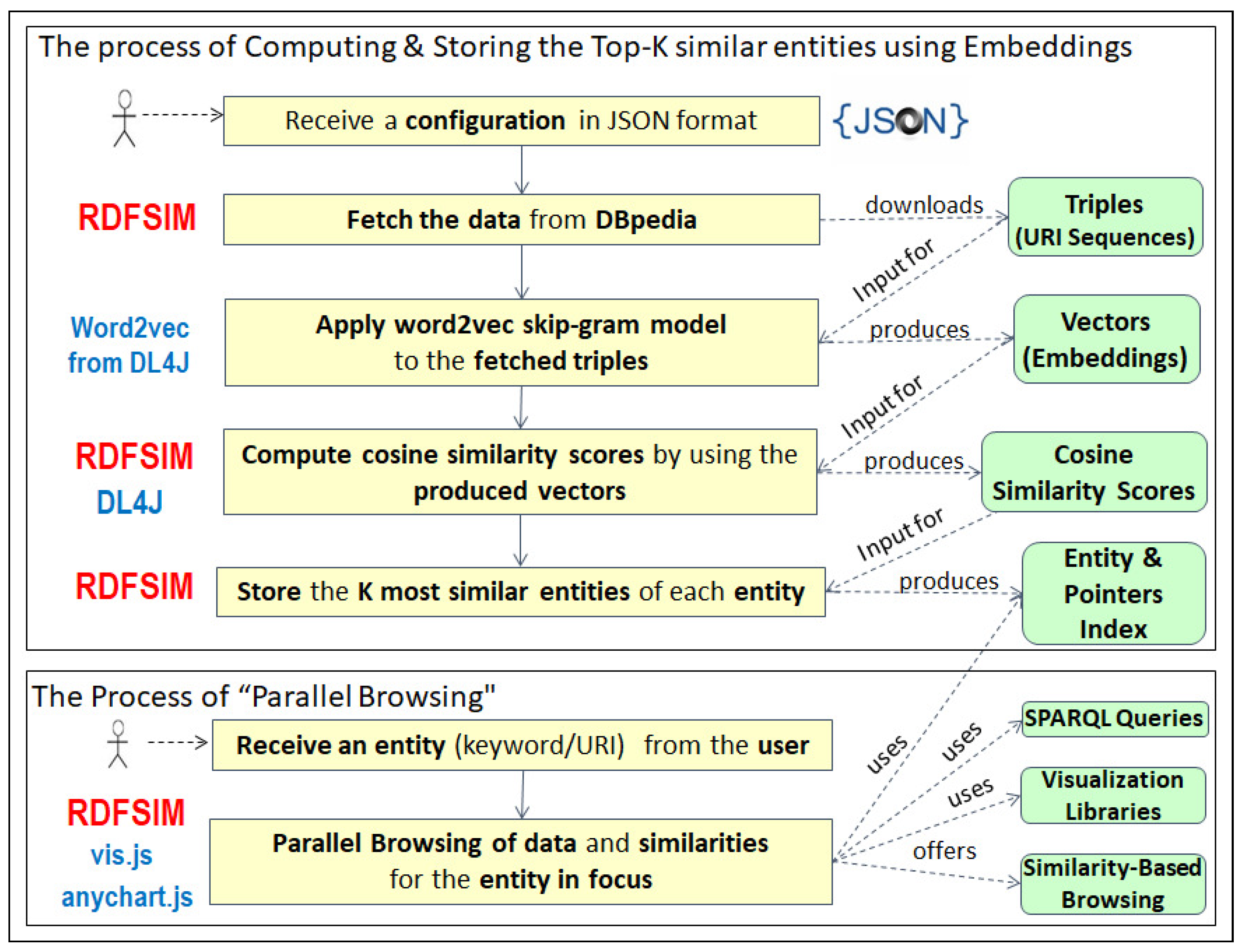
3. The Process of Computing and Storing the Top-K Similar Entities Using Embeddings

Here, we describe the first part of RDFsim process, which is illustrated in the upper part of Figure 3. In particular, we introduce the three steps, for downloading the desired data from DBpedia (Section 3.1), for computing the top-K similar entities through embeddings (Section 3.2), and for storing the results in dedicated indexes (Section 3.3). These steps are described in Algorithm 1, whereas Figure 4 shows a running example, where we create the embeddings for the entities belonging to the DBpedia class of “Philosophers”.

Algorithm 1: Creating the Entity and the Pointers Index, by using the embeddings created from the data of a SPARQL query to DBpedia.

Input: Input query q for downloading the triples from DBpedia SPARQL endpoint Output: The entity Index $ei$ containing for each entity its prefix, its URI and its top-K similar entities, and the pointers index $pi$   /*$\phantom{(}$ Step A. Download the triples by using the input query q$\phantom{(}$     */  1 $triples\leftarrow downloadDBpediaTriples\left(q\right)$  /*$\phantom{(}$ Step B. Create the embeddings (vectors) for the URIs of the fetched triples by using word2vec $\phantom{(}$     */  2 $vecMap\leftarrow word2vec.skipgram\left(triples\right)$  //$\phantom{(}$ Step C. Create the Indexes by using the produced vectors $\phantom{(}$  3 $EntityIndexei\leftarrow \varnothing$  //$\phantom{(}$ Read each URI of $vecMap$ for creating the Entity Index $\phantom{(}$  4 forall $uri\in Left\left(vecMap\right)$ do$\phantom{(}$  5    $entity\leftarrow suffix\left(uri\right)$    //$\phantom{(}$ The top-K most similar entities to $uri$ wrt $cos{\left(\theta \right)}_{uri,ur{i}^{\prime }}$ score  6    $\phantom{(}$$similars(entity,K)\leftarrow getSimilarEntities(uri,vecMap,K)$    //$\phantom{(}$ Store the above information to the index $\phantom{(}$  7    $ei\leftarrow ei\cup \left\{\right\{entity,uri,similars(entity,K)\left\}\right\}$  8  $ei\leftarrow ei.sortBySuffixLexicographically\left(\right)$  //$\phantom{(}$ Create the Pointers Index by using the Entity Index $\phantom{(}$  9 $PointersIndexpi\leftarrow createPointersIndex\left(ei\right)$  10 Return $ei$,$pi$

3.1. Step A. Configuration and Data Fetching

Rationale. RDFsim downloads data from DBpedia knowledge base [9]. We decided to use DBpedia since it offers the following benefits: (a) it covers several domains since it depends on Wikipedia, (b) it provides human readable URIs, that is, the suffixes of its URIs (the last part of URIs) provide information about the entity being described, whereas other cross-domain datasets use identifiers as suffixes (e.g., Wikidata), and (c) it offers deferenceable URIs, that is, by clicking to a URI, one is redirected to its corresponding page of DBpedia.

The process. The configuration is given in JSON format and should at least include the SPARQL query for downloading the data from DBpedia. Moreover, the configuration can include parameters needed for the computation of the embeddings, for example, the number of dimensions for the vectors to be produced, the minimum frequency of a word, and others. Concerning Data Fetching, RDFsim downloads the data by sending SPARQL queries to DBpedia SPARQL endpoint (https://dbpedia.org/sparql, accessed on 21 October 2021) and stores them locally in Ntriples format, that is, see line 1 of Algorithm 1. In our running example (Figure 4), the input is all the triples containing entities of the class “Philosophers” either as a subject or as an object, whereas these triples contain only URIs. The corresponding SPARQL query is the following:

3.2. Step B. Production of Embeddings for the Fetched Data and Computation of Similar Entities

Rationale. The target is to create a single multidimensional vector for each URI occurring in the fetched data.

Word2vecmodel. To generate these vectors, we exploit word2vec, a shallow two-layer neural network model that uses a single hidden layer for producing word embeddings [14,15]. The input is a text (in our case triples), while the output is a multidimensional vector (usually with over a hundred dimensions) for each unique word (in our case URI) that appears in the text. The vectors it produces are based on the co-occurrence of words (in our case URIs) in context windows of a given size, and it aims at grouping the vectors of similar words (based on their co-occurrence) closely in the vector space. The recommended value of the size of the context window depends on the word2vec model, for example, in the skip-gram model (which is used by RDFsim), that value is usually around 10. However, in our case we use a context window of size 3, since for an entity we produce one sentence for each of its triples (i.e., each sentence contains 3 URIs), which means that we capture similarities based on the co-occurrence of classes, properties and property-values. The methods for computing the vectors and the similarity scores are detailed in Section 3.2.1 and Section 3.2.2.

Word2vecand alternative options. Although there are several methods for producing word embeddings, in this work we started from word2vec, since it has been successfully used over the past years for a large variety of similarity-based applications (e.g., for the task of entity relatedness and for machine learning-based tasks) over RDF knowledge bases (including DBpedia), for example, see [10,32]. However, later in this paper (in Section 3.4), we describe how the proposed approach could be adjusted for hosting similarity results that are produced by other similarity methods as well.

3.2.1. Step B1. Computation of URI Embeddings

Here, we describe the text corpus that we use and the process that is followed for computing the embeddings.

Text Corpus. We do not use any pre-trained word2vec vocabulary for computing the embeddings. In particular, our text corpus is derived by the input triples (from Step A), and we train the model by using the mentioned triples. We consider each URI, for example, “dbp:Aristotle” or “dbp:Western_Philosophy”, as a single word, and we consider each RDF triple as a sentence (a sequence of URIs), for example, “dbp:Aristotle, dbp:bornIn, dbp:Stagera” is a URI sequence containing three URIs. At the time being, we use triples containing only URIs (see Step B1 of Figure 4), and not triples including literals or blank nodes, since such cases require a more complicated approach (e.g., more details are given in [35]), we plan to investigate such cases in the future.

Skip-gram model. For computing the embeddings, we use the skip-gram model of word2vec [14,15]. We decided to use this model instead of the Continuous-Bag-of-Word (CBOW) model of word2vec, since in most cases Skip-gram outperforms CBOW for large RDF datasets (including DBpedia) [10,32]. Skip-gram model uses unsupervised learning techniques for finding the most related words (in our case URIs) for a given word, that is, it uses a target word for predicting the context words. For instance, in the upper right side of Figure 4, the target URI is “dbp:Aristotle” and some of the context URIs (for “dbp:Aristotle”) are “dbp:Plato” and “dbp:Thales”.

In particular, given a sequence of training URIs (words), say $ur{i}_1,ur{i}_2,...,ur{i}_T$, and a context window of size c, the skip-gram model tries to maximize the average log probability, which follows:

$$\frac{1}{T}\sum _{t=1}^T\sum _{-c\le j\le c,j\ne 0}^{}logp\left(ur{i}_{t+j}\right|ur{i}_t).$$

(1)

The probability $p\left(ur{i}_{t+j}\right|ur{i}_t)$ is computed using the softmax function:

$$p\left(ur{i}_{t+c}\right|ur{i}_t)=\frac{exp\left({v\prime }_{ur{i}_{t+c}}^T{v}_{ur{i}_t}\right)}{{\sum }_{m=1}^{\left|U\right|}exp\left({v\prime }_{ur{i}_m}^T{v}_{ur{i}_t}\right)}.$$

(2)

In the above formula, $v^{\prime }$ and v are the input and the output vectors of a URI $uri$, whereas $\left|U\right|$ is the number of unique URIs in our vocabulary (text corpus).

3.2.2. Step B2. Production of Vectors for the URIs and Computation of Similar Entities

After the training phase, each URI $uri$ is mapped into a vector $v_{uri}^{\prime }$ (see line 2 in Algorithm 1), and we store all these vectors. In particular, we use a map, called $vecMap$, which is essentially a function $vecMap:U\to VEC$, where U denotes all the trained URIs, $VEC$ all the produced vectors, and $vecMap\left(uri\right)=v_{uri}^{\prime }$ (e.g., see Step B2 of Figure 4). The key point is that semantically similar URIs are placed to close positions in the vector space, for example, see an example in Step B2 of Figure 4 for the URIs “dbp:Aristotle”-“dbp:Plato” and the URIs “dbp:Western_Philosophy”-“Ancient_Greek_Philosophy”.

We should note that the URIs (in our vocabulary) can belong to different RDF classes, that is, “dbp:Aristotle” belongs to the class of “dbo:Philosopher”, while “dbp:Stagera” belongs to the class of “dbo:City”. Therefore, it is possible for entities belonging to different classes, such as “dbp:Aristotle” and “dbp:Stagera”, to be detected as similar through Skip-gram model.

Similarity Method for computing the K most similar entities. For finding the K most similar entities to a given entity, we employ the cosine similarity score of their vectors. The cosine similarity between two vectors $v_{ur{i}_1}^{\prime }$ and $v^{\prime }\left(ur{i}_2\right)$ (each vector correspond to a single URI) is defined as:

$$cos{\left(\theta \right)}_{ur{i}_1,ur{i}_2}=\frac{v_{ur{i}_1}^{\prime }·v_{ur{i}_2}^{\prime }}{\parallel v_{ur{i}_1}^{\prime }\parallel \parallel v_{ur{i}_2}^{\prime }\parallel }.$$

(3)

The score ranges from -1 (i.e., two vectors are exactly opposite) to 1 (i.e., two vectors are exactly the same). To compute the K most similar entities to a given URI $uri$, we rank the rest URIs according to their $cos{\left(\theta \right)}_{uri,ur{i}^{\prime }}$ score in descending order, and we keep the URIs placed in the first K positions in the ranking (i.e., the K most similar URIs to $uri$).

Implementation. For the computation of embeddings and of the cosine similarity scores between the URIs, RDFsim uses the word2vec DL4J API (https://deeplearning4j.org/, accessed on 21 October 2021).

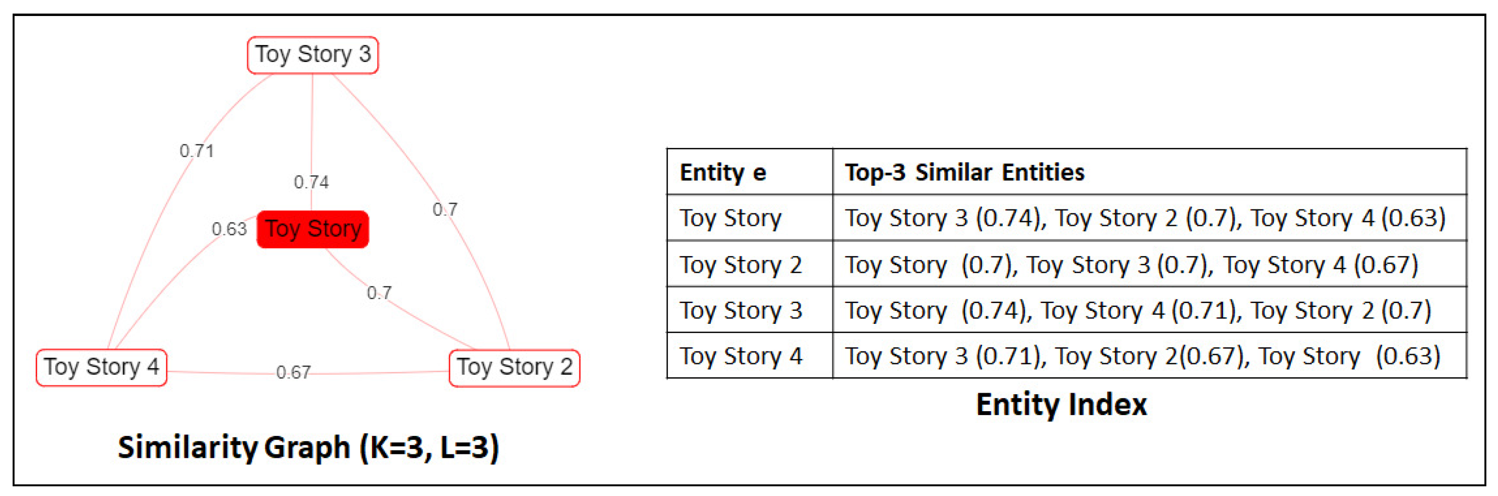
3.3. Step C. The Indexing Process

Rationale. The computation of embeddings and of similarity scores between the URIs usually need high main memory requirements. To support fast browsing and avoid recomputing similarity scores we store the top-K similar entities of each entity in specialized indexes. Afterwards, we use only these indexes for offering “parallel browsing”, that is, there is no need to store (either in main memory or on disc) the produced embeddings (i.e., computed in Step B). Therefore, for tackling performance requirements and for offering real-time interaction, we create the following two indexes: (a) the Entity Index and (b) the Pointers Index, that is, see lines 3–10 of Algorithm 1.

Entity Index. It is a Random Access file containing a single entry for each URI (or entity), by exploiting the results of the embeddings. The process is described in lines 3–8 of Algorithm 1. Firstly, we read each URI (see line 4) for which a vector was produced in the previous step (with $Left\left(r\right)$ we denote the set of elements that occur in the left side of a function r). Afterwards, for each URI (i.e., entity), we store as a key its suffix (i.e., the last part of the URI), the whole URI, its top-K similar entities (i.e., $similars(e,K)$ in line 6 of Algorithm 1), and their corresponding similarity score (computed by using the vectors of $vecMap$ and the cosine similarity metric). An example can be seen in the lower side of Figure 4, where we have stored the above information for some entities. The top-K similar entities of each entity are stored in descending order according to their cosine similarity score, whereas the entities of Entity Index are stored in lexicographical order (according to their suffix).

Pointers Index. For being able to offer faster responses, we use this index for creating some pointers to specific positions of Entity Index (see lines 9–10 of Algorithm 1). Indeed, Pointers Index can store a single pointer for a specific word prefix. Since Entity Index has been sorted in lexicographical order, it can store a pointer according to a given policy, for example, for each distinct character, for the first two characters, and so forth, as in [36], depending on the scalability requirements. For example, in our running example of Figure 4, the pointer of the letter ’A’ points to the first entity whose suffix starts with ’A’. These indexes are exploited for offering “Parallel Browsing”, as is described in Section 4.

3.4. How Can the Process Be Adjusted to Other Datasets or Similarity Methods?

The described process can be easily adjusted to datasets having suffixes containing a surface form of the concept, such as DBpedia. On the contrary, for other datasets, such as Wikidata, which use identifiers as suffixes, one possible solution is to perform the same process in Steps A and B, and afterwards to store in the index the label of each URI, instead of its suffix. Our plan is to investigate methods for supporting this kind of dataset in the future.

Concerning different methods for computing similarity, it is worth noting that the produced index stores the K most similar entities to a given entity, that is, the index does not depend on the particular method for computing similarity. Therefore, one could use the indexes of RDFsim for storing the similar entities as computed by different embeddings models, such as BERT [37], GloVE [38], FastText [39], and others. In such scenarios, steps A and B could be skipped and the precomputed similarity results could only be used for producing the indexes.

4. The Process of “Parallel Browsing”

This section describes the second part of the RDFsim process (lower part of Figure 3), that is, the process of “Parallel Browsing” that enables the user to browse both the original data of the focal entity, and the K most similar entities of that entity. To enable real time interaction, this process exploits the indexes produced in Step C (Section 3.3). In brief, Section 4.1 describes the selection of the first entity, Section 4.2 describes the frames, Section 4.3 describes the methods/algorithms used for retrieving and visualizing the data, and Section 4.4 provides details about the implementation and the current version of RDFsim.

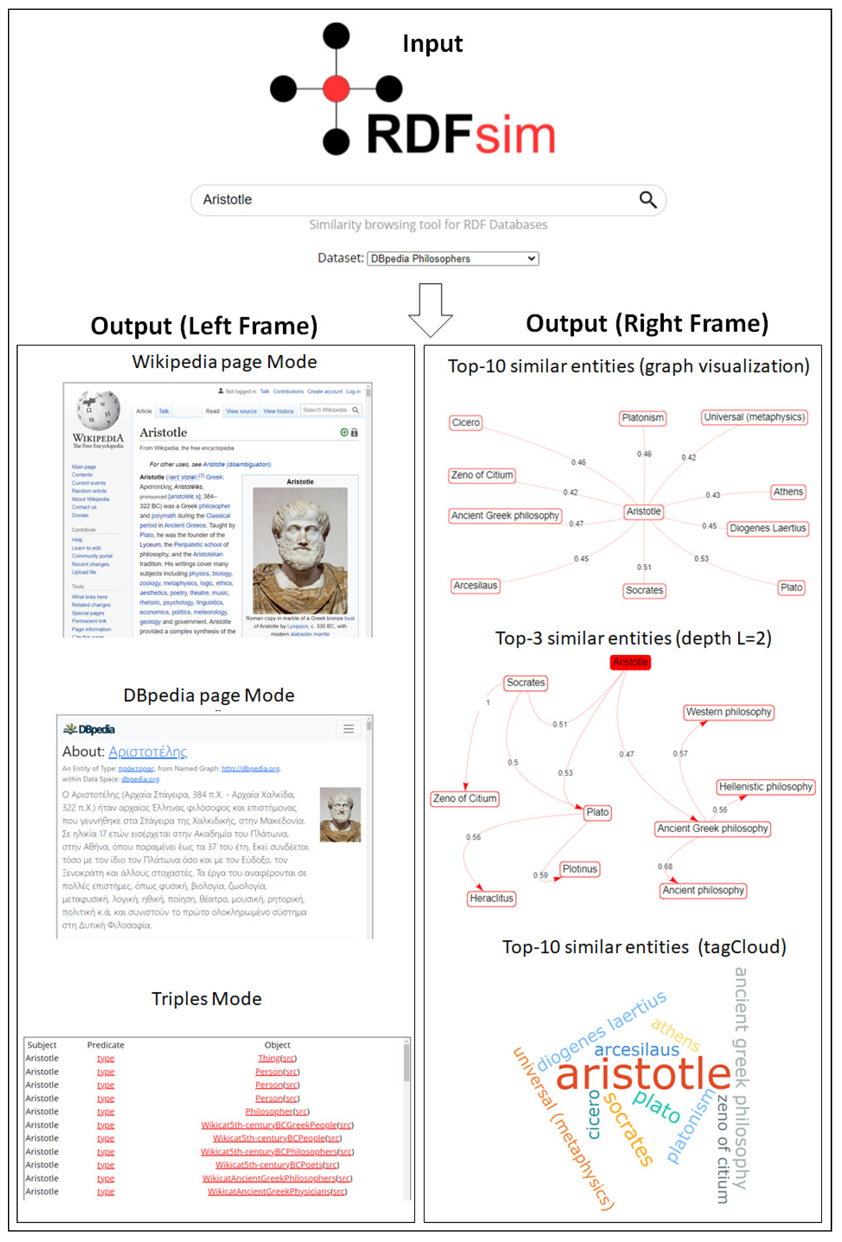
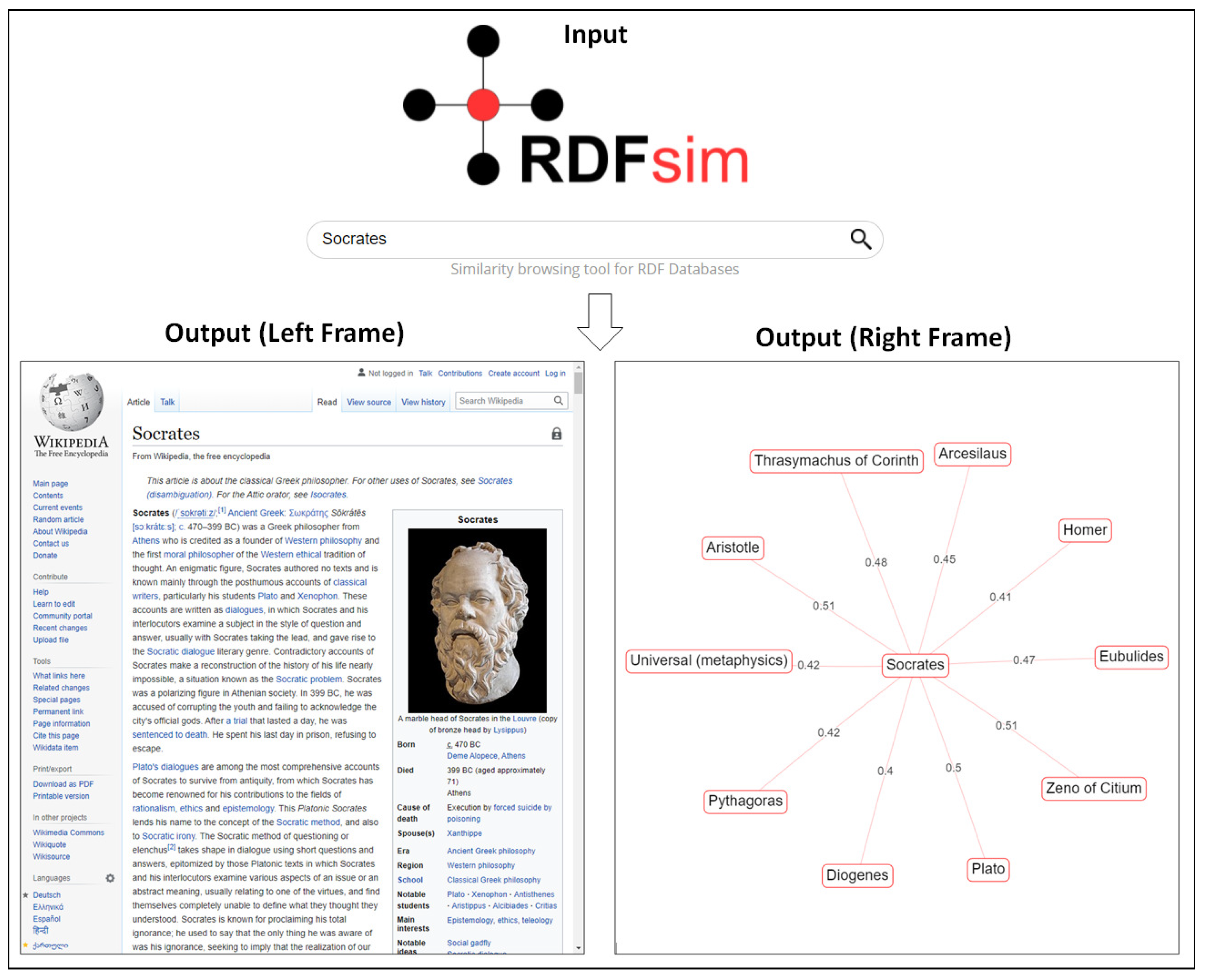
4.1. Landing Page and Finding the First Entity

The first page of RDFsim web application contains a search form, where the user can type either a URI or a keyword which corresponds to an entity, whereas through a select box the user can select which dataset to use (e.g., “Philosophers”,“Movies”, etc). To aid users in finding the desired entity, RDFsim offers an auto-complete mechanism. An example is shown in the upper side of Figure 5, where the input keyword is “Aristotle” and the selected dataset is “DBpedia Philosophers”.

4.2. The Frames of “Parallel Browsing”

After selecting the focal entity $e_{sel}$, the user is redirected to a new page, where “Parallel Browsing” is offered for that entity. This page is divided into two different frames (or parts), as is depicted in Figure 5. In the left frame, RDFsim shows the original data of $e_{sel}$, in three possible modes: (i) Wikipedia page mode (default), where the user explores the Wikipedia page of $e_{sel}$, (ii) DBpedia page mode, where the user browses the DBpedia page of $e_{sel}$, and (iii) triples-mode, where the user can browse all the triples where $e_{sel}$ occurs either as a subject or as an object. In the right frame, the user can see the top-K (K is configurable) most similar entities to $e_{sel}$ through either a graph visualization (e.g., see the graphs in Figure 5) or a tagCloud visualization (e.g., see the lower right side of Figure 5).

By clicking to an entity either in the left frame (only in triples mode) or in the right frame, RDFsim will refresh the page for showing the corresponding information for the new selected entity.

4.3. Constructing the Browsing Frames

Here, we describe the methods for retrieving the data for the selected entity $e_{sel}$, and for constructing the two browsing frames.

4.3.1. Finding the Selected Entity in the Index

Since in our index we store the entities according to their suffix, in case that the input is a URI, we just keep its suffix. Afterwards, we use the Pointers Index for retrieving the entity $e_{sel}$ from the Entity Index. In our running example, where $e_{sel}=$“Aristotle”, we find its first letter (i.e., ‘A’), we find the pointer of this character in the Pointers Index, and we read the Entity Index starting from that pointer for finding $e_{sel}$. For offering faster responses, we use binary search for finding and retrieving the line containing the data of the given entity.

4.3.2. Constructing the Left Frame of RDFsim Web Page

For any selected mode of the left frame, we retrieve from the Entity Index only the URI of $e_{sel}$. For Wikipedia or DBpedia page mode, we use that URI for finding the corresponding URL of that pages and for showing them to the left frame of RDFsim. On the contrary, for the triples mode, we send a SPARQL query to DBpedia SPARQL endpoint for retrieving dynamically all the triples containing the URI of $e_{sel}$ either as a subject or as an object.

4.3.3. Constructing the Right Frame of RDFsim Web Page

The right frame of the web application supports two visualizations for the similaritybased browsing, which are analyzed below.

A. Similarity Graph Visualization.RDFsim constructs a similarity graph for visualizing the K most similar entities to $e_{sel}$ and the cosine similarity score between the URI of $e_{sel}$ and the URI of each similar entity of $e_{sel}$. Moreover, it can construct larger similarity graphs by using a parameter L, which denotes the maximum depth that the graph can have, that is, the number of edges in the longest path of the graph. For a given L ($L\ge 1$), the graph contains at most $L+1$ levels, where the first level contains the selected entity $e_{sel}$, the second level the top-K most similar entities of $e_{sel}$, that is, $similars(e_{sel},K)$, the third level the top-K similar entities of each similar entity of $e_{sel}$, that is, $similars(e^{\prime },K)$, where $e^{\prime }\in similars(e_{sel},K)$, and so forth.

The default values are $K=10$ and $L=1$, that is, the graph contains the top-10 similar entities for the selected entity $e_{sel}$ (see the first graph in the right side of Figure 5). On the contrary, by increasing the value of L, one can browse more complex similarities, for example, to see which entities belong to the top-K similar entities for both “Aristotle” and “Socrates” (see the second graph in the right side of Figure 5). Below, we describe how to construct such graphs.

Construction of Similarity Graph. For constructing this graph we use a Breadth-First Search (BFS)-like algorithm (see Algorithm 2), which is analyzed below.

Input. It receives as input the selected entity $e_{sel}$ and two parameters, that is, K (the number of the top-K most similar entities) and L (the maximum depth of the graph).

Output. The output is a similarity graph G having a depth of at most L, where two nodes (or entities) $e,e^{\prime }$ are connected with a labelled edge when $e^{\prime }\in similars(e,K)$ or $e\in similars(e^{\prime },K)$. The label of each edge represents the cosine similarity score between the URIs of each pair of entities.

Algorithm 2: Creating the similarity graph G for the selected entity $e_{sel}$.

Input: Entity $e_{sel}$, depth L, number of similars K, Entity Index $ei$ Output: The similarity graph starting G from entity e by using specific L and K    //$\phantom{(}$ Initialize Graph $\phantom{(}$  1 $GraphG\{$  2 $V\leftarrow \varnothing$,  3 $E\leftarrow \varnothing$  4 }  5 $level\leftarrow 1$  6 $V\left(level\right)\leftarrow \varnothing$  //$\phantom{(}$ Add the selected entity as the first node $\phantom{(}$  7 $G.V\leftarrow G.V\cup \left\{e_{sel}\right\}$  8 $V\left(level\right)\leftarrow V\left(level\right)\cup \left\{e_{sel}\right\}$  //$\phantom{(}$ Follow a BFS-like approach $\phantom{(}$  9 while $level\le L$ and $V\left(level\right)\ne \varnothing$ do  10   $\phantom{(}$$V(level+1)\leftarrow \varnothing$     //$\phantom{(}$ Traverse each node e of the current $level$$\phantom{(}$  11   forall $e\in V\left(level\right)$ do  12   $\phantom{(}$$similars(e,K)\leftarrow ei.getSimilarEntities(e,K)$     /*$\phantom{(}$ Traverse the top-K to similar entities of v and create the corresponding nodes/edges (if they do not exist)$\phantom{(}$    */  13   forall $e^{\prime }\in similars(e,K)$ do  14      $\phantom{(}$if $e^{\prime }\notin G.V$ then$\phantom{(}$  15      $G.V\leftarrow V\cup \left\{e^{\prime }\right\}$   16      $G.E\leftarrow G.E\cup \{e,e^{\prime }\}$   17      $V(level+1)\leftarrow V(level+1)\cup \left\{e^{\prime }\right\}$  18    else if $\{e,e^{\prime }\}\notin G.E$ then$\phantom{(}$  19     $G.E\leftarrow G.E\cup \{e,e^{\prime }\}$  20    $level\leftarrow level+1$  21 Return G

The Steps of Algorithm 2. The first step is to initialize the graph (lines 1–4 of Algorithm 2). Afterwards, we denote as $level$ the current level of the graph (i.e., level 1 contains the selected entity), and we use a queue $V\left(level\right)$ for storing the nodes of the current level. Moreover, we add to the graph nodes, and to the nodes of the current level the desired entity $e_{sel}$ (lines 5–8). The algorithm uses a while loop, which stops either when the level becomes larger than L or when the queue of the current level is empty (lines 9–20). For each node e of a given level, Algorithm 2 retrieves each $e^{\prime }\in similars(e,K)$ by exploiting the Entity Index (and the Pointers Index). For each $e^{\prime }$, we check if we have created a node for this entity. If this is not the case (see lines 14–17), we create a new node for $e^{\prime }$ and an edge between e and $e^{\prime }$, and we add this node to the queue of the next level. On the contrary, if the node $e^{\prime }$ exists (see lines 18–19), we just add an edge between e and $e^{\prime }$. Afterwards, we move to the next level when the same process is repeated (line 20). In the end, Algorithm 2 returns the produced similarity graph (line 21).

Example. In Figure 6, we can see an example where the selected entity is “Socrates”, and the parameters are $K=2$ and $L=2$. In this example, the number near to each node indicates the “construction” order of nodes. Indeed, the first node is created for “Socrates”. In the first iteration, it creates the nodes for the second level, that is, the nodes for the top-2 similar entities of “Socrates”. In the second iteration, the target is to create the nodes for the top-2 similar entities of “Aristotle” and “Zeno of Citrium” (i.e., for the third level). For “Aristotle”, its top-2 similar entities are “Socrates” and “Plato”. However, since we have already created a node for “Socrates”, a new node and an edge is created only for “Plato”. Concerning the entity “Zeno of Citrium”, since “Cleanthes” and “Chrysippus” (its top-2 similar entities) are not part of the similarity graph, a new node and an edge is created between each of them and “Zeno of Citrium”. For distinguishing such cases, we use two different types of edges, as is explained below.

Distinguish different Similarity Cases by using different types of Edges. As we have seen in Figure 6, there are two different cases for two entities e and $e^{\prime }$ in the produced similarity graph. In case that $e^{\prime }\in similars(e,K)ande\notin similars(e^{\prime },K)$ we use a directed edge from e to $e^{\prime }$. For instance, in Figure 6 “Zeno of Citrium” belongs to the top-2 similar entities of Socrates, but “Socrates” does not belong to the top-2 similars of “Zeno of Citrium”, thereby we use a directed edge from “Socrates” to “Zeno of Citrium”. On the contrary, if $e^{\prime }\in similars(e,K)ande\in similars(e^{\prime },K)$, we use an undirected edge between such pairs of entities. In Figure 6, this is the case between the entities “Aristotle” and “Socrates”, that is, in the index of Figure 6 that “Aristotle” belongs to the top-2 similar entities of “Socrates” and viceversa. In the most extreme case, it holds for every possible pair of entities, for example, see the example for “Toy_Story” entity in Figure 7 for $K=3$ and $L=3$, where all the edges are undirected.

Number of Edges and Nodes. The number of edges in the worst case for a given depth L and a given K is $|E_{L,K}|={\sum }_{l=1}^{\left|L\right|}{\left|K\right|}^l$ edges, that is, for a given l (where $1\le l\le \left|L\right|$), ${\left|K\right|}^l$ edges can be created. Concerning the nodes, in the worst case, one node is created when a new edge is created, except for the root node, therefore, the largest possible number of nodes is $|V_{L,K}|=|E_{L,K}|+1$. However, as we have seen there are cases for two entities e and $e^{\prime }$ where $e\in similars(e^{\prime },K)$ and $e^{\prime }\in similars(e,K)$, for example, see Figure 7. In such cases the number of nodes and edges can be highly reduced, for example, in the example of Figure 7, only four nodes and six edges were created, although the worst case for $K=3$ and $L=3$ corresponds to 40 nodes and 39 edges.

Time and Space Complexity. For each entity, we access the Entity Index for finding its entry. In the worst case, for each node (i.e., entity) of the graph we perform a binary search in the whole file, that is, we need $|V_{L,K}|\ast log|Ent|$ iterations, where $\left|Ent\right|$ denotes the number of entries in Entity Index. Since we follow a breadth-first approach, the time complexity is $\mathcal{O}\left(\right|V_{L,K}|\ast log|Ent|+|E_{L,K}\left|\right)$. Concerning the required space, we keep in memory both the nodes and edges, therefore, space complexity is $\mathcal{O}\left(\right|V_{L,K}|+|E_{L,K}\left|\right)$.

What values of K and L to use? As K increases, less similar entities will appear (regardless of the size of L), since the similar entities to an entity are ranked according to their cosine similarity score in descending order. Nevertheless, the user is free to increase or decrease this value as he/she wishes to. As regards L, when it increases, the graph will grow faster (especially for large values of K), and will contain many long paths, making the visualization of the graph less readable. However, an L value greater than one can be useful in cases where the user is not familiar with one similar entity, and $L>1$ will show entities about that entity facilitating the user to understand the context of that entity. Again, the user is free to increase or decrease this value as he/she wishes to.

B. Tag Cloud Visualization.RDFsim also supports an interactive tagCloud visualization where the selected entity is displayed with the largest font, whereas the font size of each other entity indicates how similar that entity is to $e_{sel}$, for example, Figure 8 shows the top-10 similar entities for the entity “History”. By clicking an entity in the tagCloud visualization, RDFsim refreshes the page for showing the corresponding information for that entity. In this visualization, the user can again select the desired K, but he/she cannot configure L. In the future, we plan to evaluate also alternative visualization methods for showing more values in less space, while making evident the most similar entities, for example, the recently introduced Concentric Spiral layout described in [40]. Is is also worth enriching the graph with schema information, for example, the class of each displayed entity, for making its context clearer.

4.4. Implementation and Current Online Version of RDFsim

RDFsim is a web system implemented using standard technologies. The back-end is based on JSP and JAVA Servlets, while the front-end uses JavaScript, jQuery, AJAX and for visualizing the similarities through graphs or tagCloud visualizations, it uses the JavaScript libraries vis.js (https://visjs.org/, accessed on 21 October 2021) and anychart.js (https://docs.anychart.com/Basic_Charts/Tag_Cloud, accessed on 21 October 2021), respectively.

The current deployment of RDFsim, that is accessible online (https://demos.isl.ics.forth.gr/RDFsim/, accessed on 21 October 2021), provides parallel browsing for a subset of DBpedia containing information about Philosophers, Programming Languages, Video Games and Movies (statistics are given in Section 5), and runs in a machine with two cores, 2 GB RAM and 20 GB disc space.

5. Evaluation

Here, in Section 5.1, we compare RDFsim with existing browsing systems, whereas in Section 5.2 we provide detailed performance results for RDFsim.

5.1. Comparison with Related Systems

Here, we compare some popular RDF browsing systems (see

Table 1. Comparison of Browsing Systems.

Browsing System	Data Import	User Input	Output	HTML pages	Datasets Supported	Paths	Based on Data	Facets
RDFsim	SPARQL query	URI + Keywords	Tables + Visual	Dynamic	DBpedia	Triples + Larger Paths	KB-Data, embeddings	No
DBpedia [9] Browser	SPARQL query	URI	Tables	Dynamic	DBpedia	Triples	KB-Data	No
Wikidata [41] Browser	SPARQL query	URI	Tables	Dynamic	Wikidata	Triples	KB-Data	No
LODlive [3]	SPARQL query	URI + Keywords	Tables + Visual.	Dynamic	Any Dataset	Triples + Larger Paths	KB-Data	Yes
LODmilla [4]	SPARQL query	URI + Keywords	Tables + Visual.	Dynamic	Any Dataset	Triples + Larger Paths	KB-Data	Yes
RDF surveyor [21]	SPARQL query	Keywords	Tables + Visual.	Dynamic	Any Dataset	Triples	KB-Data	Yes

) with RDFsim. The dimensions that we use are analyzed below. Specifically, (a) Data Import denotes the way that each browsing system uses for retrieving/processing the data, which can be a SPARQL query, an RDF dump, and so forth, where (b) User Input denotes the input which is given by the user for searching about an entity, for example, a URI, a keyword/label and so on. Moreover, (c) Output, denotes the output which is shown to the user, which can be either a HTML table or/and a visualization (e.g., a graph visualization), whereas we mention (d) the method for creating the HTML pages, that is, they can be dynamic, for example, the desired pages are produced at runtime when requested, therefore there is no need to store something, or pre-computed, for example, all web pages produced at once, which can result in a huge number of pages, and pages are difficult to update. Moreover, we mention (e) which Datasets are supported by each tool, and (f) the Paths between the entities that can be browsed. These paths are divided into single-paths (i.e., direct triples) or larger paths. Furthermore, we provide information about (g) the Input Data that each system uses, that is, KB-data, which corresponds to data derived from a knowledge base (KB), or/and embeddings, that is, data derived after applying an embedding method. Finally, we mention whether each system uses (h) Facets for aiding the users to restrict the results. Below, we describe each system and in the end we mention the major differences with RDFsim. Moreover, we provide a link to “Aristotle” entity for each browsing system. The link of RDFsim for Aristotle can be accessed online (https://demos.isl.ics.forth.gr/RDFsim/SearchServlet?entity=Aristotle&dataset=dbpedia_philosophers, accessed on 21 October 2021).

DBpedia and Wikidata Browsers. They show the direct triples that each entity occurs (either as a subject or as an object) by using HTML tables, derived from the DBpedia (https://dbpedia.org/page/Aristotle, accessed on 21 October 2021) and the Wikidata (https://www.wikidata.org/wiki/Q868, accessed on 21 October 2021) knowledge base, respectively.

LODLive Browser [3]. It offers a graphical representation for exploring either the direct neighbour of each entity, or even larger paths. Specifically, by using LODlive [3] it is feasible to browse data for any SPARQL endpoint, whereas it can link resources from different SPARQL endpoints for discovering new connections. For each resource (i.e., URI) one can browse through a dynamic visual graph of its direct, inverse and owl:sameAs relations, its datatype and object type properties. An example can be accessed online (http://en.lodlive.it/?http://dbpedia.org/resource/Aristotle, accessed on 21 October 2021).

LODmilla Browser [4]. It can receive any dereferenceable URIs or a SPARQL endpoint. It provides a visual representation (i.e., a graph) of multiple resources and properties, and offers several options such as searching in the resources and the graph, finding paths between resources, saving and sharing graph views and others. An example is accessible online (https://lodmilla.sztaki.hu/lodmilla/?url=http://dbpedia.org/resource/Aristotle, accessed on 21 October 2021).

RDF surveyor [21]. It can receive any SPARQL endpoint as input, and it offers a class navigation browsing. One can restrict the results by clicking to a specific RDF class for browsing the data for an entity. For a selected entity, the user can see its URI, its label and comment, the corresponding class types, datatype properties, and direct and inverse object properties. Moreover, the tool is capable of showing a picture and a map location (in case these information are available). An example can be accessed online (http://tools.sirius-labs.no/rdfsurveyor/?repo=http://dbpedia.org/sparql&graph=http://dbpedia.org&indiv=http://dbpedia.org/resource/Aristotle, accessed on 21 October 2021).

Comparison withRDFsim. All the above tools offer a dynamic way to browse data from SPARQL endpoints. Concerning commonalities with RDFsim  most tools provide visualizations of data and exploration of large paths. On the contrary, most of them can support any given dataset (that offers a SPARQL endpoint), which is also a future target of RDFsim, whereas some tools provide facets for restricting the results. In comparison to the above tools, RDFsim is the only system that offers “parallel” browsing for the entities, by showing both the triples and the K most similar entities to a given entity.

5.2. Efficiency and Similarity Measurements

Here, in Section 5.2.1 we first describe the datasets (and statistics) that the current version of RDFsim supports, Section 5.2.2 introduces efficiency results, whereas Section 5.2.3 provides some indicative similarity measurements for these datasets. The experiments have been performed in a single machine with four cores, 8 GB main memory and 256 GB disc space. The code for reproducing the experiments is accessible online (https://github.com/MChatzakis/RDFsim-PublicVersion, accessed on 21 October 2021).

5.2.1. Datasets and Indexes of RDFsim

Table 2. Datasets supported by RDFsim.

DBpedia Dataset	Number of Triples	Triples Size (MB)	Number of Entity Index Entries	Entity Index Size (MB)
Philosophers	47,425	6.1 MB	804	1.8 MB
Programming Languages	100,070	13.2 MB	2661	5.2 MB
Video Games	3,089,559	423.0 MB	58,257	118.0 MB
Movies	13,512,335	1780.0 MB	284,062	574.0 MB
Total	16,749,389	2222.3 MB	345,784	699.0 MB

describes the datasets that RDFsim supports in ascending order with respect to the number of triples (and their size on disc) that each dataset contains. Moreover, it introduces statistics about the resulted Entity Index of each dataset, that is, the number of entries and the size of index on disc. The four DBpedia datasets supported by RDFsim include information about Philosophers, Programming Languages, Video Games and Movies. The produced indexes contain in total 345 thousands entries (i.e., each entry corresponds to a single entity), whereas they require 699 MB disc space.

As we can observe, for each dataset, the size of the corresponding index is quite smaller in comparison to the size of its triples. In particular, in all cases it is less than half of the triples’ size, since we store only the desired information about the similarities of each entity.

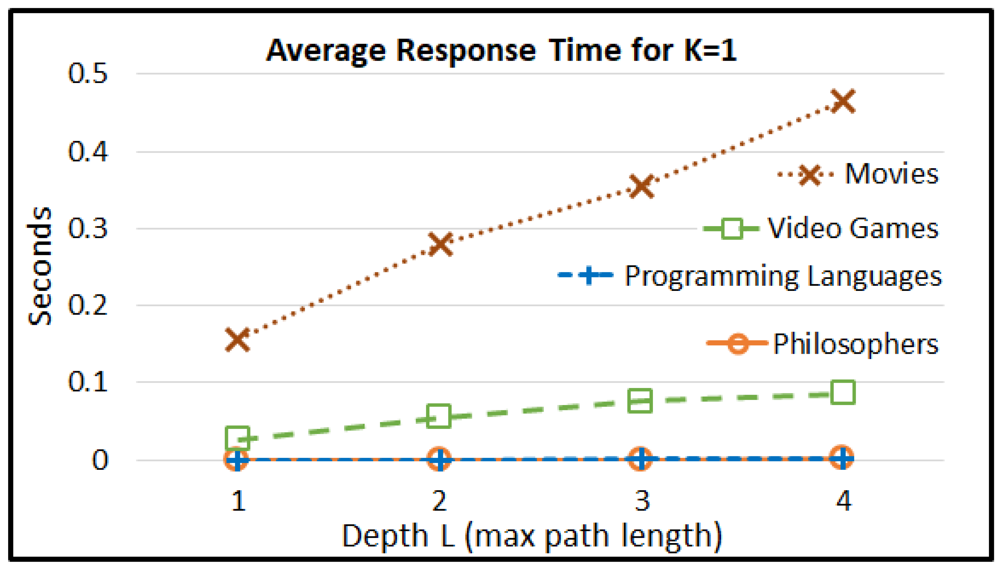
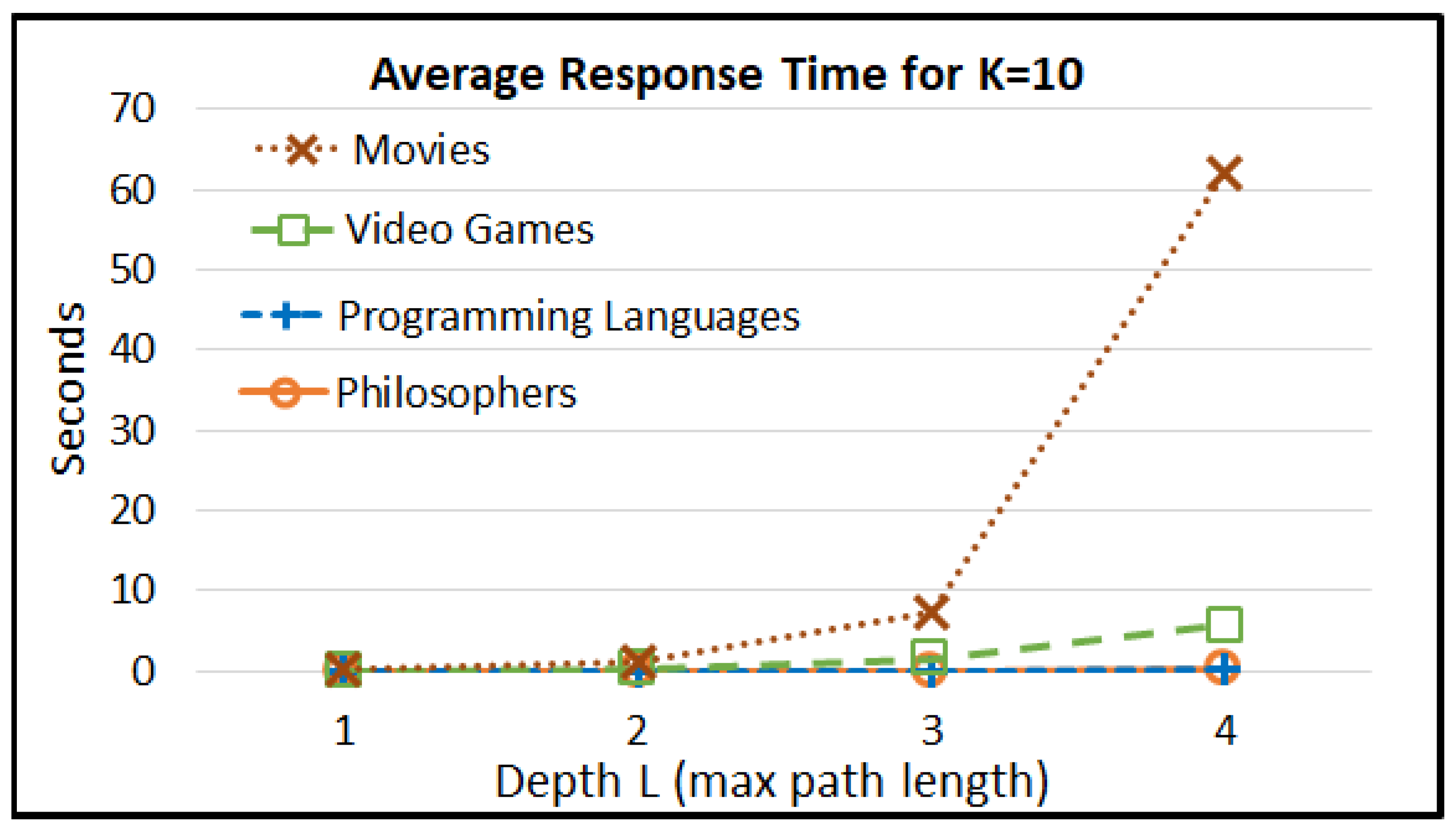
5.2.2. Efficiency Measurements

Here, we provide some measurements about the efficiency of RDFsim. We provide results for the execution time (i) for creating the embeddings and the indexes, (ii) for retrieving the desired data for the default case, that is, for browsing the top-10 similar entities to an entity, and (iii) cases when larger similarity graphs are created.

Measurements for the Creation of Embeddings and Indexes. Here, we measure the execution time for creating the embeddings and the indexes. Based on the literature for RDF knowledge graph embeddings [10,32], we selected the following parameters for the skip-gram model of word2vec: minwordFrequency = 5, that is, the minimum number of times a URI must appear in the corpus (e.g., in our case if a URI appears less than five times, it is not learned), window size = 3, that is, the context window, iter = 10, that is, number of iterations over the text corpus, and layersize = 200, that is, the number of dimensions of each vector.

Table 3. Execution Time (in seconds) for creating the embeddings and the indexes.

DBpedia Dataset	Embeddings Creation Time	Indexing Creation Time	Total Time
Philosophers	5.8 s	5.3 s	11.1 s
Programming Languages	11.1 s	16.6 s	27.1 s
Video Games	535.8 s	1408.4 s	1944.2 s
Movies	2338.3 s	27,716.6 s	30,054.9 s
Total	2891.0 s	29,146.9 s	32,037.3 s

introduces the results for each dataset, that is, for creating the embeddings we needed from 5.8 s to 38.9 m, whereas for the indexes, 5.3 s to 7.6 h. For both tasks, we needed from 11.1 s to 8 h. In total, 8.9 h were needed for all the datasets to complete all the tasks. Although this process can be time-consuming for large datasets (e.g., 32 min for Video Games and 8 h for Movies), it is performed only once, that is, for offering similarity-based browsing, we just need the produced indexes of this process.

Measurements for the Default Similarity Graph.

Table 4. Average execution time (in seconds) for retrieving the desired data for an entity and for creating its default similarity graph.

DBpedia Dataset	Browse Entity-Sequential Access	Browse Entity-Random Access	Speedup from Random Access
Philosophers	0.00502 s	0.00044 s	11.40×
Programming Languages	0.01756 s	0.00132 s	13.30×
Video Games	0.37720 s	0.02257 s	16.71×
Movies	1.98209 s	0.13247 s	14.96×

presents the results for the average response time of retrieving the desired data for an entity from Entity Index and for creating the default graph containing its top-10 similar entities. As we can see, as the size of a dataset grows, the execution time increases. However, by using the Pointers Index the average time is quite low even for larger datasets, for example, for Movies (i.e., the largest dataset) RDFsim needs on average 0.13 s to show to the user the resulting page for an entity. Finally, the gain of using a random access (through Pointers Index) instead of a sequential access is obvious, that is, the speedup varies from 11.4× to 16.71× for the four different DBpedia datasets.

Measurements for Similarity Graphs Containing Larger Paths. Here, we measure the time for creating larger similarity graphs for different values of K and L, for each of the four DBpedia datasets. For performing these measurements, we randomly selected ten entities from each dataset, and we computed the average time to create the desired similarity graph. We present one figure for each different value of K, that is, Figure 9 for $K=1$, Figure 10 for $K=5$, Figure 11 for $K=10$ and Figure 12 for $K=15$.

Concerning the results, for a small value of K, that is, $K=1$ or $K=5$ (i.e., Figure 9 and Figure 10), the similarity graph is created quite fast when $L\le 4$. However, due to the exponential nature of the algorithm concerning the number of nodes and edges (see Section 4.3), the execution time can be very high as the depth L increases, especially for large values of K and large datasets. For example, for the dataset of Movies the execution time highly increases when L and K grows (i.e., when larger paths are created), for example, for $K=10$ and $L=4$ the execution time was 62 s (see Figure 11), whereas the corresponding time for $K=15$ and $L=4$ was 149 s (see Figure 12).

5.2.3. Indicative Measurements for the Results of the Embeddings

Here, we provide some indicative measurements for evaluating the results of the embeddings. Since the evaluation of embeddings process requires a further analysis (which is one of our future targets), that is, to compare the results by using different parameters and specialized evaluation collections; here, we introduce some indicative results for two specific entities, that is, for the entities “Aristotle” and “Python Programming Language” from the datasets of “Philosophers” and “Programming Languages”, respectively.

What we measure. We measure the number of entities in the top-K similar entities of each entity that are not directly connected and the common values among two entities.

Similar but not Neighbors. Remember that for a single entity e, we denote as $similars(e,K)$ the entities belonging to its top-K. Moreover, as $similars{(e,K)}_{Conn}$ we denote the set of entities belonging to the top-K similar entities of e and there is a direct connection between e and each of them (through a triple), that is, $similars{(E,K)}_{Conn}=\{e^{\prime }\in similars(e,K)|\langle e,p,e^{\prime }\rangle \in Tor\langle e^{\prime },p,e\rangle \in T\}$, where T is the set of triples. On the contrary, we denote as $similars{(e,K)}_{noConn}$, the similar entities that are not connected with a triple, that is, $similars{(e,K)}_{noConn}=similars(e,K)\backslash similars{(e,K)}_{Conn}$.

For computing these sets, we send the following SPARQL queries between the focused entity e and each of the entities $e^{\prime }\in similars(e,K)$: “ASK WHERE {e ?p $e^{\prime }$}” and “ASK WHERE {$e^{\prime }$ ?p e}”. If both queries return false, it means that these two entities are not connected through a triple (i.e., $e^{\prime }\in similars{(e,K)}_{noConn}$).

Common Values. For each pair containing entity e and each $e^{\prime }\in similars(e,K)$, we measure the number of common subject-predicate pairs, where $commonSP(e,e^{\prime })=\left\{\{p,o\}\right|\langle e,p,o\rangle \in Tand\langle e^{\prime },p,o\rangle \in T\}$ and predicate-object pairs, where $commonPO(e,e^{\prime })=\left\{\{s,p\}\right|\langle s,p,e\rangle \in Tand\langle s,p,e^{\prime }\rangle \in T\}$. For computing $commonSP(e,e^{\prime })$ we send the SPARQL query “Select count(*) WHERE {$e^{\prime }$ ?p ?o. e ?p ?o}” whereas the corresponding SPARQL query for $commonPO(e,e^{\prime })$ is the following: “Select count(*) WHERE { ?s ?p $e^{\prime }$ . ?s ?p e}”. In the end, we sum the cardinality of these two results for finding the number of common values between these two entities, that is, $|commonValues(e,e^{\prime })|=|commonSP(e,e^{\prime })|+|commonPO(e,e^{\prime })|$.

Indicative Results.

Table 5. Similarity Measurements for the top-10 similar entities to Aristotle.

Position	Entity ${\mathit{e}}^{\prime }$	Sim. Score	${\mathit{e}}^{\prime }$ Belongs to $\mathit{Similars}{(\mathit{e},\mathit{K})}_{\mathit{Conn}}$	$\left|\mathit{commonValues}\right(\mathit{e},{\mathit{e}}^{\prime }\left)\right|$
1	Plato	0.53	✓	3084
2	Socrates	0.51	✓	984
3	Ancient Greek philosophy	0.47	✓	586
4	Cicero	0.46	✓	810
5	Platonism	0.46	✓	304
6	Arcesilaus	0.45		50
7	Diogenes Laertius	0.45		173
8	Athens	0.43	√	710
9	Zeno of Citium	0.42		158
10	Universal (metaphysics)	0.42		114

shows the results for Aristotle, whereas

Table 6. Similarity Measurements for the top-10 similar entities to Python Programming Language.

Position	Entity ${\mathit{e}}^{\prime }$	Sim. Score	${\mathit{e}}^{\prime }$ Belongs to $\mathit{Similars}{(\mathit{e},\mathit{K})}_{\mathit{Conn}}$	$\left|\mathit{commonValues}\right(\mathit{e},{\mathit{e}}^{\prime }\left)\right|$
1	Java	0.59	✓	2386
2	Ruby	0.57	✓	1450
3	Compiler	0.56	✓	478
4	Open-source software	0.55		1048
5	Object-oriented programming	0.55	✓	502
6	C++	0.54	✓	1508
7	C Sharp	0.54	√	1270
8	Graphical user interface	0.53	✓	602
9	Reflective programming	0.53	✓	124
10	BASIC	0.50		260

for “Python programming language”, respectively. As we can see, in both cases most of their similar entities are also their direct neighbours, that is, six out of ten cases for “Aristotle” and eight out of ten cases for “Python”. On the contrary, there are entities belonging to their top-10 similar entities, and there is not a direct connection between them and the desired entity, for example, “Diogenes Laertius”, “Open source software”, and so forth. However, these entities share several common values with the desired entities, for example, “Diogenes Laertius” share 173 common values with “Aristotle” and “Open-source software” share 1048 common values with “Python programming language”.

6. Use Cases

Here, we describe three use cases of RDFsim similarity browsing, by using real examples (taken from RDFsim), for illustrating the functionality of RDFsim.

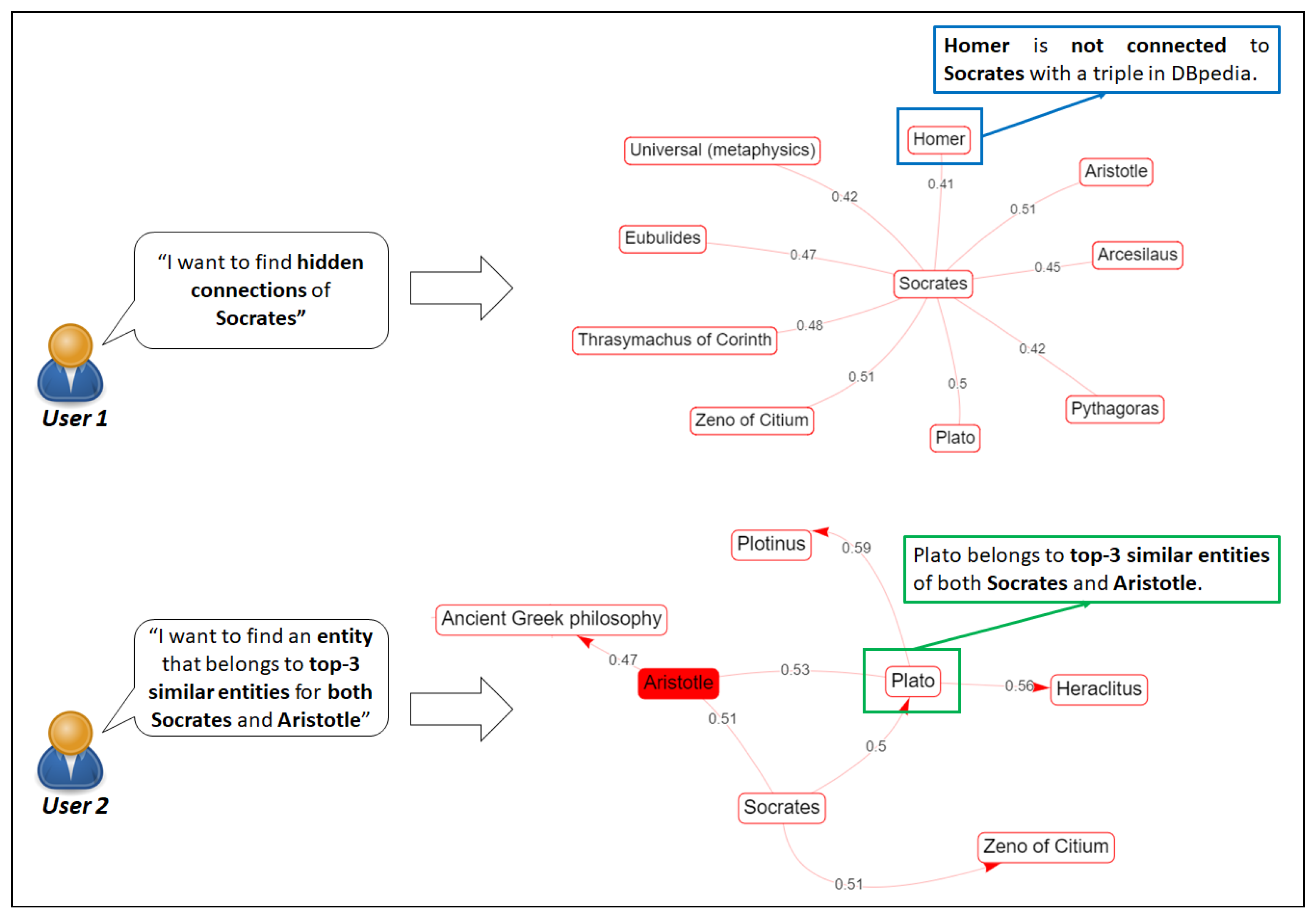
6.1. Use Case 1. “Parallel Browsing” of the Entity in Focus

Suppose that a user desires to browse the triples of an entity, to see its corresponding DBpedia or Wikidata page and to find its similar entities. This can be feasible by connecting to several web applications, for example, by browsing its corresponding DBpedia and Wikidata pages, and also by using a system such as KGvec2go [11] or Wembedder [33] for finding its similar entities. However, the above process should be done separately for each different entity and it is not feasible to access that information in a single page. On the contrary, through RDFsim this functionality is offered in parallel, that is, in a single page, by using two different frames, for example, see Figure 5. Moreover, by interacting with any of the two frames of RDFsim, that is, by clicking to any entity, the page is automatically refreshed for showing the desired information for that entity.

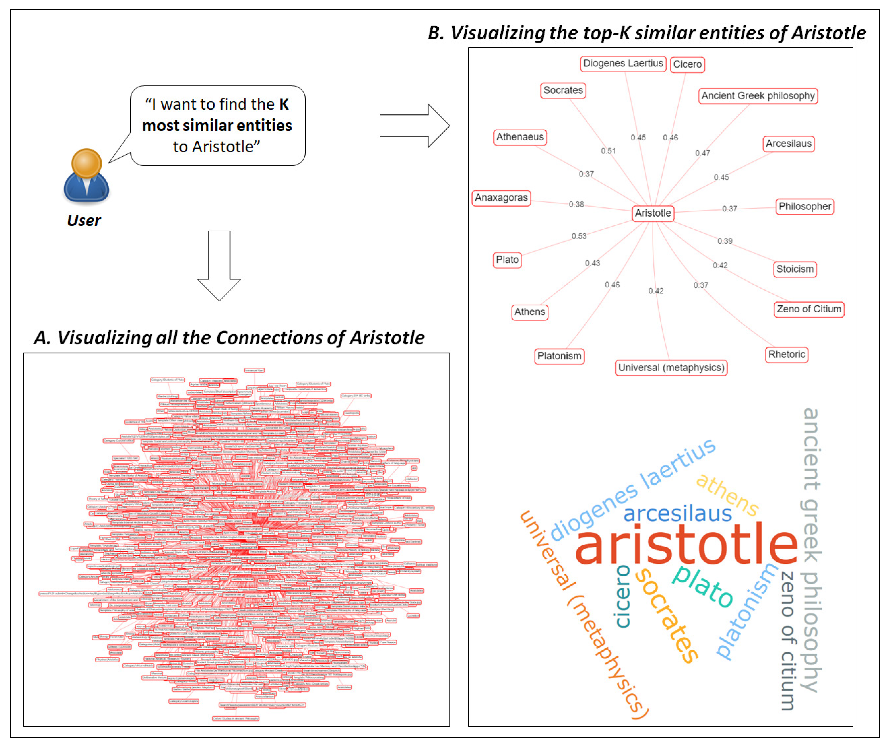
6.2. Use Case 2. Finding the Most Similar Entities of a Popular Entity

Suppose a scenario that a user desires to find the top-K similar entities to “Aristotle”. By using any of the browsing systems presented in Section 5.1, one way is to check the entities that are connected to “Aristotle”, for indicating which of them are similar. However, this task can be quite difficult and expensive for many entities. Indicatively, “Aristotle” in DBpedia KB is directly connected with over 1000 entities, as it is also depicted in the left side of Figure 13. Through such a visualization, it is extremely difficult to identify similar entities. On the contrary, through RDFsim it is feasible to restrict the results, since it visualizes the top-K entities of each entity very fast, through different visualizations, for example, see the right side of Figure 13.

6.3. Use Case 3. Discovering “Hidden” Similarity-Based Connections between Entities

Except for the direct connections, as we have seen in Section 5.2.3, there are entities that are discovered similar through RDFsim and there is not a direct connection between them (i.e., see Table 5 and Table 6). For instance, suppose that a user desires to find such “hidden” connections for the entity “Socrates”, that is, see the first user in the left upper side of Figure 14. In this paradigm (taken from RDFsim), we found that the poet “Homer” belongs to the top-K similar entities of the philosopher “Socrates”, but these entities are not connected through a triple in DBpedia. Thereby, by browsing only the direct triples either of “Socrates” or of “Homer”, it would be infeasible to discover such a similarity. On the contrary, through RDFsim such similarities can be browsed. For the given example, these two entities share 348 common values, that is, predicate-object and subject-object pairs in DBpedia Knowledge base, therefore it seems rational that these entities computed as similar from the embeddings model.

In another scenario, that is, see the second user in Figure 14, suppose that one desires to conduct a further analysis, that is, to find the intersection of top-3 similar entities between two entities, say “Aristotle” and “Socrates”. Since RDFsim offers visualizations of large paths, it is feasible as it is shown in Figure 14, that is, we can observe that the entity “Plato” belongs to the top-3 similar entities for both “Aristotle” and “Socrates”.

7. Concluding Remarks

Since browsing is the core access method for the Web from its beginning, it is worth investigating browsing methods that are appropriate for the Web of Data, that is, capable to distinguish the most important connections and reveal hidden relationships. Towards this general direction, in this paper we presented RDFsim, a similarity-based browsing system for RDF datasets. The novelty of RDFsim comparing to existing browsing systems, is that it offers “Parallel Browsing” by enabling user to browse not only the original data (i.e., triples) of a selected entity, but also its K most similar entities (even if they are not directly connected) in the form of an interactive graph or a tagCloud visualization. The similarity of entities is founded on word (in our case URI) embeddings (computed through word2vec skip-gram model), however we introduced indexes for enabling real-time interaction, which do not depend on the particular method for computing similarity. Currently, RDFsim provides the aforementioned functionality for 345 thousand entities from 4 subsets of DBpedia (containing movies, philosophers, video games and programming languages).

We showed that with the produced indexes, one can browse very fast the similar entities of a given entity (e.g., for a given movie on average 0.13 seconds are needed), and can discover “hidden” similarity-based connections among entities, that is, entities that are similar but there is no direct connection between them in the dataset. As regards use cases, we introduced scenarios showcasing the flexibility of RDFsim for browsing all the information of each entity and its top-K similar entities at the same time, and for discovering “hidden” relationships by following similarity paths.

As a future work, we plan to support more RDF datasets (apart from DBpedia) and to enhance the scalability of the indexing process, since the computation of the embeddings and the construction of the indexes can be time-consuming if the number of triples is very big (e.g., more than 8 h are needed for DBpedia Movies dataset with 13 million triples). Consequently, for supporting similarity-based browsing over big knowledge graphs, comprising billions of triples, it is worth investigating methods for parallelizing the indexing process. Furthermore, we plan to evaluate the effectiveness of the embebbings, by comparing different parameters and embedding models (such as BERT [37], GloVE [38] and FastText [39]). For achieving this target, we plan to extend RDFsim for supporting precomputed similarity results, produced through any similarity method [29], and to use specialized evaluation collections, using a task-based evaluation with users, for getting feedback also for the interaction. Another topic that is worth further research is to test embeddings construction methods that also exploit the literals of RDF datasets (such methods are surveyed in [35]). Finally, as regards visualization, it is worth investigating alternative methods that can show more values in less space while making clear their importance and context.

References

1. Nikas, C.; Kadilierakis, G.; Fafalios, P.; Tzitzikas, Y. Keyword Search over RDF: Is a Single Perspective Enough? Big Data Cogn. Comput. 2020, 4, 22. [Google Scholar] [CrossRef]
2. Ilievski, F.; Beek, W.; van Erp, M.; Rietveld, L.; Schlobach, S. LOTUS: Adaptive text search for big linked data. In Proceedings of the European Semantic Web Conference, Kobe, Japan, 17–21 October 2016; Springer: Berlin/Heidelberg, Germany, 2016; pp. 470–485. [Google Scholar]
3. Camarda, D.V.; Mazzini, S.; Antonuccio, A. LodLive, exploring the web of data. In Proceedings of the 8th International Conference on Semantic Systems, Graz, Austria, 5–7 September 2012; pp. 197–200. [Google Scholar]
4. Micsik, A.; Turbucz, S.; Györök, A. Lodmilla: A linked data browser for all. Information 2014, 31–34. [Google Scholar]
5. Atzori, M.; Mazzeo, G.M.; Zaniolo, C. QA3: A natural language approach to question answering over RDF data cubes. Semant. Web 2019, 10, 587–604. [Google Scholar] [CrossRef]
6. Arenas, M.; Grau, B.C.; Kharlamov, E.; Marciuška, Š.; Zheleznyakov, D. Faceted search over RDF-based knowledge graphs. J. Web Semant. 2016, 37, 55–74. [Google Scholar] [CrossRef]
7. Tzitzikas, Y.; Manolis, N.; Papadakos, P. Faceted exploration of RDF/S datasets: A survey. J. Intell. Inf. Syst. 2017, 48, 329–364. [Google Scholar] [CrossRef]
8. Kritsotakis, V.; Roussakis, Y.; Patkos, T.; Theodoridou, M. Assistive Query Building for Semantic Data. In Proceedings of the SEMANTICS Posters & Demos, Vienna, Austria, 10–13 September 2018. [Google Scholar]
9. Lehmann, J.; Isele, R.; Jakob, M.; Jentzsch, A.; Kontokostas, D.; Mendes, P.N.; Hellmann, S.; Morsey, M.; Van Kleef, P.; Auer, S.; et al. Dbpedia—A large-scale, multilingual knowledge base extracted from wikipedia. Semant. Web 2015, 6, 167–195. [Google Scholar] [CrossRef] [Green Version]
10. Ristoski, P.; Rosati, J.; Di Noia, T.; De Leone, R.; Paulheim, H. RDF2Vec: RDF graph embeddings and their applications. Semant. Web 2019, 10, 721–752. [Google Scholar] [CrossRef] [Green Version]
11. Portisch, J.; Hladik, M.; Paulheim, H. KGvec2go–Knowledge Graph Embeddings as a Service. arXiv 2020, arXiv:2003.05809. [Google Scholar]
12. Mountantonakis, M.; Tzitzikas, Y. Knowledge Graph Embeddings over Hundreds of Linked Datasets. In Proceedings of the Research Conference on Metadata and Semantics Research, Rome, Italy, 28–31 October 2019; Springer: Berlin/Heidelberg, Germany, 2019; pp. 150–162. [Google Scholar]
13. Moreno-Vega, J.; Hogan, A. GraFa: Scalable faceted browsing for RDF graphs. In Proceedings of the International Semantic Web Conference, Monterey, CA, USA, 8–12 October 2018; Springer: Berlin/Heidelberg, Germany, 2018; pp. 301–317. [Google Scholar]
14. Mikolov, T.; Chen, K.; Corrado, G.; Dean, J. Efficient estimation of word representations in vector space. arXiv 2013, arXiv:1301.3781. [Google Scholar]
15. Mikolov, T.; Sutskever, I.; Chen, K.; Corrado, G.; Dean, J. Distributed representations of words and phrases and their compositionality. arXiv 2013, arXiv:1310.4546. [Google Scholar]
16. Wylot, M.; Hauswirth, M.; Cudré-Mauroux, P.; Sakr, S. RDF data storage and query processing schemes: A survey. ACM Comput. Surv. (CSUR) 2018, 51, 1–36. [Google Scholar] [CrossRef]
17. Elbassuoni, S.; Blanco, R. Keyword search over RDF graphs. In Proceedings of the 20th ACM International Conference on Information and Knowledge Management, Scotland, UK, 24–28 October 2011; pp. 237–242. [Google Scholar]
18. Delbru, R.; Rakhmawati, N.A.; Tummarello, G. Sindice at semsearch 2010. In Proceedings of the 19th International World Wide Web Conference, Raleigh, NC, USA, 26–30 April 2010. [Google Scholar]
19. Liu, X.; Fang, H. A study of entity search in semantic search workshop. In Proceedings of the 3rd International Semantic Search Workshop, Raleigh, NC, USA, 26 April 2010. [Google Scholar]
20. Kadilierakis, G.; Nikas, C.; Fafalios, P.; Papadakos, P.; Tzitzikas, Y. Elas4RDF: Multi-perspective triple-centered keyword search over RDF using elasticsearch. In Proceedings of the European Semantic Web Conference, Virtual online, 1–6 November 2020; Springer: Berlin/Heidelberg, Germany, 2020; pp. 122–128. [Google Scholar]
21. Vega-Gorgojo, G.; Slaughter, L.; Von Zernichow, B.M.; Nikolov, N.; Roman, D. Linked data exploration with RDF surveyor. IEEE Access 2019, 7, 172199–172213. [Google Scholar] [CrossRef]
22. Papadaki, M.E.; Spyratos, N.; Tzitzikas, Y. Towards Interactive Analytics over RDF Graphs. Algorithms 2021, 14, 34. [Google Scholar] [CrossRef]
23. Colazzo, D.; Goasdoué, F.; Manolescu, I.; Roatiş, A. RDF analytics: Lenses over semantic graphs. In Proceedings of the 23rd International Conference on World Wide Web, Seoul, Korea, 7–11 April 2014; pp. 467–478. [Google Scholar]
24. Zou, L.; Huang, R.; Wang, H.; Yu, J.X.; He, W.; Zhao, D. Natural language question answering over RDF: A graph data driven approach. In Proceedings of the 2014 ACM SIGMOD International Conference on Management of Data, Snowbird, UT, USA, 22–27 June 2014; pp. 313–324. [Google Scholar]
25. Bast, H.; Haussmann, E. More accurate question answering on freebase. In Proceedings of the 24th ACM International on Conference on Information and Knowledge Management, Melbourne, VIC, Australia, 19–23 October 2015; pp. 1431–1440. [Google Scholar]
26. Shekarpour, S.; Marx, E.; Ngomo, A.C.N.; Auer, S. Sina: Semantic interpretation of user queries for question answering on interlinked data. J. Web Semant. 2015, 30, 39–51. [Google Scholar] [CrossRef]
27. Dimitrakis, E.; Sgontzos, K.; Tzitzikas, Y. A survey on question answering systems over linked data and documents. J. Intell. Inf. Syst. 2019, 55, 1–27. [Google Scholar] [CrossRef]
28. Nikas, C.; Fafalios, P.; Tzitzikas, Y. Open Domain Question Answering over Knowledge Graphs using Keyword Search, Answer Type Prediction, SPARQL and Pre-trained Neural Models. In Proceedings of the 20th International Semantic Web Conference, Virtual online, 24–28 October 2021; Springer: Berlin/Heidelberg, Germany, 2021. [Google Scholar]
29. Chandrasekaran, D.; Mago, V. Evolution of Semantic Similarity—A Survey. ACM Comput. Surv. (CSUR) 2021, 54, 1–37. [Google Scholar] [CrossRef]
30. Albertoni, R.; De Martino, M. Asymmetric and context-dependent semantic similarity among ontology instances. In Journal on Data Semantics X; Springer: Berlin/Heidelberg, Germany, 2008; pp. 1–30. [Google Scholar]
31. Hickson, M.; Kargakis, Y.; Tzitzikas, Y. Similarity-based browsing over linked open data. arXiv 2011, arXiv:1106.4176. [Google Scholar]
32. Mountantonakis, M.; Tzitzikas, Y. Applying cross-data set identity reasoning for producing URI embeddings over hundreds of RDF data sets. Int. J. Metadata Semant. Ontol. 2021, 15, 1–22. [Google Scholar] [CrossRef]
33. Nielsen, F.Å. Wembedder: Wikidata entity embedding web service. arXiv 2017, arXiv:1710.04099. [Google Scholar]
34. Mountantonakis, M.; Tzitzikas, Y. Content-based union and complement metrics for dataset search over RDF knowledge graphs. J. Data Inf. Qual. (JDIQ) 2020, 12, 1–31. [Google Scholar] [CrossRef]
35. Gesese, G.A.; Biswas, R.; Alam, M.; Sack, H. A survey on knowledge graph embeddings with literals: Which model links better literal-ly? Semant. Web 2019, 12, 617–647. [Google Scholar] [CrossRef]
36. Kastrinakis, D.; Tzitzikas, Y. Advancing search query autocompletion services with more and better suggestions. In Proceedings of the International Conference on Web Engineering, Vienna, Austria, 5–9 July 2010; Springer: Berlin/Heidelberg, Germany, 2010; pp. 35–49. [Google Scholar]
37. Devlin, J.; Chang, M.W.; Lee, K.; Toutanova, K. Bert: Pre-training of deep bidirectional transformers for language understanding. arXiv 2018, arXiv:1810.04805. [Google Scholar]
38. Pennington, J.; Socher, R.; Manning, C.D. Glove: Global vectors for word representation. In Proceedings of the 2014 Conference on Empirical Methods in Natural Language Processing (EMNLP), Doha, Qatar, 25–29 October 2014; pp. 1532–1543. [Google Scholar]
39. Bojanowski, P.; Grave, E.; Joulin, A.; Mikolov, T. Enriching word vectors with subword information. Trans. Assoc. Comput. Linguist. 2017, 5, 135–146. [Google Scholar] [CrossRef] [Green Version]
40. Tzitzikas, Y.; Papadaki, M.; Chatzakis, M. A Spiral-like Method to Place in the Space (and Interact with) too Many Values. J. Intell. Inf. Syst. 2021, in press. [Google Scholar]
41. Vrandečić, D.; Krötzsch, M. Wikidata: A free collaborative knowledgebase. Commun. ACM 2014, 57, 78–85. [Google Scholar] [CrossRef]
Figure 1. An Overview of Access Methods over RDF.
Information 12 00440 g001
Figure 2. The default browsing system of RDFsim for the entity “Socrates”.
Information 12 00440 g002
Figure 3. The two processes of RDFsim.
Information 12 00440 g003
Figure 4. The process of Finding and Storing the Top-K similar entities through embeddings in specialized indexes.
Information 12 00440 g004
Figure 5. Parallel Browsing for the selected entity Aristotle.
Information 12 00440 g005
Figure 6. Constructing the Similarity Graph for “Socrates” with parameters K = 2 and L = 2 .
Information 12 00440 g006
Figure 7. The resulting Similarity Graph for “Toy Story” Movie with parameters K = 3 and L = 3 .
Information 12 00440 g007
Figure 8. TagCloud visualization for the 10 most similar entities to the entity “History”.
Information 12 00440 g008
Figure 9. Average time for creating the similarity graph for K = 1 .
Information 12 00440 g009
Figure 10. Average time for creating the similarity graph for K = 5 .
Information 12 00440 g010
Figure 11. Average time for creating the similarity graph for K = 10 .
Information 12 00440 g011
Figure 12. Average time for creating the similarity graph for K = 15 .
Information 12 00440 g012
Figure 13. Discovering Similar Entities for the selected entity “Aristotle”.
Information 12 00440 g013
Figure 14. Discovering “Hidden” Similarity-Based Connections between Entities.
Information 12 00440 g014